Stochastic Logic Programs: Sampling, Inference and Applications

James Cussens

Department of Computer Science, University of York

Heslington, York, Y OlO SDD, U K jc®cs.york. ac.uk

Abstract

Algorithms for exact and approximate inference in stochastic logic programs ( SLPs) are pre­ sented, based respectively, on variable elimina­ tion and importance sampling. We then show how SLPs can be used to represent prior distri­ butions for machine learning, using (i) logic pro­ grams and (ii) Bayes net structures as examples. Drawing on existing work in statistics, we apply the Metropolis- Hasting algorithm to construct a Markov chain which samples from the posterior distribution. A Prolog implementation for this is described. We also discuss the possibility of con­ structing explicit representations of the posterior.

1 Introduction

A stochastic logic program ( SLP) is a probabilistic exten­ sion of a normal logic program that has been proposed as a flexible way of representing complex probabilistic knowl­ edge; generalising, for example, Hidden Markov Models, Stochastic Context- Free Grammars and Markov nets ( Mug­ gleton, 1996; Cussens, 1999). However, we need to ask (i) whether this increase in flexibility is needed for any real problems and (ii) whether reasonable algorithms exist for inference and learning in SLPs.

In this paper we give a number of approaches to approx­ imate and exact inference in SLPs, focusing mostly on sampling. More importantly, we apply SLPs to an impor­ tant problem-Bayesian machine learning-which would be difficult to handle with simpler representations.

The paper is organised as follows. Section 2 contains essential de finitions from logic programming. Section 3 shows we can use SLPs to define three different sorts of distributions, but focuses on the appealingly simple loglin­ ear model. Sections 4 and 5 give two quite different ways of improving sampling for the loglinear model, being based on Pro log and importance sampling, respectively. Section 6

briefly shows how variable elimination can be used for ex­ act inference in SLPs. After showing how to extend SLPs with non-equational constraints in Section 7, we can finally bring much of the preceding work together in Sections 8 and 9 to show how SLPs can be used to represent distribu­ tions over complex model spaces, such as is required for 'really Bayesian' machine learning. Section 10 contains conclusions and pointers to possible future work.

2 Logic Programming Essentials

An overview of logic programming can be found in (Cussens, 1999). Here, lack of space means that only the most important definitions are flagged. An SLD-derivation of a goal G0 using a logic program P is a (finite or infi­ nite) sequence { Statej} j, each element of which is either a 4-tuple ( G i, Aj, Cj, () i) or the empty goal D where

• Ai is the selected atom of goal Gi;
• Cj is the selected input clause in P, with its variables renamed so that Ci and G i have no variables in com­ mon;
• Bi is the most general unifier of Ai and Cj (the head of cj) or fail if they can not be unified.
• If ()i = fail then Statej+1 = fail. Otherwise, Gi+1 is the result of replacing Ai by Cj (the body of Cj) in Gj and then applying ()i to the result. If Gi+1 = D then Statej+l = D.

An SLD-refutation is a finite SLD-derivation ending in the empty goal D. The SLD-tree for a goal G is a tree of goals, with G as root node, and such that the children of any goal G' are goals produced by one resolution step using G' (D and fail have no children). Fig 6 shows an SLD-tree. A computed answer for a goal is a substitution for the vari­ ables in G produced by an SLD-refutation of G.

3 Defining Distributions with SLPs

A stochastic logic program ( SLP) is a logic program where some of the predicates (the distribution-defining or proba­ bilistic predicates) have non-negative numbers attached to the clauses which make up their definitions. We denote the label for a Clause Ci by li. We also write Ai = lo g l i , and we denote the parameter vector containing all the Ai by A. In this paper we will consider only normalised SLPs where labels for the clauses making up the definition of a predi­ cate sum to one.

The basic idea is that clause labels probabilistically influ­ ence which input clause is chosen as a derivation proceeds, thus de fining a distribution over derivations from which distributions over (i) refutations and (ii) variable bindings may be derived. We begin by restricting attention to pure SLPs, where all predicates have labelled de finitions, post­ poning the impure case until Section 7.

3.1 Loglinear Model

Given an SLP S with parameters A and a goal Go we can sample SLD-derivations for Go using loglinear sampling as follows:

Loglinear sampling: Any computation rule may be used to select the atom Aj from the current goal G i. The next input clause Cj is chosen with probability li from those clauses in S with the same predicate symbol in the head as Aj. We stop when we produce either fail or D.

Let R( G) denote the set of refutations of the goal G (i. e. derivations that end in D). Let vi (r) be the number of times labelled clause Ci is used in refutation r. The loglinear distribution P(>.,S,G) over refutations r of the goal G is

where

The loglinear distribution over all derivations, which in­ cludes in finite ones and ones ending in fail, is similar except that Z(>.,S,G) is guaranteed to equal one.

Computing the unnormalised probability (potential) 'ljJ of an already given refutation is efficient, since we just multi­ ply clause labels as we go. Loglinear sampling to produce a refutation is less efficient. It is essentially the same as for­ ward sampling in Bayesian networks and suffers from the same defect: inefficiency when sampling from a distribu­ tion conditional on evidence. In the case of SLPs the same problem arises when, as is usually the case, we are only in­ terested in refutations-which are derivations conditional on their last goal being the empty goal. Sampling from the full set of derivations, including failed ones, is easy.

The problem is the restricted information that is readily available when selecting the next input clause. Let us call z (>.,S,G) the weight of the SLD-tree under G or briefly the weight of G. If we had the weights of the potential suc­ cessor goals each possible input clause would give, then we could sample easily from the loglinear model by sim­ ply making choices in proportion to these weights. The stochastic search rule thus implemented would never fol­ low a failure branch, since such branches have zero weight.

If IR(G)I is reasonably small then we can simply use Pro­ log to find all r E R( G) together with their probabilities P(>.,S,G)(r), store this information in a simple table and then sample the r E R(G) according to P(>.,s,a )(r) . In some applications the central problem is searching a pos­ sibly very large SLD-tree for a few refutations-for this we can use normal logic programming approaches. In par­ ticular, chart-based and/or bottom-up approaches to finding refutations will often be appropriate. In statistical computa­ tional linguistics, refutations amount to parses, and there is a substantial body of work on finding parses and their prob­ abilities. Usually interest is confined to finding the single most likely parse. For example, ( Riezler, 1998) presents an approach to this problem that trades ef ficiency for optimal­ ity in a generalisation of the Viterbi algorithm using Earley deduction. ( Muggleton, 2000) presents an algorithm that enumerates refutations in order of decreasing probability. ( Muggleton, 2000) also discusses how to unfold an SLP to make it 'more tabular' .

However, many interesting applications will involve goals with large, even infinitely many refutations. In such cases, both loglinear sampling and "all refutations sampling" can both be very inefficient. In the next two sections, we con­ sider altern atives which lead to more efficient sampling.

3.2 Unification-constrained Model

Unification-constrained sampling finds refutations more efficiently than loglinear sampling because it only chooses clauses from amongst those that unify with the selected atom. It effects a one-step lookahead by examining po­ tential input clauses before selecting one. Let unif(Aj) be the set of clauses whose heads unify with the atom Ai.

Unification-constrained sampling: The selected atom Ai is always the leftmost atom in the cur­ rent goal G i. The next input clause Cj is chosen from unif(Aj) with probability proportional to l j . We stop when we produce either fail or D.

This is the original sampling mechanism defined by ( Mug­ gleton, 1996). It is a theorem of logic programming that normal SLD-refutation is essentially unaltered by chang­ ing the atom selection rule (although drastic changes in ef­ ficiency can occur). If we delay selecting an atom A, all that changes is that A may be more instantiated when we eventually do select it. Unfortunately, this means that de­ laying the selection of A will alter unif(A) and so we are obliged to fix the selection rule in unification-constrained sampling so that a single distribution is de fined.

The uni fication-constrained distribution P( .x,s ,G) over refu­ tations for a goal G is

where

Computing the unnormalised probability (potential) '1/! u of a refutation is only slightly less easy than with the loglinear model, since all the values li'· for Ci' E unif(Aj), can be quickly found as the refutation proceeds.

3.3 Backtrackable Model

Uni fication-constrained sampling stops as soon as it reaches fail, backtrackable sampling backtracks upon failure, and so will generally be a more efficient way of sampling refutations. Backtrackable sampling is essen­ tially Pro log with a probabilistic clause selector.

Backtrackable sampling: The selected atom Ai is always the leftmost atom in the current goal G i . The next input clause Cj is chosen with probability li. If we produce fail then we backtrack to the most recent choice-point, delete the choice of input clause that led to failure and choose from amongst the surviving choices with probability proportional to clause labels. If no choices remain then we backtrack further until a choice can be made or return fail. We stop if we produceD or fail.

Let succ(Aj) be the set of input clauses which lead to at least one refutation. The backtrackable distribution Pt.x , S,G) over refutations for a goal G is

where

Computing the unnormalised probability (potential) '1/Jb of a refutation is, in general, hard; since we may have to ex­ plore a very large SLD-tree rooted at G i to identify the set succ(Aj).

Comparing the loglinear, uni fication-constrained and back­ trackable models we see there is a trade-off between ease of sampling a refutation, and ease of computing a potential for a given refutation. If only sampling is required and we are happy that the order of literals in clauses matters, then the backtrackable model makes sense. However, the loglin­ ear model has attractively simple mathematical properties which we will exploit in the MC MC application. Fortu­ nately, loglinear sampling can be sped up as the next sec­ tion shows.

4 Improving Loglinear Sampling

( Muggleton, 1996) explicitly introduced SLPs as general­ isations of Hidden Markov models (H M Ms) and Stochas­ tic Context- Free Grammars ( SC FGs). Comparing SLPs to H M Ms we see that in SLPs: (i) the states of an H M M are replaced by goals (ii) the outputs of an H M M are replaced by substitutions (iii) concatenation of outputs is replaced by composition of substitutions (iv) outputs (substitutions) are generated deterministically and (v) state transition proba­ bilities are given by clause labels. It is also more natural in SLPs to associate outputs (substitutions) with transitions between states (goals) rather than with states themselves.

The connection between SLPs and SC FGs is even closer. Consider S1, the SC FG in Fig 1 which has been imple­ mented as an SLP. We can generate sentences using log­ linear sampling with the goal : -s (A, [] ) . Since S1 is an SC FG, the query will always succeed, even though we do not allow backtracking in the loglinear model. Suppose

Figure 1: S1: An SC FG

now, that we are interested only in reflexive sentences. We then apply a constraint to the SC FG: replacing l:s(A,B) n(A,C), v(C,D), n(D,B). with l:s(A, B) n(A,C), v(C,D), n(D,B)

or more concisely:

Now we can not guarantee that : -s (A, [] ) . will al­ ways succeed, the grammar is no longer context-free. This means that sampling sentences from the new conditional distribution (conditional on the constraint being satisfied) is less ef ficient. We have to throw away derivations that are inconsistent with the constraint, just as with forward sam­ pling in Bayes nets in the presence of evidence.

In the loglinear model we may select any atom from the current goal, which means that the order of literals in the bodies of clauses does not affect the distribution. However, since we will use Pro log to implement SLPs, we can exploit Prolog's leftmost atom selection rule to force constraints to be effected as early as possible. We do this by simply moving the constraints leftwards so that Prolog encounters them earlier. This has the effect of producing fa i 1 as soon as our choice of input clauses has ensured that a derivation can not succeed. Fig 2 has an ordering of body literals for s I 2 that ensures that a derivation fails as soon as we pick a second noun which is not the same as the first-we don't waste time choosing the verb. The moral is: it is better to fail sooner than later.

1 : s ( [N I Tl] I B) : -n( [N ITl] ,C) ,n( [NIT2] ,B) ,v(C, [N IT2] ). 0.4:n( [joeiTJ,T). 0.6:n( [kimiTJ,T). 0.3:v( [seesiTl ,T). 0.7:v( [likesiTl,T).

5 Importance Sampling for SLPs

SLPs are only required for complex distributions, where it is optimistic to depend on exact inference . Approximate inference can be based on sampling, where e. g. to esti­ mate the probability of some event, we sample from the SLP and obtain the event's relative frequency. Unfortu­ nately, even with the Prolog-based speed up given above, pure loglinear sampling can still be slow. However, since P(>. , S, G) is easier to sample from than the loglinear distri­ bution Pp.. ,s , G), the obvious solution is to use importance sampling (Gelman et al., 1995). We produce samples from P(>. , S, G) and then weight them with the importance weights P(>. , S, G)(r)/P( >. ,S, G) (r) We have:

We can update IT Lc ; , E u nif(A ; ) lj' as we go, so there­ fore it is easy to compute weighted samples for a particular goal, where the weights are known up to a normalising con­ stant. For approximate inference, the unknown normalising constant will often cancel out. For example, it is frequently enough to estimate the ratio between probabilities.

6 Exact Inference in SLPs

Each refutation of a goal G produces a computed answer­ variable bindings for the variables in G. We can de­ fine a distribution over the computed answers for G by marginalisation-we sum over all refutations that produce a computed answer. It is convenient to represent computed answers by atoms: Define the yield Y(r) of a refutation r of a unit goal G =+A to be AO where 0 is the com­ puted answer for G using r. Let {X/x, Yjy, W/ f( V)} be a computed answer for the goal +-r(X, Y, W), then the corresponding yield is r(x, y, f(V)) and:

Note that computed answers need not be ground (in con­ trast to previous work) and that we have overloaded P(>. , S , G) so that now it denotes a distribution over yields as well as refutations. To do exact inference for the distri­ bution over computed answers we need to compute ratios of goal weights (the Z values). I have yet to find a way of computing ratios without computing the weights them­ selves, so here is a method for calculation of weights.

In computing Z(>.,S,G) = LrER(G) '1/J(>. ,s,a )(r), for some goal G, one could find all potentials, one by one and then add them up . However, in general, it is far more efficient to find the weights of subgoals and multiply these weights as we go. This is simply an incarnation of the well-known variable elimination algorithm, so we will just give a brief overview of how it applies to SLPs. The basic operation is to sum out the choice of input clause for selected atom As:

Here 0 is the mgu of As and c+. By defining Z(>. , S , D) = 1, we can now compute goal weights more efficiently. How­ ever, if several of the C E unif( As ) produce the same summand we will end up computing the same weight sev­ eral times, once for each l (C). For example, we compute Z(>. , S,+-q ( Y)) twice, when computing z(>. , S ,t- p (X ) , q (Y )) in the following SLP:

We can avoid this sort of problem by decomposing goals as follows. If a goal G = (G1,G2) is a conjunction of two

subgoals G1 and G2 which do not share variables then

For goals, such as+- p(X, Y), q(Y, Z ) , which can not be decomposed into subgoals without common variables, we are forced to find splitting substitutions. A substitution () splits two goals G1 and G2 if G1() and G2() do not share variables. Let 8 ( G 1, G2) be a set of splitting substitutions for G1 and G2 which includes all computed answers for the goal (G1, G2) restricted to the common variables ofG1 and Gz. Then:

We would like to find a small 8(G1, G2) fairly quickly. If each variable can only take a fairly small number of dis­ crete values as is often the case in Bayesian nets, we can just go through each of these values. We end this section by noting that these computations need to be vectorised to return a (finite) distribution over bindings for a variable, rather than a single probability.

7 Impure SLPs

We can extend the definition of SLPs by going beyond con­ junctions of equational constraints such as in Sz. Fig 3 shows S3, an SLP for a fragment of French, where there is a constraint that adjectives and nouns agree on gender. The g I 2 predicate that defines the constraint is unlabelled since it plays no part in defining the distribution except to cut out derivations which are inconsistent with it. When an unlabelled predicate is encountered in a derivation we only consider the first variable binding it produces (if any). Backtracking may be used to produce this first binding, but we may not return to seek another binding if we hit failure later on.

Equational constraints can be placed as early as we like. For other constraints, placing them too early can prevent permissible derivations from being found. The 2nd (com­ mented out) version of s I 2 in Fig 3 has the g (A 1 G} too early. Since backtracking is banned, only the first il bind­ ing will be found, overly constraining the value of A so e.g. elle sera vieille will never be produced. In the correct ver­ sion we probabilistically (partially) instantiate the variable A, by our choice of input clause and only then effect the constraint on G. Since we are allowed to backtrack within the call to g/2 this call will always succeed. The key is that it must be the probabilistic predicates that choose the variable bindings that matter.

Effecting negated constraints too early can let through more derivations than is safe. The third version of s I 2 starts with a negated goal that will succeed and produce no variable bindings-so no constraint is effected. Had this double negation been at the end of the clause it would have effected the desired constraint.

%Constraint too late inefficient %1:s(AIB) :n(AIC) I v(CID) I a(DIB) 1 % g(A,G) I g(D,G). %Constraint too early overconstrained %l:s(A,B) :g(A,G), n(A,C), % a(DIB), g(D,G) I v(C,D). %Constraint too early underconstrained %1:s(A,B) :\+\+(g(A�Gl ,g(D1G)), n(A,C), v(C,D), a(D,B). %Constraint at the right time. l:s(A,B) :n(A,C), g(A,G), a(D,B), g(D,G), v(C,D). 0.4:n( [iliTJ ,T). 0.6:n( [elleiTJ ,T). 0.3:v( [estiTJ ,T). 0.7:v( [seraiTJ ,T). 0. 2: a ( [vieux IT] IT) . 0. 8: a ( [vieille IT] IT) . g( [ili_J �ml. g( [ellei_J ,f). g( [vieux i _J ,m). g( [vieille i _J ,f).

8 Machine Learning for Dogmatic Bayesians

Finally, never forget that the goal of Bayesian computation is not the posterior mode, not the posterior mean, but a representation of the en­ tire distribution, or summaries of that distribu­ tion such as 95% intervals for estimands of in­ terest (Gelman et al., 1995, p.301) (italics in the original)

'Bayesian' approaches in machine learning do not live up to this exacting demand to represent the entire posterior, usually settling for just the posterior mode ( MAP algo­ rithms) or particular expectations (Bayes optimal classifi­ cation). In this paper, we show how SLPs can be used to define priors representing a wide range of biases and con­ straints and also show how to sample from posteriors. Al­ though we fall short of constructing (usable) explicit rep­ resentations of the posterior, such a possibility can not be ruled out.

Our approach is based on the process prior approach for decision trees developed independently by (Chipman et al., 1998) and (Denison et al., 1998). Our presentation will follow that given by (Chipman et al., 1998). In short:

Instead of specifying a closed-form expression for the tree prior, p(T), we specify p(T) im­ plicitly by a tree-generating stochastic process. Each realization of such a process can simply be

considered a random draw from this prior. Fur­ thermore, many speci fications allow for straight­ forward evaluation of p(T) for any T and can be effectively coupled with efficient Metropolis­ Hastings search algorithms . . . (Denison et a!., 1998)

We can use Metropolis- Hastings to sample from the poste­ rior distribution over trees, by choosing an initial tree T0 and producing new trees as follows (where p(YIX, T) is just the likelihood with tree T) (Denison et a!., 1998):

1. Generate a candidate value T* with probability distri­ bution q(Ti, T*).
2. Set Ti+ 1 = T* with probability

Because SLPs de fine distributions over first-order atomic formulae-the yields of refutations-they can easily rep­ resent distributions over model structures such as decision trees, Bayesian nets and logic programs. We will denote models using M, possibly superscripted. The simplest, but possibly very inefficient approach to de fining priors over the model space with SLPs is as follows: model (M) : -gen (M) , ok (M) . there are no constraints so we never hit is then a constraint which filters out models gen/ 1 generates possible models just like a SC FG gen­ erates sentences: fail. ok/1 which we do not wish to include in the model space.

If ok/ 1 rejects many of the models generated by gen/ 1, then it will be inef ficient to sample from the prior and this inefficiency translates to inefficiency when running the Metropolis- Hastings algorithm. The solution, as ex­ plained in Section 4 is to move constraints as early as pos­ sible without altering the distribution. This has been done in the SLPs S4 and S5 of which fragments can be found in Fig 4 and Fig 5. These define priors over logic pro­ grams and Bayesian networks respectively. In each case, we simply de fine what a model is, using first-order logic, and then add labels to define a distribution over this model space. In S4 we have constraints that we do not want an empty theory and that any generated rules have not pre­ viously been generated (newrule/2). We also have a 'utility' constraint make_ nice I 2 which always succeeds and just rewrites the generated logic program into a more convenient form. In S5 we assume that the variable RVs is always instantiated to a list of names of random vari­ ables, so that s5 is used to define distributions of the form P(>.,S5,t-net([a,s,t], N et)· where all the probabilistic informa­ tion is associated with parents/3. A more ef ficient ver­ sion would push the acyclic/! constraint earlier.

model(LP) :theory( [] ,LP). O.l:theory(Done,NicelyDone) \+ Done= [] , make_nice(Done,NicelyDone). 0.9:theory(RulesSoFar,Done) :­ rule(Rule), newrule(RulesSoFar,Rule), theory([RuleiRulesSoFar] ,Done).

model(RVs,Net) :net(RVs,RVs,Net), acyclic (Net) . net ( [] , , [] ). net( [HITl ,RVs,Net) :­ parents(H,RVs,Ps), append(Ps,TNet,Net), net(T,RVs,TNet).

8.1 Imaginary Models

Having carefully filtered out unwanted models, we find that it is convenient to re-admit them to the model space when we implement our posterior sampling algorithm. However all these imaginary models, which previously did not have a probability defined for them, will now get probability zero. Doing this ensures that generating a new proposed model using q( Mi, M*) is simple. If the proposed model M* is imaginary then we will never accept it: since p(M*) = 0 we have a( Mi, M*) = 0. An analogous approach exists in analysis, where it is often easier to do real analysis within the space of complex numbers.

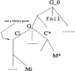
Recall that the distribution P(>.,S, +-mod e l ( M )) over atoms model ( m) is generated by marginalisation from a distribu­ tion of the same name over refutations offmodel(M). Extending our definition to include zero probability imagi­ nary models amounts to extending this underlying distribu­ tion on refutations to also include zero probability SLD­ derivations that end in fail. It turn s out that this last distribution on derivations is the most convenient to work with. Note that each derivation corresponds to a leaf in an SLD-tree. We will associate a leaf corresponding to a failure derivation with fail and a leaf corresponding to a refutation with the model yielded by that refutation. Non­ leaf nodes of the SLD-tree will be associated with goals (see Fig 6).

8.2 The Transition Kernel

We can generate a new derivation (yielding a new proposed model M*) from the derivation which yielded the current model Mi as follows.

1. Backtrack one step to the most recent choice point in the SLD-tree
2. We then probabilistically backtrack as follows: If at the top of the tree stop. Otherwise backtrack one more step to the next choice point with probability p.
3. Use loglinear sampling to generate a derivation from the choice point chosen in previous backtracking step. However, in the first step of sampling we may not choose the branch that leads back to Mi.

If the derivation so found ends in fail then M* is an imaginary model, so p(Mi) = 0, a(Mi, M*) = 0 and we stay at Mi. The parameter p controls the size of steps; if p = 1, we always restart from the top of the tree.

Now, we must calculate a(Mi, M*) when M* turn s out to be a real model. First let G be the deepest common par­ ent goal for Mi and M*. ( Strictly, we should say "for the derivations that yield Mi and M*", but from now on we will abbreviate in this way. ) There is only one way we can get from Mi and M*: backtracking toG and then reaching M* from G. We can not go via some parent of G (such as Go in Fig 6) since we have prohibited going down the tree the same way we backtracked up it.

Suppose that Mi is at depth Ni in the SLD-tree, then the probability of backtracking through n i choice points is p n; -1 (1p) for 1 ::; ni < Ni and p N ; -1 for ni = Ni. Let Bi be the random variable that gives the number of back­ tracks from Mi. Similarly, we have B* for M*. Then we find that P(B* = n*)/P(Bi = ni) = p (n*-n;) whether G is at the top-level choice point or not.

The probability of reaching M* starting from G is '1/J(>.., s , a ) (M*)/(1-l(Ci)) where Ci is the clause which is used at G to get to Mi. So q(Mi, M*) = P(Bi = ni)'I/J (>.,S,G) (M*)[1 -l(Ci)]-1. Swapping i and* sym­ bols gives us q(M*, Mi). The SLD-tree in Fig 6 shows an example, where ni = n* = 2. Note the imag­ inary model under the top-level goal. Next, note that

'1/J (>.,S,Go) (M)/ '1/J(>.., s , a ) (M) is constant for any M below G, since cancelling out the labels of clauses that get us from G toM in '1/J(>..,S,Go) (M) just leaves us with those that get us as far as G. In particular

Finally note that P(>..,S,Go) (M*)/ P(>..,S,Go) (Mi) '1/J (>..,S,Go) (M*)/'1/J(>..,S,Go) (M'), since we are actually deal­ ing with derivations that yield models, and the normalising Z factor cancels out. Putting all this together:

So for real M*, we have

where f(M) is the likelihood of the model: the probability of the observed data given the model, which we assume is at least defined (if not quickly calculable) . Note that we always jump if the following three conditions are met (i) f(M*) 2: f(Mi) (M* fits the data at least as well as Mi), (ii) n* 2: ni (M* is at least as deep as Mi) and (iii) l(C*) 2: l(Ci).

We can propose models quickly since we allow imaginary models. We can also compute the acceptance probability ( 1) easily. The main deficiency is that we may move very slowly through the space of real models if our SLP is highly constrained, leading to slow convergence.

9 Implementation and Experiments

Let us briefly show how SLPs can be implemented in Pro­ Jog, just to see how easy it is. The SLP fragment in Fig 4 is translated to the Pro log code in Fig 7. Each probabilis­ tic predicate gets 3 extra arguments: one is a clause label and the other two (which are hidden in Fig 7 by DCG no­ tation) , are accumulators which pass around a list of the clause labels used and the potential of the derivation. This ugly but efficient implementation can easily by generated by a source-to-source transformation from more aestheti­ cally pleasing code.

theory(main,In,Out) --> select_clause(theory_2,ClauseNum), theory(ClauseNum,In,Out). theory(theory 2 l,Done,NicelyDone) --> { \ + Done = (]} � {nice_all(Done,NicelyDone) }. theory(theory_2_2,RulesSoFar,Done) --> rule (Rule), {newrule(RulesSoFar,Rule)}, !, theory(main, [RuleiRulesSoFar) ,Done). labels(theory_2, [cdp(theory_2_l,O. l,O. l) , cdp(theory_2_2,0.9,1))).

We have yet to do real experiments to test whether our sam­ pling algorithm converges on the true posterior, but at least have a working implementation that is reasonably efficient, and which can be used to explore the consequences of al­ tering various parameters. Running the algorithm with no data (so the likelihoods do not need calculating) using the S4 prior over logic programs took a little over 9 seconds of CP U time to produce (and write out) 10000 samples on a Pentium 233 M Hz running Yap Prolog. This involved 546 acceptances of a proposed M*, an acceptance rate of only 5.46% and involved 337 distinct logic programs. When run using a data set of 5 positive and 5 negative examples and a simple 10% classification noise likelihood function, 10000 samples took 11.5 seconds, involving 451 jumps and 465 distinct logic programs. These runs were done using a backtrack probability of p = 0.8. Reducing p to 0.3 pro­ duced only 39 jumps out of 10000.

10 Conclusions and Future Directions

We have defined a number of algorithms for SLPs, together with relevant mathematical analysis. This goes some way to establishing that SLPs can be a useful framework for rep­ resenting and reasoning with complex probability distribu­ tions. We view the application to Bayesian machine learn­ ing as being the most promising area for future research. The definition of a general-purpose and practical transition kern el is probably the paper' s major contribution. How­ ever, it remains to be proven by rigorous experimentation that our posterior sampler produces better results than more conventional search-based approaches. Also, we have also yet to give a proper account of termination when sampling fromSLPs.

In this paper, we have only considered priors over struc­ tures, not parameters; but it is easy to embed built-in pred­ icates in the Prolog code to generate e. g. samples from a Dirichlet. More interestingly, there is the possibility of combining the likelihood with the prior to generate a pos­ terior in the same form as the prior. It is easy to construct an impractical SLP for the posterior of the form:

posterior (Model) prior(Model), likelihood(Model) .

The interesting question is whether this impractical defini­ tion can be transformed into a usable representation. One problem here, is that the size of an efficient representation of the posterior is likely to explode, given that the posterior is generally more complex than the manually-derived prior.

We conclude by pointing to (Cussens, 2000) where a much more detailed account of SLPs is given, and where the E M algorithm is applied to estimate SLP parameters from data.

Acknowledgments

Special thanks to Blaise Egan for preventing me from re­ inventing the wheel and Gillian Higgins for putting up with me. Thanks also to Stephen Muggleton and Suresh Man­ andhar for useful discussions.

References

Chipman, H. A. , George, E. 1., and McCulloch, R. E. (1998). Bayesian C A RT model search. Journal of the American Statistical Association, 39(443):935-960. with discussion.

Cussens, J. (1999). Loglinear models for first-order prob­ abilistic reasoning. In Proceedings of the Fifteenth Annual Conference on Uncertainty in Artificial Intel­ ligence (UAI-99), pages 126-133, San Francisco, C A. Morgan Kaufmann Publishers.

Cussens, J. (2000). Parameter estimation in stochastic logic programs. Submitted to Machine Learning.

Denison, D. G. T., Mallick, B. K. , and Smith, A. F. M. ( 1998). A Bayesian C A RT algorithm. Biometrika, 85(2):363-377.

Gelman, A., Carlin, J., Stem, H. , and Rubin, D. ( 1995). Bayesian Data Analysis. Chapman & Hall, London.

Muggleton, S. ( 1996). Stochastic logic programs. In de Raedt, L. , editor, Advances in Inductive Logic Pro­ gramming, pages 254-264. lO S Press.

Muggleton, S. (2000). Semantics and derivation for stochastic logic programs. In UAI-2000 Workshop on Fusion of Domain Knowledge with Data for Decision Support.

Riezler, S. ( 1998). Probabilistic Constraint Logic Pro­ gramming. PhD thesis, Universitat Tiibingen. A I M S Report 5(1), 1999, I M S, Universitiit Stuttgart.