Stochastic simulation algorithms for dynamic probabilistic networks

Keiji Kanazawa, Daphne Koller, Stuart Russell

Computer Scjence Division University of California Berkeley, CA 94720, USA

Abstract

Stochastic simulation algorithms such as like­ lihood weighting often give fast, accurate approximations to posterior probabilities in probabilistic networks, and are the methods of choice for very large networks. Unfor­ tunately, the special characteristics of dy­ namic probabilistic networks (DPNs), which are used to represent stochastic temporal pro­ cesses, mean that standard simulation algo­ rithms perform very poorly. In essence, the simulation trials diverge further and further from reality as the process is observed over time. In this paper, we present simulation algorithms that use the evidence observed at each time step to push the set of trials back towards reality. The first algorithm, "evi­ dence reversal" (ER) restructures each time slice of the DPN so that the evidence nodes for the slice become ancestors of the state variables. The second algorithm, called "sur­ vival of the fittest" sampling (SOF), "repop­ ulates" the set of trials at each time step us­ ing a stochastic reproduction rate weighted by the likelihood of the evidence according to each trial. We compare the performance of each algorithm with likelihood weighting on the original network, and also investigate the benefits of combining the ER and SOF methods. The ER/SOF combination appears to maintain bounded error independent of the number of time steps in the simulation.

1 Introduction

Dynamic probabilistic networks or DPNs (Dean and Kanazawa, 1989; Nicholson and Brady, 1992; Kjaerulff, 1992 ) are a species of belief network designed to model stochastic temporal processes.1 They do so by using a section of the network called a time slice to repre-

1 Alternative terms include dynamic belief networks and temporal belief networks.

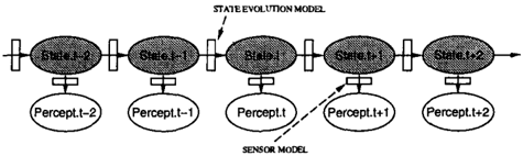
sent a snapshot of the evolving temporal process. The DPN consists of a sequence of time slices where nodes within time slice t are connected to nodes in time slice t + 1 as well as to other nodes within slice t. Figure 1 shows the coarse structure of a generic DPN. The con­ ditional probability tables (CPTs) for a DPN include a state evolution model, which describes the transi­ tion probabilities between states, and a sensor model, which describes the observations that can result from a given state. Typically, one assumes that the CPTs in each slice do not vary over time. The same param­ eters therefore will be duplicated in every time slice in the network.

DPNs serve a number of purposes. They can be used for monitoring a partially observable system-for ex­ ample, Nicholson and Brady used a DPN to track mov­ ing robots using light beam sensors. They can be used to project possible future evolutions of the observed system by adding slices into the future. When deci­ sion nodes are added, they enable approximately ra­ tional decision-making with a limited horizon (Tatman and Shachter, 1990 ) . We have used them for freeway surveillance (Huang et al., 1994 ) and for controlling an autonomous vehicle (Forbes et al., 1995 ) . In this pa­ per, we concentrate on the use of DPNs for monitoring, i.e., maintaining a probability distribution over the possible current states of the world. Since the correct decision in any partially observable environment de­ pends on this distribution (Astrom, 1965 ) , monitoring is also an essential component of embedded decision­ makers.

Exact clustering algorithms for DPNs are described by

Kjaerulff (1992). In our applications, we have found that the clustering approach is too expensive and that exact probabilities are not needed. Furthermore, when continuous variables are included, DPNs seldom con­ form to the structural requirements for CG distribu­ tions (Lauritzen and Wermuth, 1989). Hence, exact algorithms are not available. We have therefore in­ vestigated the use of stochastic simulation algorithms, which often provide fast approximations to the re­ quired probabilities and can be used with arbitrary combinations of discrete and continuous distributions. In the context of DPNs, stochastic simulation meth­ ods attempt to approximate the joint distribution for the current state using a collection of "simulated re­ alities," each describing one possible evolution of the environment.

The simplest simulation algorithm is logic sam­ pling (Henrion, 1988). Logic sampling stochastically instantiates the network, beginning with the root nodes and using the appropriate conditional distribu­ tions to extend the instantiation through the network. Because logic sampling discards trials whenever a vari­ able instantiation conflicts with observed evidence, it is likely to be ineffective in DPN-based monitoring where evidence is observed throughout the temporal sequence.2

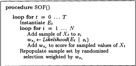
Likelihood weighting (LW) (Fung and Chang, 1989; Shachter and Peot, 1989) attempts to overcome this general problem with logic sampling. Rather than dis­ carding trials that conflict with evidence, each trial is weighted by the probability it assigns to the ob­ served evidence. Probabilities on variables of interest can then be calculated by taking a weighted average of the values generated in the population of trials. It can be shown that likelihood weighting produces an unbi­ ased estimate of the required probabilities. The LW algorithm, which we have adapted for the purposes of maintaining beliefs in a DPN as evidence arrives over time, is shown in Figure 2. We use the notation Et to denote the evidence variables for time slice t, and Xt to denote the state variables for time slice t. N is the number of samples to be generated, s; is the ith sam­ ple, w8, is its weight, and Tis the number of time steps for which the simulation is to be run. Likelihood(Ejs) denotes the product of the individual conditional prob­ abilities for the evidence in E given the sampled values for their parents in s. At each time slice, the current belief for Xt is calculated as the normalized score from the whole sample set.

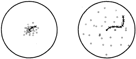
The use of likelihood weighting in DPNs reveals some problems that require special treatment. The difficulty is that a straightforward application generates simu­ lations that simply ignore the observed evidence and therefore become increasingly irrelevant. Consider a simple example: tracking a moving dot on a 2-D sur-

the other hand, logic sampling is extremely effec­ tive for projection, because no evidence is observed in fu­ ture slices.

procedure LIKELIHOOD-WEIGHTING{) loop for i = 1 . . . N w., t-- 1.0 loop for t :::: 0 . . . T Instantiate Et loop for i = 1 . . . N Add sample of Xt to s; Ws; t-Ws; X Likelihood(Et I s;) Add w., to score for sampled values of Xt

face. Suppose that the state evolution model is fairly weak-for example, it models the motion as a random walk-but that the sensor is fairly accurate with a very small Gaussian error. Figure 3 illustrates the difficulty. The samples are evolved according to the state evolu­ tion model, spreading out randomly over the surface, whereas the object moves along some particular trajec­ tory that is unrelated to the sample distribution. The weighting process will assign extremely low weights to almost all of the samples because they disagree with the sensor observations. The estimated distribution will be dominated by a very small number of sam­ ples that are closest to the true state, so the effective number of samples diminishes rapidly over time. This results in large estimation errors. All this occurs de­ spite the fact that the sensors can track the object with almost no error! In the case of traffic surveillance, we have· discovered that a naive application of likelihood weighting results in a large number of more or less imaginary traffic scenes that bear almost no relation to what is actually happening on the road.

Clearly, we need algorithms that use the current sen­ sor values to reposition the sample population closer to reality rather than allowing them to evolve as if no sensor values were available. Section 2 describes a simple method (evidence reversaQ for restructuring the DPN so that likelihood weighting has the desired effect. Section 3 describes a related method (survival of the fittest) that uses the likelihood weights to prefer-

entially propagate the most likely samples, and shows how this can be combined with evidence reversal. Sec­ tion 4 describes an experimental comparison of these techniques with naive LW.

2 Evidence reversal

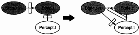
It has long been known that stochastic simulation al­ gorithms are quite effective if the network contains no evidence (Dagum and Luby, 1993). The same argu­ ment can be used to show that if all the evidence in a network is at the root nodes, approximating the prob­ abilities in the rest of the network is computationally tractable. This explains the appeal of logic sampling for projection, but is not directly applicable to the monitoring problem (where evidence is obtained for every time slice). We can force the evidence to be at the root nodes of any network simply by reversing all the arcs using Shachter's (1986) transformations, but doing this to ann-slice DPN results in an exponential blowup. As a compromise, we can do some judiciously selected arc reversals as suggested by Fung and Chang. In the specific case of DPNs, we can take advantage of the fact that each sample, once it instantiates vari­ ables in time slice t -1, d-separates all preceding time slices from the state at timet. We then simply reverse the arcs within slice t, so that the evidence at t and the state at t -1 become the parents of the state at timet. This is shown in schematic form in Figure 4.

The process is then as follows. For each time slice, we have some number k of fully specified states along with their weights.

1. Reverse the arcs from evidence to state at timet; the state variables at time t -1 are now parents of the evidence at timet.
2. Use the evidence at timet to adjust the weights of the samples at timet -1, as in standard likelihood weighting.
3. Propagate each sample at timet1 through the modified state-evolution model which uses the ev­ idence at timet (as obtained in the arc-reversed time slice).

In ER, the current evidence is a parent of the current state; therefore, it can influence the process of extend­ ing the samples to the state variables at t. In partic­ ular, in the 2-D tracking example shown in Figure 3, all the samples will stay closely clustered around the observed position of the object because the accurate sensor readings will dominate the weak state evolution model in the conditional distribution for generating the new samples.

3 Survival of the fittest

The problem with the naive application of sampling algorithms can also be viewed as one of resource allo­ cation. The samples are a constrained resource, and should be allocated in the state space to try to "fit" the actual joint distribution as well as possible. Samples that have wandered off into totally imaginary scenarios should not be propagated, since they do not contribute enough to the estimation of the desired probabilities. The idea of survival-of-the-fittest (SOF) sampling is to preferentially propagate forward in time those samples that have high likelihood for the observed evidence. The SOF process keeps a fixed number of samples, but generates the sample population for time slice t by a weighted random selection from the samples at time t -1, where the weight is given by the likelihood for the evidence observed at time t. This idea is closely related to the use of fitness-related propagation in genetic al­ gorithms and the sample-repositioning method used in randomized "go with the winners" algorithms (Aldous and Vazirani, 1994).

The SOF approach can also be understood as a slice­ by-slice likelihood weighting process. Rather than us­ ing the samples to provide an approximation to the joint probability distribution over the entire (multi­ slice) network, we only use them to propagate the be­ lief state-the joint probability distribution over the state-from one time slice to the next. More precisely, the weighted samples at time t -1 are an approxima­ tion to the belief state at time t -1. We can then use that approximate belief state as our starting point for the sampling at the next time slice. That is, we sample each state according to its weight, as defined by our current (likelihood weighted) samples. These samples are in turn weighted using the evidence at time t , and provide an approximation of the belief state at time t. Note that the probability of sampling a given state at time t is given just by the likelihood for the evidence at timet, and not by the accumulated likelihood for all evidence up to and including time t (as would be the case in standard likelihood weighting). This is because the sample population at timet -1 in SOF already re­ flects the evidence up to timet -1 through the process of preferential propagation. The algorithm is shown in Figure 5.

SOF clearly provides some improvement over likeli­ hood weighting in general, but does not take advan­ tage of the sensor values in quite the same way as ER. In the context of the 2-D tracking problem, SOF will multiply the samples closest to the actual track so that almost the entire population consists of "rea­ sonable" samples and will never spread out over the entire surface. However, the samples will spread out

by an amount related to the uncertainty in the state evolution model, regardless of how accurate the sensor model is. Fortunately, the advantages provided by ER and SOF can be combined into an ER/SOF hybrid, simply by applying SOF to the ER sampling process. That is, rather than propagating all the slice-t -1 sam­ ples at step 3 in the ER algorithm, we use the SOF technique to focus on the ones that are most likely. That is, we sample from the distribution obtained in step 2 of the ER algorithm, and then propagate those through the modified state-evolution model.

4 Empirical results

In this section, we report on some simple experiments we carried out to confirm the intuitive ideas presented above. The network used in our experiments has the same topology as the network shown in Figure 1.3 The aim is to investigate the problem of sample population divergence over time, and to show that ER and SOF mitigate the problem. We measure the average ab­ solute error in the marginal probabilities of the state variables of a time slice as a function oft-that is, the x-axis measures time in the simulated environment.

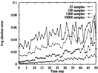
Figure 6 shows the error behaviour for LW over 50 time steps for 25, 100, 1000, and 10000 samples, av­ eraged over 50 randomly generated sets of evidence. The results clearly show that LW fails dramatically even on this very simple network. The problem is that as any given sample is propagated over time, sooner or later it will sample a state value that makes the observed evidence impossible ( for each state value in our network, one of the four observation values in not possible ) . After sufficiently many steps, all the sam­ ples end up with weight 0, at which point we assign an error of 1.0. Thus, after 39 steps with 25 samples, all the samples are extinguished in all 50 cases. Multiply­ ing the number of samples only delays the inevitable by a small number of steps.

Figure 7 shows the corresponding error behaviour for ER. Note that the scale of the y-axis is increased by 10. Thus, the error remains well within the acceptable

3We are currently working to generate similar experi­ mental data for our traffic surveillance networks.

range. It does, however, show a slow increase over time. It is possible that the error asymptotes as t -t oo, but we have not yet run those experiments.

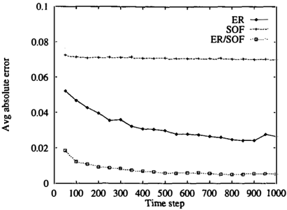
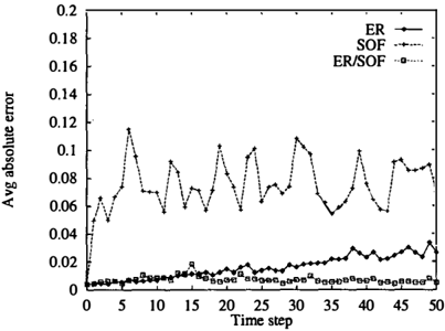
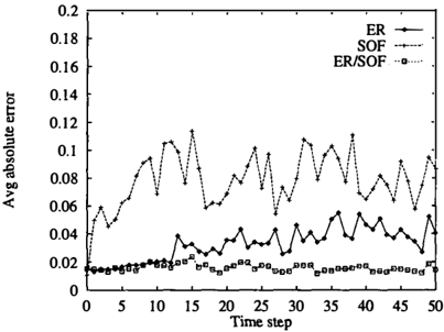
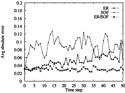
Figures 8, 9, and 10 show the performance of SOF and ER/SOF, compared with ER, for 25, 100, and 1000 samples respectively. The results show that SOF is an effective mechanism for maintaining bounded error over time. Although SOF on its own shows somewhat higher error than ER, as one would expect, the com­ bination of ER and SOF shows low error for all time steps and shows no sign of diverging at all.

Finally, Figure 11 shows the performance of ER, SOF, and ER/SOF as a function of the number of samples for the range 50 to 1000 samples. The graph gives the average absolute error in the marginal probabili­ ties of the state variable at t = 50. The graphs show that SOF seems to benefit much less from additional samples than ER-in fact, the curve is almost flat. Currently, our theoretical analysis of the algorithm is not sufficiently advanced to explain this phenomenon.

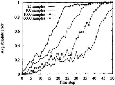
Figure 8: Performance of ER, SOF, and ER/SOF: Graph showing the average absolute error in the marginal proba­ bilities of the state variables of a time slice as a function of t, averaged over 50 randomly generated evidence cases, for 25 samples.

L-�--��--�-�

5 Conclusion and further work

We have presented two very simple and intuitive im­ provements that make the likelihood weighting tech­ nique effective for dynamic probabilistic networks. Early experimental results confirm our intuitions. In particular, the error for SOF and ER/SOF seems to be independent of the number of time steps in the simu­ lation. This is an absolute requirement for monitoring applications such as traffic surveillance, where infer­ ence continues over many days of real time.

Further work needs to be done to establish the theoret­ ical properties of the algorithms. The most obvious is­ sue is whether these approaches are unbiased: do they converge to the right answer as the number of samples grows to infinity. ER is clearly unbiased, because it just an application of likelihood weighting to a modi­ fied network structure. It seems fairly straightforward to show that SOF (and therefore ER/SOF) converge to the correct values in the large-sample limit using standard probabilistic techniques.

We would also like to investigate the expected error as a function of sample size for LW, ER, SOF, and ER/SOF. This should be fairly simple for specific net­ work structures such as that shown in Figure 1. Under­ standing the algorithms' behaviour for general DPNs is more difficult. Intuitively, the improvement of ER and SOF is more pronounced in those cases where the evidence gives us a lot of information about the state. At one extreme, if the sensor model is completely accu­ rate, ER will be completely accurate with only a single sample. The behavior of SOF in these circumstances will also depend on the behavior of the state-evolution model. If this is fairly well-behaved, it appears that SOF will also do well. At the other extreme, if the sensor model is just noise, neither approach seems to provide an advantage over LW. We hope to analyze the improvement of these algorithms using such quan­ tities as (1) the distance (in terms of relative entropy)

between the belief-state distribution at time t and at timet+ 1, and (2) the amount of information ( in terms of entropy ) obtained by considering the sensors.

Finally, SOF is a technique that can be applied to arbi­ trary networks, not just DPNs. It would be interesting to see if it provides consistently better results than LW for general networks. Since LW is currently the best algorithm known for very large networks, this would be a useful development.

References

David Aldous and Umesh Vazirani. "go with the win­ ners" algorithms. In Proceedings 35th Annual Sym­ posium on Foundations of Computer Science, pages 492-501, Santa Fe, New Mexico, November 1994. IEEE Computer Society Press.

1. J. Astrom. Optimal control of Markov de­ cision processes with incomplete state estimation. J. Math. Anal. Applic., 10:174-205, 1965.
2. Dagum and M. Luby. Approximating probabilis­ tic inference in Bayesian belief networks is NP-hard. Artificial Intelligence, 60(1):141-153, March 1993.

Thomas Dean and Keiji Kanazawa. A model for rea­ soning about persistence and causation. Computa­ tional Intelligence, 5(3):142-150, 1989.

• Jeff Forbes, Tim Huang, Keiji Kanazawa, and Stu­ art Russell. The BATmobile: Towards a Bayesian automated taxi. Submitted to IJCAI-95, 1995.
• Fung and K. C. Chang. Weighting and integrating evidence for stochastic simulation in Bayesian net­ works. In Proceedings of the Fifth Conference on Un­ certainty in Artificial Intelligence (UAI-89), Wind­ sor, Ontario, 1989. Morgan Kaufmann.

Max Henrion. Propagation of uncertainty in Bayesian networks by probabilistic logic sampling. In John F. Lemmer and Laveen N. Kana}, editors, Uncer­ tainty in Artificial Intelligence 2, pages 149-163. Elsevier/North-Holland, Amsterdam, London, New York, 1988.

1. Huang, D. Koller, J. Malik, G. Ogasawara, B. Rao, S. Russell, and J. Weber. Automatic symbolic traffic scene analysis using belief networks. In Proceedings of the Twelfth National Conference on Artificial Intelli­ gence ( AAAI-94), Seattle, Washington, 1994. AAAI Press.
2. Kjaerulff. A computational scheme for reasoning in dynamic probabilistic networks. In Proceedings of the Eighth Conference on Uncertainty in Artificial In­ telligence, pages 121-129, 1992.
3. L. Lauritzen and N. Wermuth. Graphical models for associations between variables, some of which are qualitative and some quantitative. Annals of Statis­ tics, 17:31-57, 1989.
4. E. Nicholson and J. M. Brady. The data asso­ ciation problem when monitoring robot vehicles us-
5. ing dynamic belief networks. In EGA! 92: 10th Eu­ ropean Conference on Artificial Intelligence Proceed­ ings, pages 689-693, Vienna, Austria, 3-7 August 1992. Wiley.
6. D. Shachter and M. A. Peot. Simulation ap­ proaches to general probabilistic inference on belief networks. In Proceedings of the Fifth Conference on Uncertainty in Artificial Intelligence (UAI-89}, Windsor, Ontario, 1989. Morgan Kaufmann.
7. Ross D. Shachter. Evaluating influence diagrams. Op­ erations Research, 34:871-882, 1986.
8. A. Tatman and R. D. Shachter. Dynamic pro­ gramming and influence diagrams. IEEE Transac­ tions on Systems, Man and Cybernetics, 20(2) :365379, March-April 1990.