Structure-Based Causes and Explanations in the Independent Choice Logic

Alberto Finzi and Thomas Lukasiewicz* Dipartimento di Informatica e Sistemistica, Universita di Roma "La Sapienza" Via Salaria 113, I-00198 Rome, Italy { finzi, Iukasiewicz } @dis.uniromal.it

Abstract

This paper is directed towards combining Pearl's structural-model approach to causal reasoning with high-level formalisms for reasoning about actions. More precisely, we present a combi­ nation of Pearl's structural-model approach with Poole's independent choice logic. We show how probabilistic theories in the independent choice logic can be mapped to probabilistic causal models. This mapping provides the independent choice logic with appealing concepts of causal­ ity and explanation from the structural-model approach. We illustrate this along Halpern and Pearl's sophisticated notions of actual cause, ex­ planation, and partial explanation. This mapping also adds first-order modeling capabilities and explicit actions to the structural-model approach.

1 INTRODUCTION

Handling causality is an important issue, which emerges in many applications in AI. The existing approaches to causal­ ity in the AI literature can be roughly divided into those that have been developed as modal nonmonotonic logics ( espe­ cially in the context of logic programming) and those that evolved from the area of Bayesian networks. A represen­ tative of the former is Geffner's modal nonmonotonic logic for handling causal knowledge [14, 15], which has been inspired by default reasoning from conditional knowledge bases. More specialized modal-logic based formalisms play an important role in dealing with causal knowledge about actions and change; see especially the work by Turner [36] and the references therein for an overview. A representative of the latter is Pearl's approach to modeling causality by structural equations [2, 12, 28, 29], which is central to a number of recent research efforts. In particular,

'Alternate address: Institut fiir Informationssysteme, Tech­ nische Universitat Wien, FavoritenstraBe 9-11, A-1040 Vienna, Austria; e-mail: [email protected].

the evaluation of deterministic and probabilistic counter­ factuals has been explored, which is at the core of problems in fault diagnosis, planning, decision making, and determi­ nation of liability [2]. It has been shown that the structural­ model approach allows a precise modeling of many impor­ tant causal relationships, which can especially be used in natural language processing [ 12]. An axiomatization of reasoning about causal formulas in the structural-model ap­ proach has been given by Halpern [ 16].

Concepts of causality also play an important role in the generation of explanations, which are of crucial importance in areas like planning, diagnosis, natural language process­ ing, and probabilistic inference. Different notions of expla­ nations have been studied quite extensively, see especially [19, 13, 34] for philosophical work, and [27, 35, 20] for work in AI that is related to Bayesian networks. A criti­ cal examination of such approaches from the viewpoint of explanations in probabilistic systems is given in [6].

In recent papers [17, 18], Halpern and Pearl formalized causality using a model-based definition, which allows for a precise modeling of many important causal relationships. Using a notion of weak cause, they propose appealing defi­ nitions of actual cause [17] and of causal explanation [18]. As they show, their notions of actual cause and causal explanation, which is very different from the concept of causal explanation in [24, 26, 14], models well many prob­ lematic examples in the literature. As for computation, Biter and Lukasiewicz [7, 8, 9] analyzed the complexity of these notions and identified tractable cases, and Hop­ kins [21] explored search-based strategies for computing actual causes in the general and restricted settings.

However, structural causal models, and thus also the above notions of actual cause and causal explanation, have only a limited expressiveness in the sense that (i) they do not allow for first-order modeling, and (ii) they only allow for explic­ itly setting the values of endogenous variables (also called an intervention) as actions, but not for explicit actions as in well-known formalisms for reasoning about actions.

There are a number of formalisms for probabilistic reason-

ing about actions. In particular, Bacchus et al. [I] propose a probabilistic generalization of the situation calculus, which is based on first-order logics of probability, and which al­ lows one to reason about an agent's probabilistic degrees of belief and how these beliefs change when actions are exe­ cuted. Poole's independent choice logic [30, 31] is based on acyclic logic programs under different "choices". Each choice along with the acyclic logic program produces a first-order model. By placing a probability distribution over the different choices, one then obtains a distribution over the set of first-order models. Other probabilistic extensions of the situation calculus are given in [25, II]. A probabilis­ tic extension of the action language A is given in [3].

The main idea behind this paper is to develop a combi­ nation of Pearl's structural-model approach to (probabilis­ tic) causal reasoning with high-level formalisms for (prob­ abilistic) reasoning about actions. To this end, we present a combination of Pearl's structural-model approach with Poole's independent choice logic. We show how proba­ bilistic theories in the independent choice logic [30, 31] can be translated into probabilistic causal models. This translation provides the independent choice logic with ap­ pealing concepts of causality and explanation from the structural-model approach. We illustrate this along Halpern and Pearl's notions of actual cause and causal explanation. This mapping also adds first-order modeling capabilities and explicit actions to the structural-model approach.

The work closest in spirit to this paper is perhaps the re­ cent one by Hopkins and Pearl [22], which combines the situation calculus [33] with the structural model-approach. However, the generated causal models are much differ­ ent from the ones in this paper. First, and as a central conceptual difference, Hopkins and Pearl consider a stan­ dard situation calculus formalization, which allows for ex­ pressing uncertainty about the initial situation, but which does not allow for uncertain effects of actions. In this pa­ per, however, we consider Poole's independent choice logic [30, 31], which is a first-order formalism that allows both for probabilistic uncertainty about the initial situation and about the effects of actions. Second, the work [22] focuses only on counterfactual and probabilistic counterfactual rea­ soning, while our work here extends the notions of actual cause, explanation, and partial explanation to the indepen­ dent choice logic. Third, [22] focuses only on hypothetical reasoning about subsequences of an initially fixed sequence of actions, while our approach here basically allows for hy­ pothetical reasoning about any actions and fluent values.

Note that also Poole [32] defines a notion of explanation for his independent choice logic. However, Poole's no­ tion of explanation in [32] is based on abductive reason­ ing and assumes that explanations are defined over choice atoms. Our notion of explanation in this paper, in contrast, is based on causal reasoning in structural causal models, and assumes that explanations are defined over endogenous variables. Hence, our concept of explanation here is con­ ceptually much different from the one by Poole in [32].

2 CAUSAL MODELS

In this section, we recall some basic concepts from Pearl's structural-model approach to causality [2, 12, 28, 29]. In particular, we recall causal and probabilistic causal models.

2.1 PRELIMINARIES

We assume a set of random variables. Every variable Xi may take on values from a nonempty domain D(Xi)· A value for a set of variables X is a mapping x that associates with each Xi EX an element of D(Xi) (for X= 0, the unique value is the empty mapping 0). The domain of X, denoted D(X), is the set of all values for X. For Yt;X and x E D(X), denote by xiY the restriction of x toY. For disjoint sets of variables X, Y, and values x E D(X), y E D(Y), denote by xy the union of x andy. We often identify singletons {Xi} with Xi, and their values x with x (Xi ) .

2.2 CAUSAL MODELS

A causal model M = (U, V, F) consists of two disjoint sets U and V of exogenous and endogenous variables, respectively, and a set F = {Fx I X E V } of functions Fx: D(P Ax )--+ D(X) that assign a value of X to each value of the parents PAx c; U U V \ {X} of X. The val­ ues u E D(U) are also called contexts. A probabilistic causal model M = ((U, V, F), P) consists of a causal model (U, V, F) and a probability function P on D(U).

We focus here on the principal class [17] of recursive causal models M = (U, V, F) in which a total ordering -< on V exists such that Y E PAx implies Y-< X, for all X, Y E V . In such models, every assignment to the ex­ ogenous variables U = u determines a unique value y for every set of endogenous variables Y c; V, denoted YM(u) (or simply Y ( u ) ). For any causal model M = (U, V, F), set of variables X c; V, and value x E D(X), the causal model Mx=x = (U, V\X, Fx =x), where Fx=x = {F� I Y E V \ X} and each F� is obtained from Fy by setting X to x, is a submodel of M. We abbreviate Mx=x and Fx =x by Mx and Fx, respectively. For Y c; V, we abbreviate YM. ( u) by Y x(u) . A causal or probabilistic causal model is binary iff I D(X)I = 2 for all endogenous variables X.

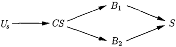
Example 2.1 (stopping robot) Suppose a mobile robot de­ tects the presence of an obstacle. Then, the command stop is executed by the control system, which activates two brakes 1 and 2 (wheels behind and ahead), and the robot stops. The robot can stop using only one of the two brakes.

This scenario can be modeled by the following recursive causal model M = (U, V, F). The exogenous variables are given by U = {U8}, where D(Us) = {0, 1}, and U8 is 1 iff

an obstacle has been detected. The endogenous variables are given by V = {CS,B1,B2,S}, where D(X) = {0, 1} for all X E V, CS is 1 iff the command stop is executed, Bi is 1 iff brake i is activated, and S is 1 iff the robot stops. The functions F = { Fx I X E V} are given by Fcs = U5, Fs, = Fs, = CS, and Fs = 1 iff B 1 = 1 V B2 = 1. Fig. I shows the parent relationships between the variables.

The submodel Ms,=o=(U, Vs,=o, Fs,=o) is given by Vs,=o={CS,Bt,S} and Fs,=o={Fb5=Fcs, Fl,,= Fs, F�=1 iff B 1 = 1 }. Then, Ss,=o(Us = 1) = 1.

A probabilistic causal model (M, P) may then be given by the additional probability function P on D(U) defined by P(Us = 1) = 0.7 and P(Us = 0) = 0.3. D

3 INDEPENDENT CHOICE LOGIC

In this section, we recall Poole's independent choice logic (ICL) [30, 31, 32]. We first recall a many-sorted first-order language of logic programs, which are given a semantics in Herbrand interpretations. We then recall the ICL itself.

3.1 PRELIMINARIES

Let if> be a many-sorted first-order vocabulary with the sorts object, time, and action. Let if> contain function sym­ bols of the sort object k -t object, the function symbols 0 and + 1 of the sorts time and time -t time, respectively, and function symbols of the sort object k -taction, where k 2': 0. We call them object, time, and action symbols, re­ spectively. As usual, constant symbols are 0-ary function symbols. Let if> also contain predicate symbols of the sort object k x time, where k 2: 0, and the predicate symbol do of the sort action x time. We call them .fluent and action predicate symbols, respectively. Let X be a set of variables, which are divided into object, time, and action variables.

An object term is either an object variable from X or an expression of the form f(t1, ... ,tk), where f is a k-ary object symbol, and t1, ... , tk are object terms. A time term is either a time variable from X, or the time symbol 0, or an expression of the form s+ 1, where s is a time term. We use 1, 2, . . . to abbreviate 0+ 1, 0+ 1 + 1, . . . . An action term is either an action variable from X, or an expression of the form a(t1, ... , tk). where a is a k-ary action sym­ bol, and t1, ... , tk are object terms.

We define formulas by induction as follows. The proposi­ tional constants false and true, denoted l_ and T, respec- tively, are formulas. Atomic formulas (or atoms) are of the form d o ( a , s) or p ( t t , ... ,tk.s), where a is an action term, s is a time term, p is a k-ary fluent predicate symbol, and t1, ... , tk are object terms. We call them action atoms and fluent atoms (or simply actions and fluents), respec­ tively. If¢ and 7j; are formulas, then also �¢and ( ¢1\ 7j; ) . We use ( ¢ V 7j;) and ( ¢ <r7j;) to abbreviate � ( �¢ 1\ � ¢) and �( �¢ 1\ 7j;), respectively, and adopt the usual conven­ tions to eliminate parentheses. A clause is a formula of the form¢¢=7j;, where¢ (resp., 7j;) is an atom (resp., for­ mula) called its head (resp., body).

Terms and formulas are ground iff they do not contain any variables. Substitutions, ground substitutions, and ground instances of terms and formulas are defined as usual.

We use HB <I! (resp., HU <I!) to denote the Herbrand base (resp., Herbrand universe) over if>. A world I is a subset of HB <I!. We use I<11 to denote the set of all worlds over if>. A variable assignment a maps every variable from X to an element of HU <I! of appropriate sort. It is extended to object, time, and action terms as usual. The truth of formu­ las¢ in I under a, denoted I f=u ¢, is defined by induction as follows (we write I f= ¢ when ¢ is ground):

• I Fu do(a, s) iff do(a(a), a(s)) E I;
• I Fu p(t1, ... , tk) iffp(a(ti ), ... ,a(tk)) E I;
• I Fu � ¢ iff not I f=u ¢;
• I Fu (¢ 1\ ¢)iff I f=u ¢and I Fu 7f;.

A world I is a model of a set of formulas F, denoted I f= F, iff I Fu F for all FE F and all a.

3.2 INDEPENDENT CHOICE LOGIC

A choice space C is a set of pairwise disjoint and non empty sets A <;:: HB <I!. The members of C are called its alterna­ tives and their elements atomic choices. A total choice of Cis a set B <;:: HB<I! such that IE n AI= 1 for all A E C. A probability P on a choice space C is a probability function on the set of all total choices of C. If C and all its alter­ natives are finite, then P can be defined by (i) a mapping P: U C--'> [0, 1] such that LaE A P(a) = 1 for all A E C, and (ii) P(B) = lhEsP(b) for all total choices B of C.

A logic program Lis a set of clauses. We use ground(L) to denote the set of all ground instances of clauses in L. A logic program is acyclic iff a mapping"' from HB<I! to the non-negative integers exists such that K(p) > K(q) for all p, q E HB<I! where p (resp., q) occurs in the head (resp., body) of some clause in ground(L). The answer set (or stable model) of an acyclic logic program L is a world I such that for every p E HB <I!, it holds that I f= p iff I f= 7j; for some clause p <r7j; in ground(L).

An independent choice logic theory (or ICL-theory) T = ( C, L) consists of a choice space C, and an acyclic logic program L such that no atomic choice in C coincides

with the head of any clause in ground(£). A probabilis­ tic ICL-theory (or PICL-theory) T = ((C, L), P) consists of an ICL-theory (C, L) and a probability P on C.

We next define the semantics of ICL- and PICL-theories by associating with them certain worlds and a probability distribution on certain worlds, respectively. A world I is a model of an ICL-theory T = ( C, L ) , denoted If= T, iff I is an answer set of L U {p ¢= T I p E B} for some total choice B of C. In a PICL-theory T = ( ( C, L), P), the probability of such a world I is then defined as P(B).

The following example illustrates how action descrip­ tions and probabilistic action descriptions can be encoded in ICL- and PICL-theories, respectively.

Example 3.1 (mobile robot) Consider a mobile robot, which can navigate in an environment and pick up objects. We assume the constants r1 (robot), o1 (object), p1,P2 (po­ sitions), and 0 (time). The domain is described by the flu­ ents carrying(O, T) and at(X, Pos, T), where 0 E { o l} , XEb,o!}, PosE{pl,P2}, and TE{O,l, ... }. Here, carrying(o, t) and at(x,p, t) mean that the robot r1 is car­ rying the object o at time point t and that the robot or object x is at position p at time point t, respectively. The robot is endowed with the actions moveTo(Pos), pickUp(O), and putDown(O), where PosE {p!,P2} and 0 E { o l } . Here, moveTo(p), pickUp(o), and putDown(o) represent the actions "move to the position p", "pick up the ob­ ject o", and "put down the object o", respectively. The action pickUp(o) is stochastic: It is not reliable, and thus can fail. Furthermore, we have the predicates do(A, T), which represents the execution of an action A at time T, and fa(A, T) (resp., su(A, T)), which represents the fail­ ure (resp., success) of an action A executed at time T. An ICL-theory ( C, L) is then given by the choice space C = { {fa1=fa(pickUp(ol), t), SUt=su(pickUp(ol), t)} I t E {0, 1}} and the following logic program L:

carrying(O, T+1) ¢= at(r1, Pas, T) II at(O, Pos, T) II do(pickUp(O), T) II su(pickUp(O), T);

carrying ( 0, T +I) ¢= carrying ( 0, T) II -,do(putDown(O), T);

at(r1, Pos, T+l) ¢= do(moveTo(Pos), T);

at(r1, Pos, T+1) at(r1, Pos, T)

¢= II -,do(moveTo(Posl), T) II Posl f Pos;

at(O, Pas, T +1) ¢= at(O, Pos, T)ll-,carrying(O, T);

at(O, Pas, T+l) ¢= carrying(O, T) II do(moveTo(Pos), T);

at(O, Pos, T+l) ¢= at(O, Pos, T) II -,do(moveTo(Pos1), T) II Pos1 f Pos;

at( o 1, P 2, 0 ) ¢= T; at(r1,P2,0) ¢= T.

A PICL-theory ((C,L),P) is given by P({fa0,su1}) = P({suo,Ja1}) = 0.21, P({fa0,Ja1 }) =0.09, and P({suo, su1 }) = 0.49, which is obtained from P(fa0) = P(fa1) = 0.3 and P(su0) = P(su1) = 0.7 by assuming probabilistic independence between {fa0, suo} and {fa1, sud. 0

4 TRANSLATIONS

In this section, we first give a translation of PICL-theories into probabilistic causal models. We then show how action executions at different time points can be included into this translation. We finally also provide a converse translation of binary probabilistic causal models into PICL-theories.

4.1 FROM ICL TO CAUSAL MODELS

We now define a translation of PICL-theories ( ( C, L), P) into probabilistic causal models. The main idea behind it is to use (i) each alternative A of the choice space C as an exogenous variable with the set of all atomic choices of A as domain, and (ii) each other ground atom as an endoge­ nous variable with binary domain, where the functions are specified by the clauses of the acyclic logic program L.

In the sequel, let T = ( ( C, L), P) be a PICL-theory. The probabilistic causal model associated with T, denoted My= ((Uy, Vy, Fy ), P y ) , is defined as follows:

• Uy = C, where D(A) = A for all A E C.
• Vy = HB<I>\U C, where D(Vi)={l.,T} for all ViEVy.
• Fy = { Fp I p E Vy}, where PAp is the set of all ground atoms that occur in the body of some p ¢= 1/J in ground ( L), and for every v E D(PAv) we define Fp(v) =Tiff v f= 1/J for some p ¢= 1/J in ground(£). Notice that then Fp = l. for all ground atoms p in no head of a clause in ground ( L).
• Py(u) = P( { u (A) I A E C}) for all u E D(U).

For ICL-theories T = ( C, L), the causal model associated with T, denoted My, is defined as the above (Uy, Vy, Fy ) . Given a total choice B for C, we define un E D(Uy) by un(A) E B n A for all A E Uy=C. The following ex­ ample illustrates the above translation of PICL-theories into probabilistic causal models.

Example 4.1 (mobile robot (continued)) Consider the PICL-theory T = ( ( C, L), P) given in Example 3.1. Its as­ sociated probabilistic causal model My= ((Uy, Vy, Fy ), Py) is given as follows. The exogenous variables are given by Uy = {Uo, Ul}, where Uo = {fa0, suo}= D(Uo) and U1 = {fa1, su1} = D(U1 ) . The endogenous variables Vy are given by all the ground atoms that do not oc­ cur in Uy, where D(X) = {1., T} for all X E V y. For example, the ground atoms carrying(oi,O), at(rl,P l, 1), do(moveTo(p1),0), and do(pickUp(o1), 1) are all in Vy. The functions F y = { F v I p E V } are as specified above. For example, Fat ( r,,p,,l)=T iff either do(moveTo(p l), O)=T, or at(r1,p1,0)=T and do(moveTo(p2),0)=l.. Finally, Py is defined by Py(u)= P(Bu) for all u E D(U), where Bu is the total choice associated with u. For exam­ ple, PT(Uo = fa0, U1 = fa1)= P({fa0,fa1}) = 0.09. o

4.2 ACTION EXECUTION SETS

We next describe how action executions at different time points in ICL can be incorporated into the probabilistic causal model Mr associated with a PICL-theory T.

We define an action execution set E as a set of ground atoms of the form do( a, t). Intuitively, E represents the following set of action executions: For every do( a, t) E E, the action a is executed at time point t.

Example 4.2 (mobile robot (continued)) An action exe­ cution set for the PICL-theory of Example 3.1 is given by E= {do(moveTo(p1),0), do(pickUp(ol), 1 )} , which represents the execution of the actions "move to p1" and "pick up o1" at time points 0 and 1, respectively. 0

In the sequel, letT= ( ( C, L), P) be a PICL-theory. A.n ac­ tion execution set E can be taken into consideration in Mr either (I) by additionally expressing the elements of E as clauses in Land then generating Mr, or (2) by considering the submodel of Mr in which the elements of E are explic­ itly set to T. More formally, the probabilistic causal model M = ( (U, V, F), P) forT and E are defined as follows:

• (I) We define M as MT', where T' = ((e, LU {e <= T I e E E}), P). Then, the executions in E can be over­ ridden by explicitly setting them in M (for example, in counterfactual reasoning).
• We define M as (Mr)E=(Mr)E=e· where e E D(E) is defined by e(X) = T for all X E E. Then, the executions in E are fixed in M: They do not occur in M and thus cannot be changed anymore.

Since from a technical viewpoint, (I) is a special case of (2), we consider only (2) in the rest of this paper. The following example illustrates (I) and (2).

Example 4.3 (mobile robot (continued)) Consider the PICL-theory T = ( ( e , L ) , P) given in Example 3.1, and the action execution set E given in Example 4.2. Un­ der the representation (I), we then obtain the probabilis­ tic causal model Mr·, where T'=((e,L'),P) and L'= LU {do(moveTo(pl),O) <= T,do(pickUp(o1), 1) <= T}. Here, alternative executions can be explored by considering submodels that are obtained from Mr· by explicitly setting the values of do(moveTo(p1),0) and do(pickUp(ol), 1), for example, to l_ and T, respectively. Under (2), we obtain the causal model (Mr)E =(Mr)E=eo where e(X)= T for all X E E. Here, the action executions in E are fixed and cannot be changed anymore. 0

4.3 FROM CAUSAL MODELS TO ICL

We finally also provide a converse translation of binary probabilistic causal models M = ((U, V, F), P) into PICL­ theories. The main ideas behind it are (i) to use the domains of the exogenous variables in U as alternatives in the choice space, and (ii) to represent the functions in F as clauses in an acyclic logic program under the answer set semantics.

In the sequel, let M = ( (U, V, F), P) be a binary probab­ ilistic causal model, where D(X) = {0, 1 } for all X E V , F = {Fx I X E V }, and PAx is finite for every X E V . The PICL-theory associated with M, denoted TM = ( (eM, L M), PM), is then defined as follows:

• eM= { {ui = ui 1 ui E D(Ui)} 1 ui E u};
• LM={X =1 <= ¢i I X EV, i EI}, where ¢ i , for every in­ dex i E J, is a conjunction of assignments Y = y, such that (i) Y E PAx, (ii) y E D(Y), and (iii) for all p E D(PAx ) , it holds that V i E I ¢ i is true in p iff Fx (p) = 1;
• PM(B)=P({(Ui,ui) IUi=UiEB}) for every total choice B of eM.

Fer bin�ry causal models }.1 = (U, ll, F), the ICL-theory associated with M, denoted T M, is defined as the above (eM, L M). The following example illustrates the transla­ tion of probabilistic causal models into PICL-theories.

Example 4.4 (stopping robot (continued)) Consider again the probabilistic causal model M=((U,V,F),P) given in Example 2.1. Its associated PICL-theory TM = ((eM, L M ), PM) is given as follows. The choice space is given by eM= { {Us=1, Us =O} }. The acyclic logic pro­ gram L M is given by the following clauses:

Finally, the probability function PM on C M 's total choices c1 ={Us = 1 } and Cz = {Us= 0} is defined by PM(cl) = P(Us = 1) and PM(c2) = P(Us = 0). 0

5 WEAK AND ACTUAL CAUSES

In this section, we extend the notions of weak and actual cause by Halpern and Pearl [ 17] to ICL-theories. Infor­ mally, the main idea behind this extension is to define weak and actual causes in ICL-theories T as weak and actual causes in their associated causal models M T.

Observe that even though [ 17] defines the notions of weak and actual cause only for the restricted case of a finite num­ ber of endogenous variables, the extended version of [ 17] also describes how these notions can be generalized to the infinite case. It also gives an example, which deals with in­ finite weak and actual causes, where such a generalization is necessary. In the sequel, we consider only the original definitions from [ 17], and we disallow infinite weak and actual causes, to avoid the above-mentioned problems.

We first recall weak and actual causes from [17]. A primi­ tive event is an expression Y = y, where Y is a variable and y is a value for Y. The set of events is the closure of the set of primitive events under the Boolean operators .., and 11. The truth of an event¢ in M = (U, V, F) under u E D(U), denoted (M, u) f= ¢, is inductively defined by:

• (M,u) f= Y =y iffY M (u) = y;
• (M, u) f= · ¢ iff (M, u) f= ¢does not hold;
• (M, u) f= ¢/1 'ljJ iff (M, u) f= ¢and (M, u) f= '1/J.

We use ¢(u) to abbreviate (M, u) f= ¢. For X� V and x E D(X), we use r/!x(u) to abbreviate (Mx, u) p ¢. For X={X1, . . . ,Xk}�V with k2':1 and X iE D ( X i ) , we use X= x1 · · · Xk to abbreviate X1 = x1 /1 . . . /1 Xk =Xk.

Let M = (U, V, F) be a causal model. Let X s V and x E D(X), and let ¢ be an event. Then, X= x is a weak cause of¢ under u iff the following conditions hold:

AC2. Some set of variables W�V\X and some values xED(X), wED(W) exist such that (a) ·rf>xw(u), and (b) rPxwz(u) for all Z � V \(XU W) and z = Z ( u) .

Moreover, X = x is an actual cause of¢ under u iff addi­ tionally the following condition is satisfied:

AC3. X is minimal. That is, no proper subset of X satis­ fies both ACI and AC2.

We are now ready to define the notions of weak and actual cause for ICL-theories as follows.

Definition 5.1 Let T = ( C, L) be an ICL-theory, 'ljJ be a conjunction of atoms, and ¢ be a formula. Let B be a total choice for C, and E be an execution set. Then, 'ljJ is a weak (resp., an actual) cause of¢ under B and E in T iff p( 'lj;(}) is a weak (resp., an actual) cause of p( rj!(}) under us in (MT ) E for each ground substitution(}, where p(5) is ob­ tained from 5 by replacing every ground atom p by p = T.

Example 5.1 (mobile robot (continued)) Consider again the mobile robot scenario described in Example 3.1. Suppose now that there are two objects o1 and 02, and that the robot r1 cannot hold them both in the same time. Consider the ICL-theory T = ( C, L ) , where the choice space is given by C = { {fao,t = fa(pickUp(o), t), suo,t = su(pickUp(o), t)} I o E { 01, 02}, t E {0, 1, 2} }, and Lis given as in Example 3.1 except that the first clause is replaced by the following two clauses:

Assume that executing a pickup succeeds at every time point t E {0, 1, 2}, which is represented by the total choice B = { su0,t I o E { 01, 02}, t E {0, 1, 2} }, and that the robot r1 executes a pickup of 01 at time point 0, a move to P1 at time point 1, and a pickup of o2 at time point 2, which is expressed by the action execution set E = { do(pickUp(ol), 0), do(moveTo(pl), 1), do(pickUp(o2), 2)}. We now show that o1 being at position P2 at time point 0 is an actual cause of the robot not carrying o2 at time point 2, that is, that 'ljJ = at ( o1 , p2, 0) is an actual cause of rjJ ·carrying(o2, 2) under Band E in T.

We show that at(o1,p2,0)=T is [In actual cause of carrying(o2, 2)=.L under us in (MT )E=(U, V, F). Obvi· ously, at(o1,p2,0)(us) =T and carrying(o2,2)(us) = .L in (MT)E· That is, (ACI) holds. Consider next X={at(o1,P2,0)}, x={(at(o1,p2,0), T)}, X'={(at(o1, P2,0),.L)}, W = {at(o2,p1,t) I tE{0,1,2, ... }}, and w = {(Wi, T) I wi E W}. We then obtain carrying(o2, 2)xw (us) = T. That is, (AC2) (a) holds. Furthermore, we obtain carrying(o2, 2)xw(us)=.L and Zxw(us)=Z(us) for Z = V\ ( XUW) (setting W = w and thus inverting at(o2,p1, t) fortE {0, 1, 2, . .. } does not affect other flu· ents). That is, also (AC2) (b) holds. This shows that at(o1,p2,0) = T is a weak cause of carrying(o2,2) =.L under us in (MT ) E. Since X is a singleton, also (AC3) holds. It thus follows that at(o1 ,p2, 0) = T is also an ac· tual cause of carrying(o2, 2) =.Lunder us in (MT )E. 0

The next example shows that we can also refer to the actu· ally executed actions in weak and actual causes, if we make use of representation (I) for action execution sets.

Example 5.2 (waiting collector) We consider a simplified version of Example 3.1, where (i) we have only the fluent carrying(T) with T E {0, 1, ... } and the two actions wait and pickUp, and (ii) we assume that the action pickUp can fail or succeed (which depends on the time point of the execution of pickUp). Consider the ICL­ theory T = ( C, L), where the choice space is given by C={{su(pickUp,t),fa(pickUp,t)}1tE{0,1}}, and L describes the dynamics of this simple scenario by means of the following two clauses:

Assume that executing a pickup succeeds at time point 0, but fails at time point 1, which is represented by the to­ tal choice B = {fa(pickUp, 1), su(pickUp, 0) }, and that the robot r1 waits at time point 0 and executes a pickup at time point 1, which is expressed by the action execu­ tion set E' = {do( wait, 0), do(pickUp, 1) }. It can now be shown [I OJ that the robot's waiting at time point 0 is an actual cause of not carrying the object o1 at time point 2, that is, that 'ljJ =do( wait, 0) is an actual cause of¢= ·carrying(2) under Band E = 0 in T' = (C, L'), where L' = L U { do( wait, O)<=T, do(pickUp, 1) <= T }. 0

6 EXPLANATIONS

In this section, we extend the concept of a (causal) expla­ nation by Halpern and Pearl [ 18] to ICL-theories.

We first recall the concept of an explanation from [ 18]. Let M = (U, V, F) be a causal model. Let X� V and x E D( X), ¢be an event, and C � D(U) be a set of con­ texts. Then, X = x is an explanation of ¢ relative to C iff the following conditions (EXI)-(EX4) hold:

EXl. ¢( u) holds, for each context u E C.

EX2. X = x is a weak cause of ¢ under every u E C such that X(u) = x.

EX3. X is minimal. That is, for every X' c X, some u E C exists such that X'(u) = xiX' and X'= xiX' is not a weak cause of¢ under u.

EX4. X(u) = x and X(u') =J x for some u,u' E C.

We now define explanations for ICL-theories as follows.

Definition 6.1 Let T = ( C, L) be an ICL-theory, 'ljJ be a conjunction of atoms, and¢ be a formula. Let B be a set of total choices for C, and E be an execution set. Then, 'ljJ is an explanation of¢ under Band E in Tiff p( 'lj;8) is an ex­ planation of p( ¢8) under { UB I BE B} in (Mr )E for each ground substitution IJ, where p ts defined as in Def. 5.1.

Example 6.1 (mobile robot (continued)) Consider a new version of the mobile robot scenario in Example 3.1, where we have the new fluent carryingObj(T), T E {0, 1, ... }, and carryingObj(t) means that the robot r1 is carrying an object at time point t. Let the ICL-theory T = (L, C) be defined by the choice space C = { { su(pickUp(oi), 0), fa(pickUp(oi), 0)}} and the logic program Las in Exam­ ple 3.1 except that the last two clauses are replaced by:

Assume that executing a pickup of o1 either succeeds or fails at time point 0, which is expressed by the set of total choices B = { B1 = { su(pickUp(oi), 0)}, B2 = {fa(pickUp(o1), 0)} } , and that the robot r1 executes a pickup of o1 at time points 0 and 1, which is represented by the action execution set E= {do(pickUp(o1),0), do(pickUp(oi), 1) }. It can now be shown [10] that car­ rying o1 at time point 1 is an explanation of carrying an object at time point 2, that is, 'ljJ = carrying ( o1, 1) is an ex­ planation of¢= carrying0bj( 2) under Band E in T. D

7 PARTIAL EXPLANATIONS

We finally extend the notions of partial and a-partial expla­ nations by Halpern and Pearl [18] to PICL-theories.

We first recall the notions of partial and a-partial explana­ tions and of explanatory power from [18]. Let M = (U, V, F) be a causal model. Let X<;; V and x E D(X), let¢ be an event, let C <;; D(U) such that ¢(u) for all u E C. The expression ct =x denotes the unique largest subset C' of C such that X= xis an explanation of¢ relative to C'.

Proposition 7.1 (See [8]) I f X= x is an explanation o f</> relative to some C' <;; C, then Ci=x is defined, and it con­ tains all u E C such that either X ( u) =J x, or X ( u) = x and X= x is a weak cause o f</> under u.

Let P be a probability function on C, and define

Then, X = x is called an a-partial explanation of </> rela­ tive to (C, P) iff ct=x is defined and P(Ci=x IX =x) 2: a. Moreover, X= x is a partial explanation of </> relative to ( C, P) iff X = x is an a-partial explanation of </> rela­ tive to (C,P) for some a >0. Then, P(Ci=x IX=x) is called its explanatory power (or goodness).

We are now ready to define a-partial explanations for PICL-theories. This then implicitly also defines partial ex­ planations and their explanatory power for PICL-theories.

Definition 7.1 L et T = ((C, L), F) be a PICL-theory, let 'ljJ be a conjunction of atoms, and let ¢ be a formula. Let B be a set of total choices for C, and let E be an action exe­ cution set. Then, 'ljJ is an a-partial explanation of</> under B and E in T iff p( 'lj;8) is an a-partial explanation of p( ¢8) relative to ({uB IBEB},Pr) in (Mr)E for every ground substitution 8, where pis defined as in Def. 5.1.

Example 7.1 (mobile robot (continued)) We consider an­ other version of the mobile robot scenario in Example 3.1, where we assume two positions PI and p2, and two objects o1 and o2, which the robot r1 cannot hold in the same time. Let the PICL-theory T=((L,C),P) be given by the choice space C = { { sua,t = su(pickUp(o), t),fao,t = fa(pickUp(o), t)} I (o, t) E {(o1,0), (o2, 2)}}, the logic program L as in Example 3.1 except that the last two clauses are replaced by the following clauses:

and the probability function P obtained from P(fao,t l = 0.3 and P(su0,t) = 0. 7 by assuming independence between the A E C. Suppose that either (a) executing a pickup of o1 and o2 succeeds at time points 0 and 2, respectively, or (b) executing a pickup of o2 fails at time point 2, expressed by the set of total choices B = { B1, B2, B3 }, where

Furthermore, assume that the robot r1 executes a pickup of the object o1 at time point 0, a move to p1 at time point 1, and a pickup of o2 at time point 2, which is expressed by the action execution set E = { d o(pickUp(ol), 0), do(moveTo(p1), 1), do(pickUp(o2), 2)}. It can now be shown [10] that carrying o1 at time point 1 is an a-partial explanation of not carrying o2 at time point 3, that is, that 'ljJ = carrying(o1, 1) is an a-partial explanation of </> = -.carrying(o2, 3) under B and E in T, where a = P(Bt) I (P(Bi)+P(B2)) = 0.49 I (0.49+0.21) = 0.7. D

8 SUMMARY AND OUTLOOK

We presented a combination of Pearl's structural-model ap­ proach to causality with Poole's independent choice logic. We showed how probabilistic theories in the independent choice logic can be mapped to probabilistic causal mod­ els. This mapping provides the independent choice logic with appealing concepts of causality and explanation from the structural-model approach. We illustrated this along Halpern and Pearl's sophisticated notions of actual cause, explanation, and partial explanation. Moreover, this map­ ping also adds first-order modeling capabilities and explicit actions to the structural-model approach.

An interesting topic of future research is to explore the counterparts of other important concepts from the struc­ tural-model approach (such as probabilistic counterfactu­ als and probabilistic causal independence) in the indepen­ dent choice logic. Furthermore, it would be interesting to explore a generalization of the presented approach to non-acyclic logic programs, which may then involve non­ recursive causal models. Finally, another interesting topic is to explore how to define the concepts from the structural­ model approach directly in the independent choice logic.

Acknowledgments

This work was partially supported by a Marie Curie In­ dividual Fellowship of the European Community pro­ gramme "Human Potential" under contract number HPMF­ CT-2001-001286 (Disclaimer: The authors are solely re­ sponsible for information communicated and the European Commission is not responsible for any views or results ex­ pressed) and by the Austrian Science Fund under project Z29-N04. We thank the reviewers for their constructive comments, which helped to improve our work.

References

1. F. Bacchus, J. Y. Halpern, and H. J. Levesque. Reasoning about noisy sensors and effectors in the situation calculus. Artif.Intell., 111(1-2):171-208, 1999.
2. A. Balke and J. Pearl. Probabilistic evaluation of counter­ factual queries. In Proc. AAA I -9 4 , pp. 230-237, 1994.
3. C. Baral, N. Tran, and L.-C. Tuan. Reasoning about actions in a probabilistic setting. In Proc. AAAI-02, pp. 507-512.
4. C. Boutilier, R. Reiter, and B. Price. Symbolic dynamic programming for first-order MOPs. In Proc. IJCAI-01, pp. 690-700, 2001.
5. C. Boutilier, R. Reiter, M. Soutchanski, and S. Thrun. Decision-theoretic, high-level agent programming in the sit­ uation calculus. In Proc. AAAI-00, pp. 355-362, 2000.
6. U. Chajewska and J. Y. Halpern. Defining explanation in probabilistic systems. In Proc. UAI-97, pp. 62-71, 1997.
7. T. Eiter and T. Lukasiewicz. Complexity results for struct­ ure-based causality. In Proc. IJCAI-01, pp. 35-40, 2001. Extended version: Artif. Intel/., 142(1), 53-89, 2002.
8. T. Eiter and T. Lukasiewicz. Complexity results for expla­ nations in the structural-model approach. In Proc. KR-02, pp. 49-60, 2002. Extended version: Artif. Intel/., to appear.
9. T. Eiter and T. Lukasiewicz. Causes and explanations in the structural-model approach: Tractable cases. In Proc. UAI02,pp. 146-153,2002.
10. [I 0] A. Finzi and T. Lukasiewicz. Structure-based causes and ex­ planations in the independent choice logic. Technical Report INFSYS RR-1843-03-06, Institut fiir Informationssysteme, TU Wien, April 2003.
11. [II] A. Finzi and F. Pirri. Combining probabilities, failures and safety in robot control. In Proc. IJCAI-OI, pp. 1331-1336.
12. [ 12] D. Galles and J. Pearl. Axioms of causal relevance. Art if. Intel/., 97:9-43, 1997.
13. P. Giirdenfors. Knowledge in Flux. MIT Press, 1988.
14. [ 14] H. Geffner. Causal theories for nonmonotonic reasoning. In Proc. AAAI-90, pp. 524-530, 1990.
15. H. Geffner. Default Reasoning: Causal and Conditional Theories. MIT Press, 1992.
16. J. Y. Halpern. Axiomatizing causal reasoning. J. Artif. Intel/. Res., 12:317-337,2000.
17. [ 17] J. Y. Halpern and J. Pearl. Causes and explanations: A structural-model approach -Part I: Causes. In Proc. UAI-0 I, pp. 194-202, 200 I.
18. J. Y. Halpern and J. Pearl. Causes and explanations: A structural-model approach -Part II: Explan a tio n s. In Proc. IJCAI-01, pp. 27-34, 2001.
19. C. G. Hempel. Aspects of Scientific Explanation. Free Press, 1965.
20. M. Henrion and M. J. Druzdzel. Qualitative propagation and scenario-based approaches to explanation of probabilis­ tic reasoning. In Uncertainty in Artificial Intelligence 6, pp. 17-32. Elsevier Science, 1990.
21. M. Hopkins. Strategies for determining causes of reported events. In Proc. AAAI-02, pp. 546-552, 2002.
22. M. Hopkins and J. Pearl. Causality and counterfactuals in the situation calculus. Technical Report R-301, UCLA Cog­ nitive Systems Lab, 2002.
23. M. Hopkins and J. Pearl. Clarifying the usage of structural models for commonsense causal reasoning. In Proc. of the AAAI Spring Symposium on Logical Formalizations of Com­ monsense Reasoning, 2003.
24. V. Lifschitz. On the logic of causal explanation. Artif. Intel/., 96:451-465, 1997.
25. P. Mateus, A. Pacheco, and J. Pinto. Observations and the probabilistic situation calculus. In Proc. KR-02, pp. 327338,2002.
26. N. McCain and H. Turner. Causal theories of action and change. In Proc. AAAI-97, pp. 460-465, 1997.
27. J. Pearl. Probabilistic Reasoning in Intelligent Systems: Networks of Plausible Inference. Morgan Kaufmann, 1988.
28. J. Pearl. Reasoning with cause and effect. In Proc. IJCAI99 ,pp. 1437-1449,1999.
29. J. Pearl. Causality: Models, Reasoning, and Inference. Cambridge University Press, 2000.
30. D. Poole. The independent choice logic for modelling mul­ tiple agents under uncertainty. Artif. Intel/., 94:7-56, 1997.
31. D. Poole. Decision theory, the situation calculus and con­ ditional plans. Electronic Transactions on Artificial Intelli­ gence, 2(1-2):105-158, 1998.
32. D. Poole. Logic, knowledge representation, and Bayesian decision theory. In Proc. CL-00, pp. 70-86, 2000.
33. R. Reiter. Knowledge in Action: Logical Foundations for Specifying and Implementing Dynamical Systems. 2001.
34. W. C. Salmon. Four Decades of Scientific Explanation. Uni­ versity of Minnesota Press, 1989.
35. S. E. Shimony. Explanation, irrelevance, and statistical in­ dependence. In Proc. AMI-9I, pp. 482-487, 1991.
36. H. Turner. A logic of universal causation. Artif. Intel/., 113:87-123, 1999.