Structured Arc Reversal and Simulation of Dynamic Probabilistic Networks

Adrian Y. W. Cheuk and Craig Boutilier

Department of Computer Science University of British Columbia Vancouver, BC, CANADA, V6T IZ4 email: cheuk,[email protected]

Abstract

We present an algorithm for arc reversal in Bayesian networks with tree-structured condi­ tional probability tables, and consider some of its advantages, especially for the simulation of dy­ namic probabilistic networks. In particular, the method allows one to produce CPTs for nodes in­ volved in the reversal that exploit regularities in the conditional distributions. We argue that this approach alleviates some of the overhead asso­ ciated with arc reversal, plays an important role in evidence integration and can be used to re­ strict sampling of variables in DPNs. We also provide an algorithm that detects the dynamic ir­ relevance of state variables in forward simula­ tion. This algorithm exploits the structured CPTs in a reversed network to determine, in a time­ independent fashion, the conditions under which a variable does or does not need to be sampled.

1 Introduction

Recent investigations have explored the extension of the types of independence that can be represented in Bayesian networks (BNs ). Specifically, the conditional independence of variables given a certain context (or instantiation of vari­ ables) has been proposed as a way of making BN specifica­ tion and inference more tractable [8, 15, 2]. This context­ specific independence (CSI) is often represented by the use of structured representations of the conditional probability tables (CPTs) for the network. While a variable is directly dependent on all of its parents, structured CPT representa­ tions, such as decision trees [2] or rules [ 15], capture the fact that (direct) dependence on certain parents does not hold given particular instantiations of others. The development of algorithms that exploit CSI, and the integration of CSI with teclmiques for manipulating BNs and influence dia­ grams, is an important step in enhancing the considerable modeling and reasoning capabilities offered by BNs.

In this paper, we develop a version of the arc reversal algo­ rithm for networks with tree-structured CPTs. Arc reversal

[16] is an important teclmique for manipulating BNs, and our approach demonstrates that structured CPTs can be ex­ ploited considerably. This allows smaller CPTs to be pro­ duced with less computational effort, and produces reversed networks that retain substantial structure in their CPTs; this structure can then be exploited in inference. In particu­ lar, the problems associated with increasing the number of parents a node has--a fact that makes reversal sometimes problematic-is mitigated by the use of structured CPTS.

We describe the relevance of our approach to stochastic simulation of dynamic probabilistic networks (DPNs) [5, 11, 1 0]. DPNs form an important class ofBNs for modeling dynamical systems and sequential decision processes. Be­ cause of their size, exact methods are often rejected in favor of simulation teclmiques. In the case of DPNs, arc rever­ sal or evidence integration [7] is extremely important; this case has been made forcefully [10]. However, even partial evidence integration can cause a large blowup in the size of CPTs; hence structured arc reversal can play an impor­ tant role. We also show how the reversed DPNs can exploit the structured CPTs in simulation through the detection of irrelevance of variables dynamically. Specifically, we pro­ vide an algorithm that produces a sampling schedule for the variables within a "slice" of the DPN that ignores variables that can have no impact on the specific variables of inter­ est. The process is dynamic in that the relevance of a certain variable to a query can depend on the context fixed by the earlier instantiation of other variables in a particular simu­ lation trial; the CPTs allow one to identify the appropriate contexts. The net effect is that all variables throughout the DPN need not be sampled in every trial. The algorithm it­ self is time-independent, requiring processing of variables within a single time slice.

In Section 2, we describe CSI and the particular tree­ structured CPTs we exploit in this paper. In Section 3, we develop the tree-structured arc reversal algorithm (TSAR). In Section 4, we describe the application of TSAR to the simulation of DPNs and elaborate on its benefits.

2 Context-Specific Independence

We assume a finite set U = {X 1 , ... , X n} of discrete random variables where each variable X; may take on val­ ues from a finite domain val(X). We use capital letters (e.g., X, Y, Z) for variable names and lowercase letters (e.g., x, y, z) to denote specific values taken by those vari­ ables. Sets of variables are denoted by boldface capital let­ ters (e.g., X, Y, Z), and assignments of values to the vari­ ables in these sets will be denoted by boldface lowercase letters (e.g., x, y, z). We use val(X) in the obvious way.

Concise representation of a joint distribution P over this set of variables is one of the aims of Bayesian networks. A Bayesian network is a directed acyclic graph in which nodes correspond to these variables and arcs represent di­ rect probabilistic dependence relations among these vari­ ables. Specifically, the structure of a BN encodes the set of independence assumptions corresponding to the assertion that each node X; is independent of its non-descendants in the graph given its parents IT(X;). These assertions are lo­ cal in that they refer specifically to a node and its parents in the graph. Additional conditional independence relations of a more global nature can be determined efficiently using the graphical criterion of d-separation [ 13). To represent the distribution P, we need only, in addition to the graph, specify for each variable X;, a conditional probability ta­ ble (CPT) encoding P( x; I II(X;)) for each possible value of the variables in {X;, II( X;)}. (See [13) for details.)

Apart from the usual strong independence relations en­ coded in BNs, we are often interested in independence be­ tween variables that holds only in certain contexts. Let X, Y, Z, C be pairwise disjoint sets of variables. We say X andY are contextually inde pendent [2] given Z and the context c E val( C) if

Thus, the independence relation between X andY need not hold for all values val( C).

Local statements of context-specific independence (CSI) can be detected in the CPTs for a node. For example, con­ sider the CPT for variable A illustrated in Figure 2. While P(A) is directly dependent on variables A',B',C',D', given the specific value a ' of A', A is not dependent on variables B',C',D'; that is, P(Aia',B',C',D') = P(Ala'). The structure inherent in the CPT is exploited in the decision-tree representation given in the figure (by con­ vention, we take left arcs in trees to be labeled true, and right arcs false). In this example, the CPT for A is encoded with 5 distinct entries rather than the 16 required by the usual tabular representation. We note that simple extensions of d-separation can be used to find global CSI relations [2].

It is suggested in [2) that CPTs can be encoded using appro­ priate compact function representations that make explicit such local CSI relations. We will focus on decision trees in this paper. We do not delve further into the details ofCSI or the use of tree-structured CPTs in general (see [2) for fur­ ther details). We do note that tree-structured CPTs and CSI have been exploited in decision-making [ 1 ) , knowledge ac-

quisition [9] and learning [ 6]. The integration of CSI with other well-known BN methods promises to make it even more pervasive. We now consider one such combination of tree-structured CPTs with a BN manipulation algorithm.

3 Tree-Structured Arc Reversal

3.1 Arc Reversal with Unstructured CPTs

Arc reversal [I 6] is a technique for restructuring a BN so that the arc between two nodes has its directionality re­ versed, while still correctly representing the original distri­ bution. Arc reversal is an important technique for BNs and influence diagrams, and plays a significant role in the eval­ uation ofBNs through stochastic simulation [7, 10], as we describe in the next section.

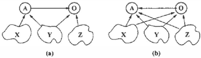
The basic arc reversal operation is relatively straightfor­ ward. Consider a network where variable A is a parent of 0. The variables belonging to the set II(A) U II(O) can be divided into three classes: X = IT(A) \ II(O), Y = IT(A) n II(O), and Z = II(O) \ IT(A) \ {A} (see Fig­ ure l(a)). Suppose we wish to reverse the arc between A and 0. To ensure that the resulting network makes correct independence assertions, we must add parents to both nodes A and 0: in particular, each element of X becomes a par­ ent of 0, and each element of Z becomes a parent of A. A and 0 retain their original parents as well (apart from the re­ versal of the arc between them). The structure of resulting network is illustrated in Figure l(b). We use the notations IIold(A) and IInew(A) to refer to A's parents before and after reversal, respectively (similarly for 0).

The expressions for the new CPT entries are [16):

Note that each term in Equation 1 is in an original CPT, as are the terms in the numerator of Equation 2, while the de­ nominator is simply an entry in the new CPT for 0.

3.2 Arc Reversal with Structured CPTs

Arc reversal often significantly increases the number of par­ ents of the nodes A and 0 involved. Since CPT size in­ creases exponentially with the number of parents, the result­ ing CPTs can become very large and require a prohibitive

amount of computation to construct. However, should the CPTs in the original network exhibit structural regularities, one would expect the new CPTs to do the same. The key to preserving structure during arc reversal is to be able to iden­ tify, using only the structure of the original CPTs, the regu­ larities in the new CPT. The net result is a smaller structured CPT for the nodes involved in the reversal, as well as the benefit of the computational savings associated with com­ puting fewer (distinct) CPT entries. In addition, inference algorithms that exploit CSI can be used after reversal if we are able to retain this structure.1

We now describe a simple tree-structured arc reversal (TSAR) algorithm for constructing tree-structured CPTs for nodes involved in arc reversal assuming tree-structured CPTs for the original network.

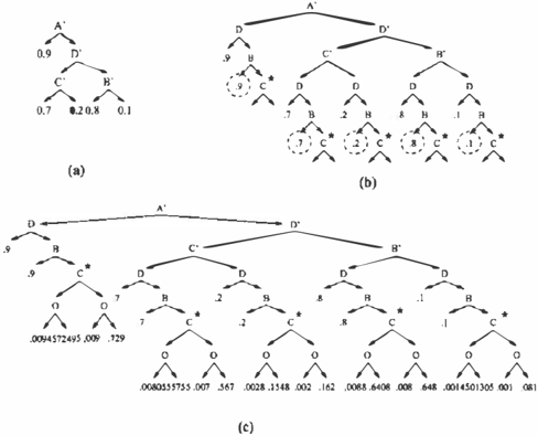
We use the network shown in Figure 2 to illustrate the ba­ sic intuitions underlying TSAR.2 We consider the reversal of the arc between A and 0, where the tree-structured CPTs for both variables are shown in the figure. For ease of ex­ position, all variables in the example are boolean.

When reversing the arc from A to 0, we have IInew(A) = {A', B', C', D', B, C, D, 0} and IInew(O) = {B, C, D, A', B', C', D'}, as indicated in Fig­ ure 3. Had the CPTs for this network been represented in an unstructured form, standard arc reversal would produce a new CPT for A with 2 8 = 256 entries and a new CPT for 0 with 2 7 = 128 entries, and would have required a pro­ portional amount of computation. However, it is clear that since many of the original CPT entries for the nodes A and 0 are identical for different assignments to their parents, the new CPTs must also have many redundancies.

Consider first the new CPT for 0. The following local CSI relations hold between 0 and its new parents:3

1 We expect these ideas to be applicable to compact CPT rep­ resentations apart from trees.

2This network represents a "slice" of a DPN (see next section). 3 We use sets X, Y, Z as in Figure 1; in this example, X = {A', B', C', D'}, Y = 0, and Z = {B, C, D}.

• Let y', z ' be some instantiation of O's original parents (i.e., Y' � Y, Z' � Z), such that 0 is independent of A given y1, z ' . Then for any instantiation x, y, z ofO's new parents consistent withy', z ' , we have (by Equation l) that P ( O j x , Y1 z ) = P(Ojy', z ' ) . For ex­ ample, 0 is independent of A given d (see Figure 2), so P(Oid) remains unchanged for any assignment to IInew(O).
• Let V be some variable in X = IT(A) \ II(O). If, for some instantiation x ' , y ' of a subset of A's original parents (i.e., X' � X, Y � Y), A is independent of V, then for any instantiation of a similar subset of O's new parents of the form x ' 1 y', z, 0 is independent of V. For example, the original tree for A indicates that A and D' are independent given a ' . Since D' is not an original parent ofO, the probability ofO given its new parents cannot vary with D' given a ' .
• Let V be some variable in Z = II( 0) \ II(A) \ {A} such that, for some instantiation y' 1 z ' of a subset of O's original parents (i.e., Y' � Y, Z' � Z), 0 is independent of V given y' 1 z ' , a; for all values a; of A. Then for any instantiationof a similar subset ofO's new parents of the form x, y', z ' , 0 remains indepen­ dent ofV.

These three observations give rise to a simple algorithm for construction a CPT-tree for 0 given its new parents, where an arc from A to 0 is being reversed. The algorithm pro­ ceeds as follows:

1. C re at e a copy of Treeatd(O), re mo v i n g any subtrees that lie below a node labeled A, resulting in ( t h e initial component of) Treenew( 0). For each A-node (say A1) in the tree, record the subtrees associated with each value a E val( A); we de­ note these trees by Treei (a).

1. For each A-node in Treenew(O) (which must be a leaf), Graft a copy of Tree0td( A) onto this location. Reduce the copy of Treeotd(A) by deleting any redundant nodes. We denote by Tree1 (A) the copy of Treeotd( A) added to location A 1. We also mark the root of Tree1 (A).
2. For eachA1: (a)Mergethe trees{Tree1(a): a E va/(A)}1recording the values P( O l a ) for each a E val( A) at the leaves; denote the result by Tree1(0IA). (b) Graft a copy of Tree1 (OIA) to each leaf of Tree1 (A). (c) For each copy so added, compute the value of Equa· lion I using the terms P( Ola) recorded at the leaves of Tree1( 0IA) and the P(a) terms recorded at the leaf of Tree1(A) to which the copy was grafted.

We elaborate on the details by referring to the running ex­ ample. Step 1 requires � hat we duplicate all of Tree old( 0) except for subtrees that he under any node labeled with vari­ able A. This is shown in Figure 4(a), where the asterisk de· notes the location where the removal of the A subtrees oc­ curred (these are recorded below). Any complete branch of that remains denotes a context in which 0 is independent of A, and thus independent of all other new parents: the probability at the leaf node is unchanged. In Figure 4(a), we se :_ that no com � utation is needed to determine P ( 0 I d), P(Oidbc) or P(Oidbc) in the new CPT.

Step 2 involves the replacement of any subtree whose root is labeled with variable A by Tree old( A). This is necessary be­ cause Pnew(O) depends on the probability of A given its old parents. This is illustrated in Figure 4(b) where Treeold(A) is "grafted" to Tree0Id(O) where node A was located.4 At each of the leaf nodes(circled in the example), we now have P(1) given its old parents recorded. While not applica­ ble m our example, Step 2 performs tree reduction as well removing any redundant nodes that may have been added : If, for example, D were a parent of A, all occurrences of D would be removed from Treeotd(A) before grafting, since the value of D is fixed to d earlier in the tree (from Treeotd( 0) ) . Any node labeled D would be replaced by the appropriated subtree. This can play a substantial role if A and 0 share parents (they share none in our example). Fi­ nally, the diagram shows that the root of this grafted tree is marked with an asterisk. This notes the fact that P(O) at

41n general, this takes place at every occurrence of node A.

the leaves of this subtree may in fact be different from their values in Tree old( 0), while any leaf that does not lie below a marked node is such that P(O) is identical to its value in Treeotd(O). Such marks are used below in the construction of Treenew(A), as described later.

Step 3 of the algorithm requires that the subtrees cor­ responding to each value of A that were removed from Tree o ld(O ) at that point now be grafted onto each leaf of Treeotd ( A) that was just added. More precisely, for each such node A that was replaced in Treeold(O), we merge each of its subtrees.5 The leaves of this merged tree dictate P(Oia) for each a E val( A) (given the other relevant par­ ents). The merged tree is then grafted onto the leaves of the relevant copy of Tree old ( A). At the leaf of any "copy" of the meq�ed tree, we compute the value of Equation I, with the reqmred terms readily available. Figure 4(c) illustrates this process. For the (single) copy of Tree0Jd(A) that has been added, we merge the subtrees a and a subtrees that were re­ moved from Treeold(O) at that point: since the a subtree is empty, the merged tree is simply the a subtree. We record both P(Oia) and P(Oia) at each leaf node of the merged tree. This tree is then copied to each of the five leaf nodes wher � P (a) is recorded; and the required conditioning com­ putatiOn takes place for each resulting leaf node.

The CSI reflected in the resulting Treenew(O) is sound:

Theorem 1 Let c be some context determined by a branch ofTreenew( 0) instantiating variables C � llnew( 0). Then 0 is contextually independent ofllnew( 0) \ C given c.

The computational and space savings can be considerable when constructing the new CPT for 0 in tree form. As men­ tioned, the use of tabular CPTs would produce a new CPT for 0 with 128 entries and require 128 calculations of Equa­ tion l . In this example, much of the tree structure of the original CPTs is preserved in Tree new ( 0): it requires only 1.3 disti�ct CPT entries and only 10 calculations of Equa­ tiOn I (smce 3 of the entries are retained from Treevtd(O)).

W,e now �m our atte . ntion to _the construction ofTreenew(A) v1a EquatiOn 2. Agam, certam CSI relations hold:

• Let x ' , y', z' be some partial instantiation of O's new parents (i.e., X' � X, Y' � Y, Z' � Z), such that 0 is independent of its remaining new parents given x ' , y', z', and A is independent of its remaining orig­ inal parents (i.e., those in XU Y) given x ' , y'. Then A is independent of its remaining new parents given x ' , y ' , z' and 0 (by Equation 2). In our example, A is independent of its other parents given a ' while 0 is independent of(other) new parents given dba' c. Thus, A is independent of B', C' and D' given db a' c and 0.
• Let x ' , y', z' be some partial instantiation of O's new parents such thatP(O[x',y'�z') = P(Oiy',z'); that

5 Merging simply requires creating a tree whose branches make the distinction contained in each subtree. We do this by ordering the trees, and grafting each tree in order onto the leaves of the tree resulting fr . om merging its predecessor, removing redundant nodes as appropnate.

is, 0 is independent of A given y1, z1· Then, by Equa­ tion 2, P(Aix', y', z', 0) = P(Aix1, y')Fo r ex­ ample, d renders 0 independ�nt of its parents in both Treeotd(O) and Treenew(O); in particular, 0 is indepen­ dent of A. Thus, any instantiation of A's old parents that fixes P(A) (e.g., a') determines P(A) given its new parents. In our example P(Aia1d) = P(Aia1) and A is independent of other new parents given a1 d.

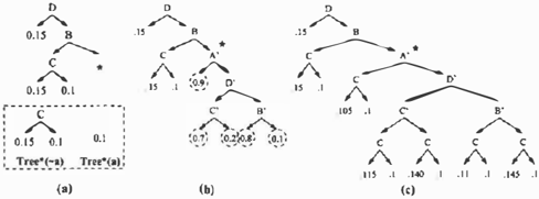
These two observations give rise to a simple algorithm for constructing a CPT-tree for A given its new parents, where an arc from A to 0 is being reversed.

1. Create a copy of Tree0ld(A).
2. For each leaf l of Tree0td(A): to the leaf, and reduce the tree by removing redundant nodes (record the distribution P1 (A)
3. (a) Graft a copy of Treenew(O) labeling the leaf l).
4. (b) Collapse any subtree of the reduced Treenew( 0) which is not marked as altered into a single leaf node; denote this reduced, collapsed tree Tree1(0).
5. (c) Label each unmarked leaf of Tree1(0) with P1(A).
6. (d) Add a node 0 to each leaf lo in the marked subtrees of Tree1 ( 0) (and record the distribution Pto( 0) labeling leaf lo).
7. (e) For each new leaf under the 0-nodes, compute the value of Equation 2 using the terms P1 (A), P1o( 0), and the values P(OIIIotd(O)) determined from Tree0td(O).

We elaborate on the details by referring to the running ex­ ample. Step I requires that we duplicate all of Treeotd(A) and keep track of the distribution labeling each leaf. This is shown in Figure 5(a). Step 2 involves a number of substeps. First, a copy of Treenew(O) is grafted to each leaf of Treeold(A) and reduced as shown in Figure S(b). It also shows how the left subtree under each B node is col­ lapsed by removal of the C node (the circled leaves), and how each "unmarked" leaf inherits P(A) from Treeold(A): since P(O) is identical at unmarked leaves given Ilnew(O) or Ilotd(O), these terms in Equation 2 cancel (thus P(A) need not be computed). Finally, Figure 5(c) shows the ad­ dition of the node for new parent 0 at marked leaf, and the values of P(A) computed according to Equation 2.

Again, the resulting Treenew(A) is sound:

Theorem 2 Let c be a context determined by a branch of Treenew(A) instantiating variables C � I1new(A). Then A is contextually independent ofi1new(A) \ C given c.

Once again we note that this algorithm preserves a consid­ erable amount of structure in this example. Using unstruc­ tured CPTs, the new CPT for A would require 2 8 = 256 entries and the same number of evaluations of Equation 2. Exploitation of tree-structured CPTs allows the new CPT for A to be expressed with only 30 distinct entries, and re­ quires that Equation 2 be evaluated only 20 times (i.e., at the leaves of marked subtrees).6

4 TSAR in the Simulation of DPNs

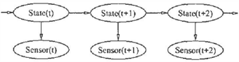
Dynamic probabilistic networks (DPNs) are a particular form of BN used to model temporally-extended systems [5, 11, 10]. Intuitively, we imagine a number of state vari­ ables whose values vary over time, allowing the network to be organized in "slices" consisting of a set of variables at a particular point in time. The system dynamics are often taken to be Markovian and stationary: the causal influences for any variable at timet must be drawn from the set of vari­ ables at time t -1 or time t, and this relation holds for all times t. Thus the DPN can be represented schematically in a very compact fashion by simply representing the relation between two consecutive generic slices at time t and t + 1 (together with priors for root nodes at time 1 ) .

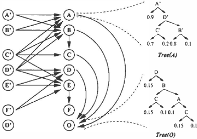
DPNs can be used to model dynamical systems generally, and specifically can be applied to time series models [ 11 ], control problems such as robot or vehicle monitoring and control [12, 10], planning [5] and sequential decision prob­ lems [ 18, 1]. We often distinguish certain variables within a particular slice as state variables, and others as sensor vari­ ables. It is generally only sensor variables that are observ­ able and provide evidence of the system's trajectory. This is illustrated schematically in Figure 6 (following [ 1 0]). We note that the set of state and sensor variables need not be dis­ joint, and that state variables could include decision v a r i ­ ables whose values are set by the controller (possibly de­ pending on the values of previous state variables). Figure 2 (used earlier) illustrates a DPN with a number of state vari­ ables (A through F) and a single sensor variable (0). Our convention is that node A1 denotes variable At (A at time t) and node A denotes At+l·

6We note that these 30 entries are, in fact, not all distinct. But the tree-representation imposes certain redundancies that could be overcome using other function representations.

A common task in DPNs is projection or forecasting, that is, determining, at time t, the distribution over some subset of future variables (i.e., state variables at times later than t) given a set of observations at some points in the past (i.e., evidence at sensor variables at certain points prior to timet). For example, one might want to compute the expected value of a particular policy for some k steps into the future given observations of past behavior of the system. Because of the size ofDPNs, exact solutionofaDPN is impractical inmost settings. Therefore simulation models are often preferred. However, traditional methods such as likelihood weighting [17, 7] will be extremely unsuitable in DPNs exhibiting the schematic structure of Figure 6. Because they are sinks in the network, the sensor variables (which provide the only evidence) are unable to influence the course of the simula­ tion. As demonstrated convincingly by Kanazawa, Koller and Russell [ 1 0], straightforward simulation will often "get off track" very quickly, leading to trials with negligible (or zero) weight. They suggest the use of (partial) evidence in­ tegration in order to keep the simulation close to reality. In­ tuitively, arcs from state variables to sensors within timet are reversed so that observed evidence will strongly influ­ ence the sampled state at timet. The reversal is only partial, however, since sensor variables in the reversed network will generally have as parents state variables from slice t 1. 7

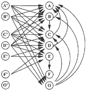
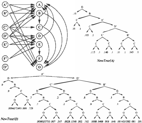
Unfortunately, evidence integration can be expensive. In­ deed, Fung and Chang [7] suggest that, while evidence integration can help convergence of simulation methods tremendously, the computational cost of arc reversal may prove to be a practical obstacle to its applicability. Fortu­ nately, in DPNs, evidence integration benefits from the uni­ form nature of the network: the reversal needs to be com­ puted at one slice only, and can then be applied across all slices. Thus, one substantial burden is overcome. Yet com­ plete "within slice" integration of sensor variables can still be rather costly. Consider the network in Figure 2. Com­ plete reversal of arcs into sensor variable 0 (within a sin­ gle slice only) results in the extremely connected network illustrated in Figure 7. Variables A, B, C, D and 0 have CPTs of sizes 256, 128, 64, 128 and 64, respectively. Fur­ thermore, 0 (which is involved in four reversals) has inter­ mediate CPTs of sizes 128,64 and 32. Arc reversal requires explicit computation of each of these 864 entries. In larger networks, with tens or hundreds of state variables, this can prove a major impediment to evidence integration.

7We take as accepted the crucial role of evidence integration in the convergence of simulation involving DPNs. Our experi­ ments with networks of this type (both with tree-structured CPTs and without) confirm this impression.

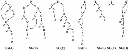
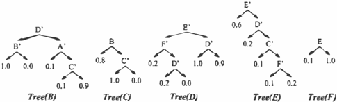
This suggests that tree-structured arc reversal can play an important role in the simulation of DPNs. The computa­ tional burden of evidence integration as well as the size of the resulting CPTs can be considerably lessened by the use of TSAR. For instance, if the CPTs of the remaining nodes in our example DPN are as shown in Figure 8, the sizes of the trees in the reversed network for A, B, C, D and 0 are 30, 33, 23, 72 and 36, respectively, while O's intermediate trees have sizes 13, 11 and 15. Of the total 233 CPT en­ tries represented, only 210 required explicit computation. Our experiments with other similar DPNs suggest that this savings is commonplace. This seems especially true in the evaluation of policies, where actions or decisions play a predominant role. As argued in [3], the representation of action effects often admits a considerable amount ofCSL

Apart from the potential savings it provides during network restructuring, another advantage offered by TSAR is the ability to determine irrelevant variables dynamically. Irrel­ evance can be viewed at the network level. For instance, in the DPN above, we may be interested in the distribution of variable A1· Given such a specific query, a simulation trial need not sample F1 _1 since this cannot impact A1· The ir­ relevance of F1 _ 1 to A1 is dictated by the structure of the DPN. Indeed, Fung and Chang [7] propose irrelevance of this type as a means of speeding simulation, though the � caution that the overhead involved may offset any savings.

8See also (14] for a discussion of this type of relevance.

We focus on a specific problem: assume a DPN has been given and that a certain subset of state variables has been designated as immediately relevant. The simulation is de­ signed to sample these variables over time; the fact that other variables are being sampled is subsidiary to this aim.9 In our example, imagine that A is the variable of interest. What we wish to determine is the set of variables that must be sampled in each slice to ensure we can accurately deter­ mine the conditional probability of A at any future time.

We would hope that "schematic" detection of irrelevance could alleviate overhead difficulties (i.e., the detection of ir­ relevance by processing a single slice in a manner that ap­ plies across all time points). But, clearly, if we need to sam­ ple A at each slice, we cannot ignore F: while Ft-1 doesn't impact At, it does influence At+l through its impact on Dt. The influence of certain variables often "bleeds through" to many or all other variables over time, making network­ level irrelevance unhelpful. Fortunately, the tree-structured CPTs suggest that some variables may be irrelevant to oth­ ers under certain conditions, even if they are not irrelevant at all times. So, while Ft-t might be required in order to sample Dt (which itself impacts At+t, the variable of inter­ est), the tree forD shows that Ft-l has no impact if Et-t is true. This suggests that one should sample E at a particular time slice first; and if it E turns out to be true, one should not sample F at that slice. Some care is required of course, since F may influence other variables of relevance through a different causal chain.

Our goal is a simple algorithm for constructing a condi­ tional sample schedule for the variables within a time slice in which a variable is not sampled if it provably has no influ­ ence on any variable of interest at any future point in time. An example of constraints on such sample schedule might be: "Generate values forE, D, C before F. If e d or edc, do not sample F." Our algorithm proceeds in four phases.

We first identify (unconditionally) relevant variables, those variables that can influence the future value of some vari­ able of interest; in our example, all variables are relevant since all influence A (the variable of interest) over time. This can easily be detected using the topological structure of the network. For our purposes, we now treat the set of unconditionally relevant variables as potentially relevant to the future values of immediately relevant variables.

Second, we construct a sample graph for each relevant variable. This structure describes the dependence of each variable on other variables within the same or previous slice. Essentially, these are directed acyclic graphs gener­ ated from the CPTs for the variables in question, and are similar to binary decision diagrams (BDDs) [4]. The sam­ ple graphs for the seven variables are shown in Figure 9. For example, the graph for variable 0 dictates that, in order to sample it: we need the value of E'; ife', we need F, oth­ erwise we proceed to D; once we sample F (if necessary)

9 For instance, in policy evaluation, one may wish simply to sample and sum value nodes at each slice, with no "direct" interest in other state variables being expressed.

A'

0

we proceed to D and so on.10

The key third phase of the algorithm requires that we de­ termine the conditions under which a (unconditionally rel­ evant) variable is conditionally irrelevant. To begin, we order variables so that the variables first in the ordering have sample graphs (or CPTs) that depend only on previ­ ous variables, and that variables later in the ordering de­ pend only on variables in the same time slice that lie ear­ lier in this ordering. (A suitable ordering for this example is 0, D, B, E, F, C, A.) Then for each variable, we deter­ mine the conditions under which it is required by uncondi­ tionally relevant variables in the next slice (i.e., when must it be known in order to determine the distribution for that variable). Using the ordering of variables suggested, we ap­ ply the variable in question to each sample graph, determin­ ing the set of minimal initial segments of paths (or contexts) in the graph that have no completion leading to the variable in question.

To illustrate, we consider the conditions under which the value ofF at one slice is not required to accurately sam­ ple other variables at the next (or any future) time slice. We apply F to each sample graph, in turn, using our variable ordering. applying F to the graph for 0, we see that con­ ditione is the only one that guarantees F's value is not re­ quired to sample 0. If we apply F to the graph forD, we see again that e is the only such condition. If we then pro­ cess the graph forB, we see that F does not occur, but B depends on the current value of D; since we have already processed D's graph, at that point we can insert the dis­ covered condition for D (i.e., e) at that point in our search through B's graph (thus, the ordering of variables plays an important role). Note that if several distinct paths bypass F, the condition generated is disjunctive: in applying F toE' sample graph, we see that F is irrelevant toE if e VedVedc. We note that F is irrelevant when e for all other variables. 11

10Intuitively, such a graph can be constructed by joining com­ mon subtrees (ignoring leaf values) in the CPT, and collapsing true/false branches from a variables that lead to similar subtrees. This graph can easily be built while the tree is being constructed during arc reversal (if the node is part of a reversed arc). The com­ plexity of identifying common subtrees should not be a limiting factor in this setting. But we should point out that the ideas below can be applied using the trees themselves. Collapsing trees into graphs simply aids the process somewhat.

11 We note that finding all paths and other operations on sam-

Once we have determined the conditions under which F is irrelevant for all variables, their conjunction fixes the con­ ditions under which F is not needed to determine any value at the next slice: in this case, we obtain ed V edc. We note that variables other than F in our example can be ignored under any conditions.

The conditions so obtained for F suggest that one should sample variables within any given slice such that F is sam­ pled after E, D and C, and only when e or edc obtains. Of course, the conditions obtained for other variables might impose other contraints on the ordering. Phase 4 of the al­ gorithm involves construction of a sample schedule that sat­ isfies as many constraints as possible. In this example, since no other variables are irrelevant under any conditions, we simply use this schedule. One could imagine, however, that one might want to sample F before E because of their im­ pact on a third variable. In such a case one could not satisfY both the requirement to sample F before E and the require­ ment to sample E before F. In this case, an arbitrary choice could be made, or some heuristic could be used (e.g., if we had some estimate of the steady state probabilities that sug­ gested e was unlikely, we would know that skipping F was also unlikely, in which case, we might decide to opt for con­ ditionally sampling E based on F rather than vice versa).

Our running example was not designed to ensure a lot of conditional irrelevance, but it does offer the ability to not sample one variable (in each slice) under some conditions. For instance, a simple experiment using A as the inunedi­ ately relevant variable shows that F needs to be sampled in only about a third of the slices: using 20 randomly gener­ ated observation sets (of20 observations each) for our net­ work stretched over 100 time slices, we saw that F was sampled an average of 35 times out of the possible 100 times per run (the results were averaged over 1000 runs per evidence set). While not a large savings in this case (it is only one variable), the savings is proportional to the hori­ zon of interest. For larger networks with substantial hori­ zons, one might generally expect considerable savings from irrelevance processing. The longer the horizon, the less sig­ nificant is the overhead involved in the (single slice) pro­ cessing required. Furthermore, we expect that in large net­ works, a f ew key contexts (rather than variables) may shield variables of interest from large parts of the network.

5 Concluding Remarks

We have described an algorithm for tree-structured arc re­ versal and demonstrated its potential significance for the simulation of DPNs. Advantages include the reduction in (space and computational) overhead for reversal, and the pie graphs can use some of the efficient procedures designed for BDD manipulation [4). Furthennore, this process can be tenni­ nated early if we ever find that the irrelevant condition for a vari­ able with respect to any graph is false, or if the conjunction of con­ ditions f or any (incremental) subset of the graphs is inconsistent: the variable must then be sampled no matter what . For instance, when processing variable E (or D, A, C) on the graph for 0, we see that it must always be sampled, in which case application to other graphs is pointless.

ability to exploit the structured nature of the resulting re­ versed DPNs, especially in dynamic irrelevance detection. There are a number of questions that remain to be ad­ dressed. These include validation of the potential gains of ­ fered by TSAR and its use in simulation in realistic net­ works, and the application of these ideas to other forms of structured BNs. The existence of benchmark DPNs would aid this study. We are also investigating the potential of these ideas in the evaluation of policies for Markov deci­ sion processes.

Acknowledgements: This research was supported by NSERC Research Grant OGP0121843.

References

• [ 1 ] C. Boutilier, R. Dearden, and M. Goldszmidt. Exploiting structure in policy construction. IJCAI-95, pp. 1 1 04--1 1 1 1 , Montreal.
• C. Boutilier, N. Friedman, M. Goldszmidt, and D. Koller. Context-specific independence in Bayesian networks. UAI96, pp. l 1 5-1 23, Portland, OR.
• C. Boutilier and M. Goldszmidt . The frame problem and Bayesian network action representations. Proc. lith Cana­ dian Con f on AI, pp . 6 9-8 3 , Toronto, 1 996.
• [4) R. E. Bryant. Graph-based algorithms for boolean function manipulation. IEEE Trans. Comp., C-35(8):677-69 1 , 1 986.
• [5) T. Dean and K. Kanazawa. A model f or reasoning about per­ sistence and causation. Comp. Intel., 5(3 ): 1 42-1 50, 1 9 89.
• N. Friedman and M. Goldszmidt. Learning Bayesian net­ works with local structure. UAI-96, p p . 2 5 2-2 6 2 , Portland, OR.
• R. Fung and K. Chang. Weighing and integrating evidence f or stochastic simulation in bayesian networks. UAI-89, pp.209-21 9, Windsor.
• D. Geiger and D. Heckennan. Advances in probabilistic rea­ soning. UAI-91, pp. l 1 8-1 26, Los Angeles.
• [9) S. Glesner and D. Koller . Constructing flexible dynamic be­ lief networks from first-order probabilistic knowledge bases. ECSQARU '95, pp.2 1 7-226.
• [I 0] K. Kanazawa, D. Koller, and S. Russell. Stochastic simula­ tion algorithms for dynamic probabilistic networks. IJCAI95, pp.346-35 1 , Montreal.
• [ I I) U. Kjaerulff. A computational scheme for reasoning in dy­ namic probabilistic networks. UAI-92, pp. l 2 1-1 29, Stan­ ford.
• [ 1 2] A. E. Nicholson and J. M. Brady. Sensor validation using dynamic belief networks. UAI-92, pp.207-2 14, Stanf ord.
• [ 1 3] J. Pearl. Probabilistic Reasoning in Intelligent Systems: Net­ works o f Plausible I n f erence. Morgan Kaufmann, 1 988.
• [ 1 4 ) K. Poh and E. Horvitz. A graph-theoretic analysis of inf or­ mation value. UAI-96, pp.427-435, Portland, OR.
• [ I S] D. Poole. Probabilistic Hom abduction and Bayesian net­ works. Artif. Intel., 64( 1 ):8 1-1 29, 1 993.
• [ 1 6) R. D. Shachter . Evaluating influence diagrams. Op. Res., 33(6):871-882, 1986.
• [ 1 7) R. D. Shachter and M. A. Peot. Simulation approaches to general probabilistic inf erence in belief networks. UAI-89, pp.22 1-23 1 , Windsor .
• [ 1 8] J. A. Tatman and R. D. Shachter. Dynamic programming and influence diagrams. IEEE Trans. Sys .. Man and C yber., 20(2):365--379, 1 990.