Systematic vs. Non-systematic Algorithms for Solving the MPE Task

Radu Marinescu

Kalev Kask

School ofinformation and Computer Science University of Califomia, Irvine, CA 92697-3425 { radum,kkask,dechter }@ics. uci.edu

Abstract

The paper explores the power of two system­ atic Branch and Bound search algorithms that exploit partition-based heuristics, BBBT (a new algorithm for which the heuristic information is constructed during search and allows dy­ namic variable/value ordering) and its predeces­ sor BBMB (for which the heuristic information is pre-compiled) and compares them against a number of popular local search algorithms for the MPE problem as well as against the recently pop­ ular iterative belief propagation algorithms. We show empirically that the new Branch and Bound algorithm, BBBT demonstrates tremendous prun­ ing of the search space far beyond its predecessor, BBMB which translates to impressive time sav­ ing for some classes of problems. Second, when viewed as approximation schemes, BBBT/BBMB together are highly competitive with the best known SLS algorithms and are superior, espe­ cially when the domain sizes increase beyond 2. The results also show that the class of belief prop­ agation algorithms can outperform SLS, but they are quite inferior to BBMBIBBBT. As far as we know, BBBT/BBMB are currently among the best performing algorithms for solving the MPE task.

1 INTRODUCTION

The paper presents an extensive empirical study of highly competitive approaches for solving the Most Probable Ex­ planation (MPE) task in Bayesian networks introduced in recent years. We compare two Branch-and-Bound (BnB) al­ gorithms that exploit bounded inference for heuristic guid­ ance on the one hand, against incomplete approximation algorithms, such as stochastic local search, which have proven to be powerful for solving constraint satisfaction (CSP) and boolean satisfiability (SAT) problems in recent years, on the other. We also compare against the class of generalized iterative belief propagation adapted for the

MPE task.

Our Branch-and-Bound algorithms are based on par­ titioning based approximation of inference, called mini-bucket elimination (MBE( i)) first introduced in [Dechter and Rish 1997]). The mini-bucket scheme approximates variable elimination algorithms. Rather than computing and recording functions on many vari­ ables, as is often required by variable elimination, the mini-bucket scheme partitions function computations into subsets of bounded number of variables, i, (the so called i-bound), and records several smaller functions instead. It can be shown that it outputs an upper bound (resp., lower bound) on the desired optimal value for a maximization (resp., minimization) task. This is a flexible scheme that can tradeoff complexity for accuracy; as the i-bound increases both the computational complexity (which is exp( i)) and the accuracy increase (for details see [Dechter and Rish 1997, Dechter and Rish 2003]).

It was subsequently shown in [Kask and Dechter 2001] that the functions generated by MBE( i) can be used to create heuristic functions that guide search. These heuristics have varying strengths depending on the mini-bucket's i-bound, allowing a controlled tradeoff between pre-processing (for heuristics generation) and search. The resulting Branch and Bound with Mini-Bucket heuristic BBMB( i), was evaluated extensively for probabilistic and deterministic optimization tasks. Results show that the scheme overcomes partially the memory explosion of bucket-elimination allowing a gradual tradeoff of space for time, and of time for accuracy.

More recently a new algorithm called BBBT(i) [Dechter et a/. 200 I] was introduced that takes the idea of partition-based heuristics one step further. It explores the feasibility of generating partition-based heuristics during search, rather than in a pre-processing manner. This allows dynamic variable ordering · a feature that can have tremen­ dous effect on search. The dynamic generation of these heuristics is facilitated by a recent extension of mini-bucket elimination to mini-bucket tree elimination (MBTE), a partition-based approximation defined over cluster-trees

Rina Dechter

described in [Dechter et a/.2001]. MBTE outputs multiple (lower or upper) bounds for each possible variable and value extension at once, which is much faster than running MBE n times, one for each variable, to generate the same result

This yields algorithm BBBT(i) that applies the MBTE(i) heuristic computation at each node of the search tree. Clearly, the algorithm has a much higher time overhead compared with BBMB(i) for the same i-bound, but it can prune the search space much more effectively, hope­ fully yielding overall superior performance for some classes of hard problems. Preliminary tests of the algorithms for the MAX-CSP (finding an assignment to a constraint problem that satisfies a maximum number of constraints) task showed that on a class of hard enough problems BBBT( i) with the smallest i-bound ( i=2) is cost-effective [Dechter et a/. 200 1].

Stochastic Local Search (SLS) is a class of incomplete ap­ proximation algorithms which, unlike complete algorithms, are not guaranteed to find an optimal solution, but as shown during the last decade, are often far superior to complete systematic algorithm on CSP and SAT problems. In this paper we wiJI compare a number of best-known SLS algo­ rithms for solving the MPE problem against BBMB/BBBT. Some of these SLS algorithms are applied directly on the Bayesian network, some translate the problem into a weighted SAT problem first and then apply a MAX-wSAT algorithm.

A third class of algorithms are iterative join-graph prop­ agation (IJGP(i)) that applies Pearl's belief propagation algorithm to loopy join-graphs of the belief network [Dechter et a/. 2002].

We experiment with random uniform, Noisy-OR, NxN grid and random coding problems, as well as a number of real world benchmarks. Our results show that 88MB and BBBT do not dominate one another. While BBBT can sometimes significantly improve over 88MB, in many other instances its (quite significant) pruning power does not outweigh its time overhead. Both algorithms are powerful in different cases. In general when large i-bounds are effective 88MB is more powerful, however when space is at issue BBBT with small i-bound is often more powerful. More signif­ icantly, we show that SLS algorithms are overall inferior to BBBT/BBMB, except when the domain size is small. This is unlike what we often see in the case of CSP/SAJ: problems, especially in the context of randomly generated instances. The superiority of BBBT /88MB is especially significant because unlike local search they can prove opti­ mality if given enough time. Finally, we demonstrate that generalized belief propagation IJGP(i) algorithms are often superior to the SLS class as well.

In Section 2 we present background, definitions and de­ scribe relevant recent work on mini-bucket-tree elimina­ tion underlying the BBBT algorithm. Section 3 presents an overview of BBBT, contrasted with 88MB. Section 4 pro­ vides an overview of the SLS algorithms used in our study and the iterative join-graph propagation algorithms. In Sec­ tion 5 we provide our experimental results, while Section 6 concludes.

2 BACKGROUND

2.1 PRELIMINARIES

Belief networks. A belief network is a quadruple BN =< X,D,G,P > (also abbreviated< G,P >) where X= {XI, . . . , Xn} is a set of random variables, D = {D1, ... , Dn} is the set of the corresponding domains, G is a directed acyclic graph over X and P ={PI, ... , Pn}, where P; = P(X;Ipa;) (pa; are the parents of X; in G) denote conditional probability tables (CPTs). Given a function f, we denote by scope(!) the set of arguments of function f. The family of X;, F;, includes X; and its parent variables.

The most common automated reasoning tasks in Bayesian networks are belief updating, most probable explanation (MPE) and maximum aposteriory probability (MAP). In this paper we focus on the MPE task. It appears in applications such as diagnosis, abduction and explanation. For exam­ ple, given data on clinical findings, MPE can postulate on a patient's probable affliction. In decoding, the task is to iden­ tify the most likely input message transmitted over a noisy channel, given the observed output.

DEF!NIT!ON 2.1 (MPE) The most probable explanation problem is to find a most probably complete assign­ ment that is consistent with the evidence, namely, to find an assignment (x�, . . . , x�) such that P(x�, ... , x�) maXx1, · · . ,xn Il�=l P(xk, elxpak )

Singleton-optimality task. In addition to finding the global optimum (MPE), of particular interest to us is the spe­ cial case of finding, for each assignment X; = x;, the highest probability of the complete assignment that agrees with X; = x;. Formally, we want to compute z(X;) = maxx -{Xi} (Il�=l Pk), for each variable X;.

The common exact algorithms for Bayesian inference are join-tree clustering defined over tree-decompositions [Lauritzen and Spiegelhalter 1988] and variable elimination algorithms [Dechter 1999]. The variant we use was pre­ sented recently for constraint problems.

DEFINITION 2.2 (cluster-tree decompositions) [Gottlob et al. l999} Let BN =< X, D, G, P > be a belief network. A cluster-tree decomposition/or BN is a triple D =< T, x, 'ljJ >. where T = (V, E) is a tree, and X and 'ljJ are labeling functions which associate with each vertex v E V two sets, x(v) <::::X and 'lj;(v) <:::: P.

1. For each function P; E P, there is exactly one vertex v E V such thatp; E 'lj;(v), and scope(p;) <:::: x(v).

Procedure CTE

Input:

A Bayesian network EN, a tree-decomposition< T, x, 1/J >.

Output: A set of functions zi as a solution to the singleton-optimality task.

Repeat

1. Select an edge ( u, v) such that m(u, v) has not been computed and u has received messages from all adjacent vertices other than v.
2. ffi(u,v) <---maxeli m (u,v) ITgEc lu st e r (u) ,g;"m(v,u) g (where cluster( u) = 1/J(u) U { m( w, u) I (w, u) E T} ).

Until all messages have been computed.

Return for each i, z(Xi) = maxx(u)-x, [l9Eclus t e r(u) g · such that Xi E cluster(u).

Figure I: Algorithm cluster-tree elimination (CTE) for singleton-optimality task.

1. For each variable Xi E X, the set { v E V[Xi E x( v)} induces a connected subtree ofT. The connect­ edness requirement is also called the running intersec­ tion property.

Let ( u, v) be an edge of a tree-decomposition, the separa­ tor ofu and v is defined as sep(u, v) = x(u) n x(v); the eliminator of u and v is defined as elim( u, v) = x( u) sep(u, v).

DEFINITION 2.3 (tree-width, hyper-width, induced-width) The tree-width of a tree-decomposition is tw maxvEV l x(v) l -1, its hyper-width is hw maxvEV 11/J(v)[, and its maximum separator size is s = max(u,v)EE [sep(u,v)[. The tree-width of a graph is the minimum tree-width over all its tree-decompositions and is identical to the graph's induced-width.

2.2 CLUSTER-TREE ELIMINATION

Algorithm Cluster-Tree Elimination (CTE) provides a uni­ fying space concious description of join-tree clustering al­ gorithms. It is a message-passing scheme that runs on the tree-decomposition, well-known for solving a wide range of automated reasoning problems. We will briefly describe its partition-based mini-clustering approximation that forms the basis for our heuristic generation scheme.

CTE provided in Figure I computes a solution to the sin­ gleton functions zi in a Bayesian network. It works by computing messages that are sent along edges in the tree. Message m(u,v) sent from vertex u to vertex v, can be computed as soon as all incoming messages to u other than m(v,u) have been received. As leaves compute their messages, their adjacent vertices also qualify and com­ putation goes on until all messages have been computed. The set of functions associated with a vertex u augmented with the set of incoming messages is called a cluster, cluster(u) = 1/J (u) U(w,u)ET m(w,u) · A message m(u,v) is computed as the product of all functions in cluster( u) excluding m(v,u) and the subsequent elimination of vari­ ables in the eliminator of u and v. Formally, m(u,v) = maxelim(u,v) ([lg Ec l u ster( u ) , g;"m(v,u) g). The computation is done by enumeration, recording only the output message. The algorithm terminates when all messages are computed.

The functions z(X;) can be computed in any cluster that contains Xi by eliminating all variables other than X; .

It was shown that [Dechter et a/.2001] the complexity of CTE is time O(r · (hw + dg) · d tw +l) and space O(r · d8), where r is the number of vertices in the tree-decomposition, hw is the hyper-width, dg is the maximum degree (i.e., number of adjacent vertices) in the tree, tw is the tree-width, d is the largest domain size and s is the maximum separator size. This assumes that step 2 is computed by enumeration.

There is a variety of ways in which a tree-decomposition can be obtained. We will choose a particular one called bucket-tree decomposition, inspired by viewing the bucket­ elimination algorithm as message passing along a tree [Dechter et a/.2001]. Since bucket-tree is a special case of a cluster-tree, we define the CTE algorithm applied to a bucket-tree to be called Bucket-Tree Elimination (BTE). BTE has time and space complexity O(r . d tw+ l ) .

2.3 MINI-CLUSTER-TREE ELIMINATION

The main drawback of CTE and any variant of join-tree algorithms is that they are time and space exponential in the tree-width (tw) and separator (s) size, respectively [Dechter et al.2001, Mateescu et al.2002], which are often very large. In order to overcome this problem, partition­ based algorithms were introduced. Instead of combining all the functions in a cluster, when computing a message, we first partition the functions in the cluster into a set of mini­ clusters such that each mini-cluster is bounded by a fixed number of variables ( i-bound), and then process them sepa­ rately. The algorithm, called Mini-Cluster-Tree Elimination (MCTE) approximates CTE and it computes upper bounds on values computed by CTE.

In the Mini-Cluster-Tree Elimination the message M(u,v) that node u sends to node v is a set of functions computed as follows. The functions in cluster(u) - M(v,u) are par­ titioned into P = P1, · · ·, Pk, where [scope(Pj)l ::; i, for a given i. The message M(u,v) is defined as M(u,v) = {maxeli m (u , v) [l gE P g[Pj E P}. Algorithm MCTE ap­ plied to the bucket-tr � e is called Mini-Bucket-Tree elimina­ tion (MBTE) [Dechter et a/.2001].

Since the scope size of each mini-cluster is bounded by i, the time and space complexity of MCTE (MBTE) is expo-

Procedure BBBT(T,i,s,L)

Input:

Bucket-tree T, parameter i,set of instantiated variables S = s, lower bound L.

Output:

MPE probability conditioned on s.

1. If S = X, return the probability of the current complete assignment.
2. Run MBTE(i); Let { mzJ} be the set of heuristic values computed by MBTE(i) for each XJ E XS.
3. Prune domains of uninstantiated variables, by removing values x E D(Xr) for which mzr(x):::; L.
4. Backtrack: If D(X1) = 0 for some variable Xr, return 0.
5. Otherwise let XJ be the uninstantiated variable with the smallest domain: XJ = argminxkEx-siD(Xk)l.
6. Repeat while D(XJ) =f0
7. Let Xk be the value of XJ with the largest heuristic estimate: Xk = argmaxx j E D ( X ) ffiZJ(XJ).
8. Set D(X) = D(X) - Xk.
9. Compute mpe = BBBT(T,i,sU {XJ = xk},L).
10. Set L = max(L, mpe).
11. Prune D(XJ) by L.
12. Return£.

Figure 2: Branch-and-Bound with MBTE (BBBT).

nential in i. However, because of the partitioning, the func­ tions ZJ cannot be computed exactly any more. Instead, the output functions of MCTE (MBTE), called mzj, are upper bounds on the exact functions Zj ([Dechter et a/.2001]).

Clearly, increasing i is likely to provide better upper bounds at a higher cost. Therefore, MCTE(i) allows trading upper bound accuracy for time and space complexity.

3 PARTITION-BASED BnB

This section focuses on the two systematic algorithms we used. Both use partition based mini-bucket heuristics.

3.1 BoB WITH DYNAMIC HEURISTICS (BBBT)

Since MBTE( i) computes upper bounds for each singleton­ variable assignment simultaneously, when incorporated within a depth-first Branch-and-Bound algorithm, MBTE(i) can facilitate domain pruning and dynamic variable order­ mg.

Such a Branch-and-Bound algorithm, called BBBT(i), for solving the MPE problem is given in Figure 2. Initially it is called with BBBT( < T, x, 1/J >, i, 0, 0). At all times it maintains a lower bound L which corresponds to the prob­ ability of the best assignment found so far. At each step, it executes MBTE( i) which computes the singleton assign­ ment costs mzi for each uninstantiated variable Xi (step 2), and then uses these costs to prune the domains of uninstan­ tiated variables by comparing L against the heuristic esti­ mate of each value (step 3). If the cost of the value is not more than L, it can be pruned because it is an upper bound. If as a result a domain of a variable becomes empty, then the current partial assignment is guaranteed not to lead to a better assignment and the algorithm can backtrack (step 4). Otherwise, BBBT expands the current assignment picking a variable Xj with the smallest domain (variable ordering in step 5) and recursively solves a set of subproblems, one for each value of XJ, in decreasing order of heuristic estimates of its values (value ordering in step 6). If during the solu­ tion of the subproblem a better new assignment is found, the lower bound L can be updated (step 6iv).

Thus, at each node in the search space, BBBT(i) first exe­ cutes MBTE(i), then prunes domains of all un-instantiated variables, and then recursively solves a set of subproblems. BBBT performs a look-ahead computation that is similar (but not identical) to i-consistency at each search node.

3.2 BnB WITH STATIC MINI-BUCKETS (BBMB)

As described in the introduction, the strength of 88MB( i) was well established in several empirical studies [Kask and Dechter 200 1]. We describe the main differences between BBBT and 88MB:

• BBMB(i) uses as a pre-processing step the Mini­ Bucket-Elimination, which compiles a set of func­ tions that can be used to assemble efficiently heuris­ tic estimates during search. The main overhead is therefore the pre-processing step which is exponen­ tial in the i-bound but does not depend on the num­ ber of search nodes. BBBT( i) on the other hand com­ putes the heuristic estimates solely during search using MBTE( i). Consequently its overhead is exponential in the i-bound multiplied by the number of nodes visited.
• Because of the pre-computation of heuristics, 88MB is limited to static variable ordering, while BBBT uses a dynamic variable ordering.
• Finally, since at each step, BBBT computes heuristic estimates for all un-instantiated variables, it can prune their domains, which provides a form of look-ahead. 88MB on the other hand generates a heuristic esti­ mate only for the next variable in the static ordering and prunes only its domain.

4 NON-SYSTEMATIC ALGORITHMS

This section focuses on two different types of incomplete algorithms: stochastic local search and iterative belief prop­ agation.

4.1 LOCAL SEARCH

Local search is a general optimization technique which can be used alone or as a method for improving solutions found by other approximation scheme. Unlike the Branch-and­ Bound algorithms, these methods do not guarantee an opti­ mal solution. [Park 2002] showed that an MPE problem can be converted to a weighted CNF expression whose MAX­ SAT solution immediately produces the solution of the cor­ responding MPE problem. Subsequently, local search al­ gorithms initially developed for the weighted MAX-SAT domain can be used for approximating the MPE problem in Bayesian networks. We continue the investigation of Guided Local Search (GLS) and Discrete Lagrangian Mul­ tipliers (DLM) algorithms, as well as a previous approach (SLS) proposed in [Kask and Dechter 1999].

The method of Discrete Lagrangian Multipliers [Wah and Shang 1997] is based on an extension of constraint optimization using Lagrange multipliers for con­ tinuous variables. In the weighted MAX-SAT domain, the clauses are the constraints, and the sum of the unsatisfied clauses is the cost function. In addition to the weight we, a Lagrangian multiplier .Ac is associated with each clause. The cost function for DLM is of the form:

where C ranges over the unsatisfied clauses. Every time a local maxima is encountered, the .\s corresponding to the unsatisfied clauses are incremented by a adding a constant. Guided Local Search [Mills and Tsang 2000] is a heuristi­ cally developed method for solving combinatorial optimiza­ tion problems. It has been shown to be extremelly efficient at solving general weighted MAX-SAT problems. Like DLM, GLS associates an additional weight with each clause C (.Ac). The cost function in this case is essentially I: c .Ac, where C ranges over the unsatisfied clauses. Every time a local maxima is reached, the .As of the unsatisfied clauses with maximum utility are increased by adding a constant, where the utility of a clause C is given by we/ ( 1 + .Ac). Unlike DLM, which increments all the weights of the un­ satisfied clauses, GLS modifies only a few of them.

Stochastic Local Search is a local search algorithm that at each step performs either a hill climbing or a stochastic vari­ able change. Periodically, the search is restarted in order to escape local maxima. It was shown to be superior to simu­ lated annealing and some pure greedy search algorithms.

In [Park 2002] it was shown that, among these three al­ gorithms, GLS provided the best overall performance on a variaty of problem classes, both random and real-world benchmarks.

4.2 ITERATIVE JOIN-GRAPH PROPAGATION

The Iterative Join Graph Propagation (IJGP) [Dechter et a/. 2002] algorithm belongs to the class of generalized belief propagation methods, recently pro­ posed to generalize Pearl's belief propagation algorithm [Pearl 1988] using analogy with algorithms in statistical physics. This class of algorithms, developed initially for belief updating, is an iterative approximation method that applies the message passing algorithm of join-tree cluster­ ing to join-graphs, iteratively. It uses a parameter i that bounds the complexity and makes the algorithm anytime. Here, we adapted the IJGP(i) algorithm for solving the MPE problem by replacing the sum-product messages with max-product message propagation.

5 EXPERIMENTAL RESULTS

We tested the performance of our scheme for solving the MPE task on several types of belief networks- random uni­ form and Noisy-OR Bayesian networks, NxN grids, coding networks, CPCS networks and 9 real world networks ob­ tained from the Bayesian Network Repository1· On each problem instance we ran BBBT(i) and BBMB(i) with var­ ious i-bounds, as heuristics generators, as well as the local search algorithms discussed earlier. We also ran the Itera­ tive Join Graph Propagation algorithm (IJGP) on some of these problems.

We treat all algorithms as approximation schemes. Algo­ rithms BBBT and BBMB have any-time behavior and, if allowed to run until completion, will solve the problem ex­ actly. However, in practice, both algorithms may be termi­ nated at a time bound and may return sub-optimal solutions. On the other hand, neither the local search techniques, nor the belief propagation algorithms guarantee an optimal so­ lution, even if given enough time.

To measure performance we used the accuracy ratio opt = Palg I PMPE between the value of the solution found by the test algorithm (Pa19) and the value of the optimal so­ lution (PMPE), whenever PMPE was available. We only report results for the range opt 2: 0.95. We also recorded the average running time for all algorithms, as well as the average number of search tree nodes visited by the Branch­ and-Bound algorithms. When the size and difficulty of the problem did not allow an exact computation, we compared the quality of the solutions produced by the respective algo­ rithms in the given time bound. For each problem class we chose a number of evidence variables, randomly and fixed their values.

1www.cs.huji.ac.il/labs/compbio!Repository

Table 1: Average accuracy and time. Random Bayesian (N=lOO, C=90, P=2). w*=l7, 10 evidence, 100 samples.

K	BBBT B B M B IJGP i=2 %(time]{nodes}	BBBT 88 M B IJGP i=4 %[time]{nodes}	BBBT BBMB IJGP i=6 %[timeJ{nodes}	BBBT 88MB IJGP i=8 o/o[time]{nodes}	BBBT 88MB IJGP i=\0 %[timeJ{nodes}	GLS %[time]	DLM %(time]	SLS %[time]
2	90[6 3o!V9�� 71(2.19]{1.6M} 62(0.041	100[1.19)!78�� 92[0.17](0.1M} 66[0.061	100[0 6�1 , \�66/ 92(0.02]{lOK) 66(0.131	100(0.44))�1;) 86[0.01](3K) 71[0.321	100(0.43��"�! 91[0.01]{1.2K) 67(0.871	100(1.051	0[30.011	0(30.011
3	28[4661,! , 19�1 5[43.1]{16M} 34[0.071	65[275)j;s�1 78[24.4](8.2M) 37(0.181	86[15.4)!,1.1�� 90(3.20({0.8M) 36[0.941	86(19.3 , 1 , � 45 �] , 89[1.23](0.3M) 43(5.381	80[27 5H2BJ , 83[058]{52.5K} 44(32 . 51	39[44.021	0[60.011	0[60.011
4	24(95.�1} , 63K) 3(89.41{47M) 17[0.141	46(74.7J , I}3.41 � ;l 42(85.5](37M} 14(0.471	65(54.1) , 1 , !.6K;J 89(25.4]{8M) 14(4.331	67(65.;1 , 1,44 �] . 90[5.441{I.SM} 17(43.31	37[151.2].1,' � } . 99(4.821{O.JM) 20(468.51	5[114.91	0[120.01]	0(120.011

5.1 RANDOM BAYESIAN NETWORKS AND NOISY-OR NETWORKS

The random Bayesian networks were generated using pa­ ran1eters (N, K, C, P), where N is the nurnber of variables, K is their domain size, C is the number of conditional prob­ ability tables (CPTs) and P is the number of parents in each CPT. The structure of the network is created by ran­ domly picking C variables out of N and, for each, ran­ domly selecting P parents from their preceding variables, relative to some ordering. For random uniform Bayesian networks, each probability table is generated uniformly ran­ domly. For Noisy-OR networks, each probability table rep­ resents an OR-function with a given noise and leak proba­ bilities: P(X = OIY1,. · · , Yp) = Pleak X TIY,=l Pnoise

Tables I and 2 present experiments with random uniform Bayesian networks and Noisy-OR networks, respectively. In each table, parameters N, C and P are fixed, while K, controlling the domain size of the network's variables, is changing. For each value of K, we generate 100 instances. We gave each algorithm a time limit of 30, 60 and 120 sec­ onds, depending on the value of the domain size. Each test case had 10 randomly selected evidence variables. We have highlighted the best performance point in each row.

For example, Table 1 reports the results with random prob­ lems having N=lOO, C=90, P=2. Each horizontal block cor­ responds to a different value of K. The columns show results for BBBT/BBMB/IJGP at various levels of i, as well as for GLS, DLM and SLS. Looking at the first line in Table 1 we see that in the accuracy range opt;::: 0.95 and for the small­ est domain size (K = 2) BBBT with i=2 solved 90% of the instances using 6.30 seconds on average and exploring 3.9K nodes, while BBMB with i=2 only solved 71% of the in­ stances using 2.19 seconds on average and exploring a much larger search space (1.6M nodes). GLS significantly outper­ formed the other local search methods, as also observed in [Park 2002] and solved all instances using 1.05 seconds on average. However, as BBBT(i)'s bound increases, it is bet­ ter than GLS. As the domain size increases, the problem instances become harder. The overall performance of local search algorithms, especially GLS 's performance, deterio­ rates quite rapidly.

When comparing BBBT(i) to BBMB(i) we notice that at

(q)

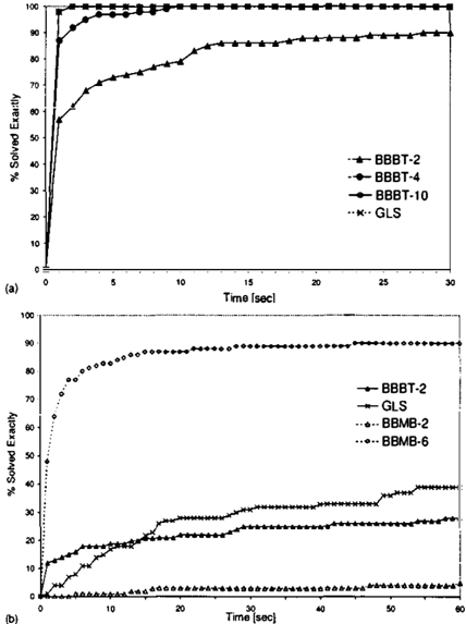
Figure 3: Random Bayesian (N=lOO, C=90, P=2) (a) K=2 (b) K=3. 10 evidence, 100 samples.

larger domain sizes (K E {3, 4}) the superiority of BBBT(i) is more pronounced for small i-bounds (i=2,4), both in terms of the quality of the solution and search space ex­ plored. This may be significant, because small i-bounds require restricted space.

In Figure 3 we provide an alternative view of the perfor­ mance of BBBT(i)/BBMB(i) against GLS as anytime al­ gorithms. Let Falg(t) be the fraction of problems solved completely by the test algorithm al g by time t. Each graph in Figure 3 plots FsBBT(i)(t), FsBMB(i)(t) for some selected values of i, as well as FaLs(t). Two dif­ ferent values of the domain size are discussed, K =2 and K=3, respectively. Figure 3 shows the distributions of FssBT(i)(t), FsBMB(i)(t) and FaLs(t) for the random uniform Bayesian networks when N=lOO, C=90, P=2 (cor­ responding to the first two rows in Table 1 ).

Table 2: Average accuracy and time. Random Noisy-OR (N=IOO, C=90, P=2). Pnoise = 0.2, Pzeak = 0.01. w*=l7, I 0 evidence, I 00 samples.

K	BBBT BBMB IJGP i=2 %[time]	BBBT BBMB IJGP i=4 %[time]	BBBT 88MB IJGP j:6 %(time]	BBBT 88MB IJGP i=8 %(timc]	BBBT 88MB JJGP i=IO %[time]	GLS %[time]	DLM %[time]	SLS %[time]
2	84[7.34] 61[3.49] 62[0.04]	98[2.48] 91[0.30] 66[0.06]	100[0.88] 89[0.05] 66[0.13]	100[0.66] 88[0.02] 71[0.31]	100[0.591 88[0.02] 67[0.86]	100[1.25]	0[30.02]	0[30.02]
3	36[42.2] 8[47.5] 34[0.04]	78[19.1] 77[18.4] 37[0.10]	95[9.64[ 95[1.81] 36[0.49]	94[10.7] 86[0.71] 43[2.86]	93[16.8] 84[0.33] 44[17.0]	49[38.7]	0[60.02]	0[60.01]
4	24[97.7] 2[114.4] 17[0.06]	40[80.3] 39[92.3] 14[0.23]	61[62.4] 84[33.2] 14[2.12]	58[82.0] 90[7.39] 17[21.9]	30[269] 99[7.95[ 20[226.8]	5[115.03]	0[120.01]	0[120.01]

Table 3: #wins given fixed time bound. Random Networks (N=IOO,C=90,P=3). w*=30, 10 evidence, 30 samples.

K	BBBT/GLS BBMB/GLS i 2 #best	BBBT I GLS BBMB /GLS ' 3 #best	BBBT I GLS BBMB/GLS •4 #best	BBBT I GLS BBMB/GLS i 5 #best	BBBT/GLS BBMB/GLS i 6 #best
2	0/29 0/24	0125 0/19	0/23 0/19	0/21 015	0/20 0/5
3	4/26 1/29	5125 2128	5125 2/28	9/21 2/28	10/20 4/26
5	28/2 5125	28/2 5125	3010 7/23 24/6	30/0 12!18	30/0 23/7
		2218		19/11
7	25/5				21/9
		15/15			25/5
	18/12		17/13	20/10

Clearly, if F alg' (t) > F azg; (t), then F alg' (t) completely dominates Fa19; (t). For example, in Figure 3(a), GLS is highly competitive with BBBT( I 0) and both signifi­ cantly outperform BBBT( i)/BBMB( i) for smaller i-bounds. In contrast, Figure 3(b) shows how the best local search method deteriorates as the domain size increases.

We also experimented with a much harder set of random Bayesian networks. The dataset consisted of random net­ works with parameters N=IOO, C=90, P=3. In this case, the induced width of the problem instances was around 30, thus it was not possible to compute exact solutions. We studied four domain sizes KE{2, 3, 5, 7}. For each value of K, we generate 30 problem instances. Each algorithm was allowed a time limit of 30, 60, 120 and 180 seconds, depending on the domain size. We found that the solutions generated by DLM and SLS were several orders of magnitude smaller than those found by GLS, BBBT and BBMB. Hence, we only report the latter three algorithms.

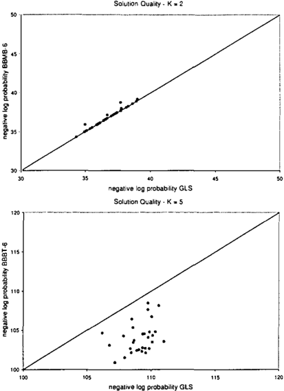
Table 3 compares the frequency that the solution was the best for each of the three algorithms (ties are removed). We notice again that GLS excelled at finding the best solution for smaller domain sizes, in particular for K=2 and 3. On the other hand, at larger domain sizes (KE{ 5,7} ), the power of BBBT( i) is more pronounced for smaller i-bounds, whereas BBMB(i) is more efficient at larger i-bounds. Figure 4 shows, pictorially, the quality of the solutions produced by GLS against the ones produced by BBBT(i)/BBMB(i). For each plot, corresponding to a different value of the do­ main size K, the X axis represents the negative log proba­ bility of the solutions found by GLS and the Y axis repre­ sents the negative log probability of the solutions found by BBBT(i)/BBMB(i). The superiority of BnB-based methods

Table 4: BBBT vs. BBMB. Random networks (N=IOO, C=90, P=3). 10 evidence, 30 samples, 30 seconds.

K	BBBT/BBMB j:2 #wins #nodes	BBBT/BBMB j:3 #wins #nodes	BBBT I BBMB j:4 #wins # n o d es	BBBT/ BBMB i:S #wins #nodes
2	20/10 15.3K/13.8M	12118 14.5K/16.2M	18/12 12.3K/15.9M	18112 9.4K/11.8M
3	27/3 19.9K/16.3M	26/4 13.8K/16.8M	29/1 12.3K/15.9M	28/2 4.8K/14.2
5	291! 18.3KII0.5M	30/0 9.1K/13.8M	30/0 3.5K/13.2M	27/3 0.9K/12.6M
7	24/6 7.7K/8.3M	26/4 3.4K/10.6M	14/16 I14/10.9M	10/20 8/9.6M

for larger domain sizes is significant since these are algo­ rithms that can prove optimality when given enough time, unlike local search methods. Not if the superiority of GLS for KE{2,3} may be a function of the time bound for these hard instances.

Table 4 shows comparatively the performance of BBBT as compared to BBMB. Each entry in the table shows the num­ ber of times BBBT produced a better solution than BBMB (#wins) as well as the average number of search tree nodes visited by both algorithms.

5.2 GRID NETWORKS

In grid networks, N is a square number and each CPT is generated uniformly randomly or as a Noisy-OR function. We experimented with a synthetic set of I 0-by-1 0 grid net­ works. We report results on three different domain sizes.

Table 5: Average accuracy and time. Random Grid Net­ works (N=lOO). w*=l5, 10 evidence, 100 samples.

K	BBBT/ BBMB i=2 %[time]	BBBT! 88MB i=A %[time]	BBBT/ BBMB i=6 %(time]	BBBT/ BBMB i=8 %[time]	BBBT/ BBMB i=lO %[time]	GLS %[time]	DLM %[time]	SLS %[time]
2	5![17.7] 1(29.9]	99[2.62] 13(23.7]	100[0.66] 93(2.16]	100[0.48] 92(0.08]	100 )0. 4 2 ) 95(0.02]	100(1.54]	0(30.01]	0(30.01]
3	3(58.7] 0(60.01]	28[47.4] 1(58.9]	lS0(19.5] 25(50.9]	93(14.8] 89(8.63]	94) 2 3 .2 ) 92(0.73]	4(58.7)	0(60.01]	0[60.01]
4	1]118.8] 0(120]	12(108.3) 0[120]	46(78.4) 6[113.4]	61(88.5] 72(46.4]	33[136) 85[9.91)	0[120)	0(120)	0(120)

Table 6: Average BER and time. Random Coding Networks (N=200, P=4). w*=22, 60 seconds, 100 samples.

"	BBBT 88MB IJGP	BBBT BBMB IJGP	BBBT 88MB IJGP	BBBT BBBT 88MB 88MB IJGP IJGP	IBP GLS SLS
	, ., BER[timc]	·-4 BER[timc)	•=o BER[timc]	,., '•IU BER[timc] BER(time]	BER[time]
0.32	0.0056(3.18) 0.0034[0.07] 0.0034[0.16]	0.0104(2.87) 0.0034(0.08] 0.0034[0.18]	0.0072(1.75] 0.0034(0.03) 0.0034(0.33]	0.0034[0.72] 0.0034(0.59] 0.0034(0.01) 0.0034(0.02) 0.0034(0.92) 0.0034(3.02]	0.0034(0.01) 0.2344(60.01] 0.4980(60.01]
0.40	0.0642(19.4] 0.0114[0.63] 0.0114(0.16)	0.0400[12.8] 0.0114[0.53] 0.0138[0.18]	0.0262[6.96] 0.0114[0.12] 0.0118[0.33]	0.0148[4.52] 0.0190[4.34] 0.01!4[0.05] 0.0114(0.04] 0.0116[0.91] 0.0120[3.02]	0.0108]0.01] 0.2084(60.01] 0.5!28[60.0I]
0.52	0.1920(48.1] 0.0948[1.35] 0.1224[0.08]	o.I790[4Z:OJ 0.0948[1.47] 0.1242[0.09]	0.1384[31.3] 0.0948[0.36] 0.1256(0.16]	0.1144[21.4] 0.1144[19.7] 0.0948[0.11] 0.0948(0.05] 0.1236(0.47] 01132(1.54]	0.0894l0.011 0.2462(60.02] 0.5128[60.01]

For each value of K, we generate l 00 problem instances. Each algorithm was allowed a time limit of 30, 60 and 120 seconds, depending on the domain size. Table 5 shows the average accuracy and running time for each algorithm.

5.3 RANDOM CODING NETWORKS

Our random coding networks fall within the class of linear block codes. They can be represented as four-layer belief networks having K nodes in each layer. The decoding algo­ rithm takes the coding network as input and the observed channel output and computes the MPE assignment. The performance of the decoding algorithm is usually measured by the Bit Error Rate (BER), which is simply the observed fraction of information bit errors.

We tested random coding networks with K=50 input bits and various levels of channel noise 0'. For each value of 0' we generate 100 problem instances. Each algorithm was allowed a time limit of 60 seconds. Table 6 reports the av­ erage Bit Error Rate, as well as the average running time of the algorithms. We see that BBBT/BBMB outperformed considerably GLS. On the other hand, only BBMB is com­ petitive to IBP, which is the best performing algorithm for coding networks.

5.4 REAL WORLD NETWORKS

Our realistic domain contained 9 Bayesian networks from the Bayesian Network Repository, as well as 4 CPCS net­ works derived from the Computer-Based Care Simulation system. For each network, we ran 20 test cases. Each test case had 10 randomly selected evidence variables, ensuring that the probability of evidence was positive. Each algo­ rithm was allowed a 30 second time limit.

Table 7 summarizes the results. For each network, we list the number of variables, the average and maximum domain size for its variables, as well as the induced width. We also provide the percentage of exactly solved problem instances and the average running time for each algorithm.

In terms of accuracy, we notice a significant dominance of the systematic algorithms over the local search meth­ ods, especially for networks with large domains (e.g. Bar­ ley, Mildew, Diabetes, Munin). For networks with rela­ tively small domain sizes (e.g. Pigs, Water, CPCS net­ works) the non-systematic algorithms, in particular GLS, solved almost as many problem instances as the Branch­ and-Bound algorithms. Nevertheless, the running time of BBBT/BBMB was much better in this case, because GLS had to run until exceeding the time limit, even though it might have found the optimal solution within the first fe\v it� erations. BBBT /BBMB on the other hand terminated, hence proving optimality.

We also used for comparison the IJGP algorithm, set up for 30 iterations. In terms of average accuracy, we notice the stable performance of the algorithm in almost all test cases. For networks with large domain sizes, IJGP( i) significantly dominated the local search algorithms and in some cases it even outperformed the BBBT( i)/88MB( i) algorithms (e.g. Barley, Mildew, Munin).

6 CONCLUSION

The paper investigates the performance of two Branch-and­ Bound search algorithms (BBBT/BBMB) against a number of state-of-the-art stochastic local search (SLS) algorithms for the problem of solving the MPE task in Bayesian net­ works. Both BBBT and BBMB use the idea of partioning­ based approximation of inference for heuristic computa­ tion, but in different ways: while BBMB uses a static pre­ computed heuristic function, BBBT computes it dynami­ cally at each step. We observed over a wide range of prob­ lem classes, both random and real-world benchmarks, that BBBT/BBMB are often superior to SLS, except in cases when the domain size is small, in which case they are com­ petitive. This is in stark contrast with the performance of systematic vs. non-systematic on CSP/SAT problems, where SLS algorithms often significantly outperform com­ plete methods. An additional advantage of BBBT/BBMB is that as complete algorithms they can prove optimality if given enough time, unlike SLS.

When designing algorithms to solve an NP-hard task, one cannot hope to develop a single algorithm that would be su­ perior across all problem classes. Our experiments show that BBBT/BBMB, when viewed as a collection of algo­ rithms parametrized by i, show robust performance over a wide range of MPE problem classes, because for each prob­ lem instance there is a value of i, such that the performance of BBBT( i)/88MB( i) dominates that of SLS.

Table 7: Results for experiments on 13 real world networks. Average accuracy and time.

Network	# vars	avg. d om.	m" dom.	w•	BBBT/ 88MB/ lJGP i=2 %[time]	BBBT/ 88MB/ IJGP i=J %[time]	BBBT/ 88MB/ IJGP i=4 %[time]	BBBT/ BBMB/ lJGP i=5 %[time]	BBBT/ 88MB/ JJGP i=6 %[time]	BBBT/ 88MB/ lJGP i=7 %(time]	BBBT/ 88MB/ JJGP j:8 %(time]	BBBT/ 88MB/ UGP i=IO %[time]	GLS % [time]	DLM % [time]	SLS % [time]
Barley	48	8	67 8	67[0.99]		67[1.11]	90[6.33] 25[12.8] 63[1.49]	100[4.28] 40[2.32] 70[5.32l	100[3.29] 65[0.43] 80[17.9]	100[2.81] 90[0.85]	100(2.91) 100(2.41)		0 [30.01]	0 [30.01]	0 [30.01]
Diabetes•	413	II	21 5		0[120] 0[120] 3[8.60]	0[123] 0[120] 3[11.2]	0[127] 5[114] 43[86.0]	9012l.J] 10012.01] 97[311.1]	100[384.6]				0 [120.01]	0 [120.01]	0 [120.01]
Mildew	35	17	100	4	100[0.28] 30[10.5] 90[3.59]	10010.17] 65[7.5] 87[3.68]	100[0.56] 95[0.18] 97[33.3]	100[53.2]					15 [30.02]	0 [30.02]	90 [30.02]
Muninl	189	5	21	II	90[6.13] 0[30] 90[0.45]	90[0.49]	10016.48] 5[27.2] 97[1.10]	93[4.28]	40[23.8] 20[24.1] 93[14.5]	97[70.2]	75[13.4] 70[6.77] 100[191.9]	80[43.1] 100[9.03]	10 [30.02]	0 [30.02]	0 [30.02]
Munin2 1003		5	21	7	95[1.65] 95[30.3] 95[2.44]	95[1.73] 95[31.7] 95[2.94]	95[1.65] 95[30.5] 95[5.17]	95[1.99] 95[31.8] 100[20.3]	95[2.32] 95[31.3] 95[64.9]	95[2.48] 100[30.5]	100]1.971 10011.84]		0 [30.01]	0 [30.01]	0 [30.01]
MuninJ	1044	5	21	7	0[30.8] 0[30.2] 80[1.47]	0[30.9] 0[31] 95[1.72]	0[31.3] 0[32.3] 85[3.10]	5[31.7] 5[29.9] 85[10.8]	0[40.9] 0[32.7] 90[38.9]	90[4.72] 95[2.14]	100]2.2] 10011.01]		0 [30.02]	0 [30.02]	0 [30.02]
Munin4	1041	5	21	8	0[31] 0[30.2] 85[1.52]	0[31] 0[31.4] 75[1.66]	0[31.9] 0[31.6] 90[4.15]	0[37.7] 0[32] 95[15.6]	0[44.5] 0[30.3] 95[43.6]	0[58.8] 30[22.1]	0[170.4] 85]3.4]		0 [30.02]	0 [30.02]	0 [30.02]
Pigs 441		3	3	12	90[15.2] 0[30.01] 80[0.31]	73[0.37]	100[3.73] 60[4.85] 77[0.53]	83[0.86]	100[2.36] 80[0.02] 80[1.43]	80[2.49]	100[0.58] 95[0.04] 83[6.27]	10010.56] 95[0.12] 93[27.3]	10 [30.02]	0 [30.02]	0 [30.02]
Water	32	3	4	II	10010.01] 55[4.51] 97[0.09]	97[0.09]	100[0.02] 60[4.5] 97[0.10]	97[0.14]	100[0.03] 75[0.01] 100[0.26]	100[0.45]	100[0.04] 100[0.02] 100[1.12]	100[0.09] 100[0.06] 100[5.94]	100 [30.02]	75 [30.02]	100 [30.02]
CPCS54	54	2	2	15	100[0.35] 35[0.02] 67[0.06]	77[0.06]	100[0.18] 60[0.01] 67[0.06]	70[0.07]	100[0.11] 50[0.01] 63[0.09]	70[0.11]	100[0.09] 55[0.004] 63[0.16]	100]0.06] 60[0.003] 73[0.38]	100 [30.02]	0 [30,02]	100 [30.02]
CPCS179	179	2	4	8	100[1.69] 80[0.02] 100[2.50]	100[2.52]	100[1.01] 80[0.02] 100[2.99]	100[3.37]	10010.05] 10010.02] 100[6.49]	100[8.63]	100[0.11] 100[0.07] 100[36.9]		100 [30.02]	30 [30.02]	30 [30.02]
CPCS360b	360	2	2	20	100[0.17] 100[0.04] 100[10.6]	100[10.4]	100[0.27] 100]0.03] 100[10.5]	100[10.1]	100[0.21] 10010.03] 100[9.82]	100[8.19]	10010.19] 100[0.031 100[8.59]	100[0.32] 100[0.04] 100[12.5]	100 [30.02]	100 [30.02]	100 [30.02]
CPCS422b•	422	2	2	23	65[52.6] 100[0.5[ 83[88.01	83[86.8]	70[48.7] 100[0.49] 87[86.41	90[84.31	70[47.2] 100[0.49] 83[85.3]	87[77.7]	90[2l.S[ 100[0.471 87[77.11	95[12.9[ 100[0.471 90[70.91	100 [120.01]	65 [120.Ql]	65 [120.011

Acknowledgements

This work was supported in part by the NSF grant IIS0086529 and MURI ONR award NOOOI4-00-I-0617.

References

• [Dechter and Rish 1997] R. Dechter and I. Rish. A scheme for approximating probabilistic inference. In UAI-97, 1997.
• [Dechter and Rish 2003] R. Dechter and I. Rish. Mini­ Buckets: A General Scheme for Approximating Infer­ ence. In Journal of ACM, 2003.
• [Dechter 1999] R. Dechter. Bucket elimination: unifying framework for reasoning. In Artificial Intelligence 113, pages 41-85, 1999.
• [Dechter et a/. 200 1] R. Dechter, K. Kask and J. Larrosa. A general scheme for multiple lower bound computation in constraint optimization. In CP-2001, 2001.
• [Dechter et a/.2002] R. Dechter, K. Kask and R. Mateescu. Iterative Join Graph Propagation. In UAI-2002, 2002.
• [Gottlob et a/.1999] G. Gottlob, N. Leone and F. Scarello. A comparison of structural CSP decomposition methods. In IJCAI-99, 1999.
• [Kask and Dechter 1999] K. Kask and R. Dechter. Stochastic Local Search for Bayesian Networks. In Workshop on AI and Statistics, pages 113-122,1999.
• [Kask and Dechter 200 1] K. Kask and R. Dechter. A gen­ eral Scheme for Automatic Search Heuristics from Spec­ ification Dependencies. In Artificial Intelligence, 2001.
• [Lauritzen and Spiegelhalter 1988] S.L. Lauritzen and D.J. Spiegelhalter. Local computation with probabilities on graphical structures and their application to expert sys­ tems. In Journal of the Royal Statistical Society, 1988.
• [Mateescu et a/.2002] R. Mateescu, K. Kask and R. Dechter. Tree approximation for belief updating. In AAA1-02, 2002.
• [Mills and Tsang 2000] P. Mills and E. Tsang. Guided local search for solving SAT and weighted MAX-SAT problems. In Journal of Automated Reasoning, 2000.
• [Park 2002] James Park. Using Weighted MAX-SAT En­ gines to Solve MPE. InAAAI-2002, 2002.
• [Pearl 1988] J. Pearl. Probabilistic Reasoning in Intelligent Systems. Morgan Kaufmann, 1988.
• [Wah and Shang 1997] B. Wah and Y. Shang. Discrete Lagrangian-based search for solving MAX-SAT prob­ lems. In IJCAI-97, pages 378-383, 1997.