The AllDifferent Constraint with Precedences glyph[star]

Christian Bessiere 1 , Nina Narodytska 2 , Claude-Guy Quimper 3 and Toby Walsh 2

1 CNRS/LIRMM, Montpellier, email: [email protected]

2 NICTA and University of NSW, Sydney, email: { nina.narodytska,toby.walsh } @nicta.com.au

3 Universit´ e Laval, Qu´ ebec, email: [email protected]

Abstract. We propose ALLDIFFPREC, a new global constraint that combines together an ALLDIFFERENT constraint with precedence constraints that strictly order given pairs of variables. We identify a number of applications for this global constraint including instruction scheduling and symmetry breaking. We give an efficient propagation algorithm that enforces bounds consistency on this global constraint. We show how to implement this propagator using a decomposition that extends the bounds consistency enforcing decomposition proposed for the ALLDIFFERENT constraint. Finally, we prove that enforcing domain consistency on this global constraint is NP-hard in general.

1 Introduction

One of the important features of constraint programming are global constraints. These capture common modelling patterns (e.g. 'these jobs need to be processed on the same machine so must take place at different times'). In addition, efficient propagation algorithms are associated with global constraints for pruning the search space (e.g. 'these 5 jobs have only 4 time slots between them so, by a pigeonhole argument, the problem is infeasible'). One of the oldest and most useful global constraints is the ALLDIFFERENT constraint [1]. This specifies that a set of variables takes all different values. Several algorithms have been proposed for propagating this constraint (e.g. [2-6]). Such propagators can have a significant impact on our ability to solve problems (see, for instance, [7]). It is not hard to provide pathological problems on which some of these propagation algorithms provide exponential savings. A number of hybrid frameworks have been proposed to combine the benefits of such propagation algorithms and OR methods like integer linear programming (see, for instance, [8]). In addition, the convex hull of a number of global constraints has been studied in detail (see, for instance, [9]).

In this paper, we consider a modelling pattern [10] that occurs in many problems involving ALLDIFFERENT constraints. In addition to the constraint that no pair of variables can take the same value, we may also have a constraint that certain pairs of variables are ordered (e.g. 'these two jobs need to be processed on the same machine so must take place at different times, but the first job must be processed before the second'). We propose a new global constraint, ALLDIFFPREC that captures this pattern. This global constraint is a specialization of the general framework that combines several

glyph[star] Supported by the Australian Government's Department of Broadband, Communications and the Digital Economy and the ARC.

CUMULATIVE and precedence constraints [11, 12]. Reasoning about such combinations of global constraints may achieve additional pruning. In this work we propose an efficient propagation algorithm for the ALLDIFFPREC constraint. However, we also prove that propagating the constraint completely is computationally intractable.

2 Formal background

A constraint satisfaction problem (CSP) consists of a set of variables, each with a domain of possible values, and a set of constraints specifying allowed values for subsets of variables. A solution is an assignment of values to the variables satisfying the constraints. We write D ( X ) for the domain of the variable X . Domains can be ordered (e.g. integers). In this case, we write min ( X ) and max ( X ) for the minimum and maximum elements in D ( X ) . The scope of a constraint is the set of variables to which it is applied. A global constraint is one in which the number of variables is not fixed. For instance, the global constraint ALLDIFFERENT ([ X 1 , . . . , X n ]) ensures X i = X j for 1 ≤ i < j ≤ n . By comparison, the binary constraint, X i = X j is not global.

glyph[negationslash]

When solving a CSP, we often use propagation algorithms to prune the search space by enforcing properties like domain, bounds or range consistency. A support on a constraint C is an assignment of all variables in the scope of C to values in their domain such that C is satisfied. A variable-value X i = v is consistent on C iff it belongs to a support of C . A constraint C is domain consistent ( DC ) iff every value in the domain of every variable in the scope of C is consistent on C . A bound support on C is an assignment of all variables in the scope of C to values between their minimum and maximum values (respectively called lower and upper bound) such that C is satisfied. A variable-value X i = v is bounds consistent on C iff it belongs to a bound support of C . A constraint C is bounds consistent ( BC ) iff the lower and upper bounds of every variable in the scope of C are bounds consistent on C . Range consistency is stronger than BC but is weaker than DC . A constraint C is range consistent ( RC ) iff iff every value in the domain of every variable in the scope of C is bounds consistent on C . A CSP is DC / RC / BC iff each constraint is DC / RC / BC . Generic algorithms exists for enforcing such local consistency properties. For global constraints like ALLDIFFERENT, specialized methods have also been developed which offer computational efficiencies. For example, a bounds consistency propagator for ALLDIFFERENT is based on the notion of Hall interval. A Hall interval is an interval of h domain values that completely contains the domains of h variables. Clearly, variables whose domains are contained within the Hall interval consume all the values in the Hall interval, whilst any other variables must find their support outside the Hall interval.

glyph[negationslash]

We will compare local consistency properties applied to logically equivalent constraints. As in [13], we say that a local consistency property Φ on the set of constraints S is stronger than Ψ on the logically equivalent set T iff, given any domains, Φ removes all values Ψ removes, and sometimes more. For example, domain consistency on ALLDIFFERENT ([ X 1 , . . . , X n ]) is stronger than domain consistency on { X i = X j | 1 ≤ i < j ≤ n } . In other words, decomposition of the global ALLDIFFERENT constraint into binary not-equals constraints hinders propagation.

glyph[negationslash]

3 Some examples

To motivate the introduction of this global constraint, we give some examples of models where we have one or more sets of variables which take all-different values, as well as certain pairs of these variables which are ordered.

3.1 Exam time-tabling

Suppose we are time-tabling exams. A straight forward model has variables for exams, and values which are the possible times for these exams. In such a model, we may have temporal precedences (e.g. part 1 of the physics exam must be before part 2) as well as ALLDIFFERENT constraints on those sets of exams with students in common (e.g. all physics, maths, and chemistry exams must occur at different times since there are students that need to sit all three exams).

3.2 Scheduling

Suppose we are scheduling a single machine with unit-time tasks, subject to precedence constraints and release and due times [14]. A straight forward model has variables for the tasks, and values which are the possible times that we execute each task. In such a model, we have an ALLDIFFPREC constraint on variables whose domains are the appropriate intervals. For example, consider scheduling instructions in a block (a straight-line sequence of code with a single entry and exit point) on one processor where all instructions take the same time to execute. Such a schedule is subject to a number of different types of precedence constraints. For instance, instruction A must execute before B if:

Read-after-write dependency:

B reads a register written by A ;

Write-after-write dependency:

B writes a register also written by A ;

Write-after-read dependency:

B writes a register that A reads.

Such dependencies give rise to precedence constraints between the instructions.

3.3 Breaking value symmetry

Many constraint models contain value symmetry. Puget has proposed a general method for breaking any number of value symmetries in polynomial time [15, 16]. This method introduces variables Z j to represent the index of the first occurrence of each value:

Value symmetry on the X i is transformed into variable symmetry on the Z j . This variable symmetry is easy to break. We simply need to post precedence constraints on the Z j . Depending on the value symmetry, we need different precedence constraints.

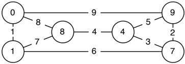
Consider, for example, finding a graceful labelling of a graph. A graceful labelling is a labelling of the vertices of a graph with distinct integers 0 to e such that the e edges (which are labelled with the absolute differences of the labels of the two connected vertices) are also distinct. Graceful labellings have applications in radio astronomy, communication networks, X-ray crystallography, coding theory and elsewhere. Here is the graceful labelling of the graph K 3 × P 2 :

A straight forward model for graceful labelling a graph has variables for the vertex labels, and values which are integers 0 to e . This model has a simple value symmetry as we can map every value i onto e -i . In [16], Puget breaks this value symmetry for K 3 × P 2 with the following ordering constraints:

Note that all the Z j take different values as each integer first occurs in the graph at a different index. Hence, we have a sequence of variables on which there is both an ALLDIFFERENT and precedence constraints.

4 ALLDIFFPREC

Motivated by such examples, we propose the global constraint:

Where E is a set containing pairs of variable indices. This ensures X i = X j for any 1 ≤ i < j ≤ n and X j < X k for any ( j, k ) ∈ E . Without loss of generality, we assume that E does not contain cycles. If it does, the constraint is trivially unsatisfiable. It is not hard to see that decomposition of this global constraint into separate ALLDIFFERENT and binary ordering constraints can hinder propagation.

glyph[negationslash]

Lemma 1 Domain consistency on the constraint ALLDIFFPREC ([ X 1 , . . . , X n ] , E ) is stronger than domain consistency on the decomposition into ALLDIFFERENT ([ X 1 , . . . , X n ]) and the binary ordering constraints, X i < X j for ( i, j ) ∈ E . Bounds consistency on ALLDIFFPREC ([ X 1 , . . . , X n ] , E ) is stronger than bounds consistency on the decomposition, whilst range consistency on ALLDIFFPREC ([ X 1 , . . . , X n ] , E ) is stronger than range consistency on the decomposition.

Proof: Consider ALLDIFFPREC ([ X 1 , X 2 , X 3 ] , { (1 , 3) , (2 , 3) } ) with D ( X 1 ) = D ( X 2 ) = { 1 , 2 , 3 } and D ( X 3 ) = { 2 , 3 , 4 } . Then the decomposition into ALLDIFFERENT ([ X 1 , X 2 , X 3 ]) and the binary ordering constraints, X 1 < X 3 , and X 2 < X 3 is domain consistent. Hence, it is also range and bounds consistent. However, enforcing bounds consistency directly on the global ALLDIFFPREC constraint will prune 2 from the domain of X 3 since this assignment has no bound support. Similarly, enforcing range or domain consistency will prune 2 from the domain of X 3 . ✷

A simple greedy method will find a bound support for the ALLDIFFPREC constraint. This method is an adaptation of the greedy method to build a bound support of the ALLDIFFERENT constraint. For simplicity, we suppose that E contains the transitive closure of the precedence constraints. In fact, this step is not required but makes our argument easier. First, we need to preprocess variables domains so that they respect the precedence constraints X i < X j , ( i, j ) ∈ E : min( X i ) < min( X j ) and max( X i ) < max( X j ) . However, we notice that it is sufficient to enforce a weaker condition on bounds of variables X i and X j such that min( X i ) ≤ min( X j ) and max( X i ) ≤ max( X j ) . If these conditions on variables domains are satisfied then we say that domains are preprocessed . Second, we construct a satisfying assignment as follows. We process all values in the increasing order. When processing a value v , we assign v to the variable with the smallest upper bound, u that has not yet been assigned and that contains v in its domain. Suppose, there exists a set of variables that have the upper bound u , so that X ′ = { X i | D ( X i ) = [ v, u ] } . To construct a solution for ALLDIFFERENT, we would break these ties arbitrarily. In this case, however, we select a variable that is not successor of any variable in the set X ′ . Such a variable always exists, as the transitive closure of the precedence graph does not contain cycles. By the correctness of the original algorithm the resulting assignment is a solution. In addition to satisfying the ALLDIFFERENT constraint, this solution also satisfies the precedence constraints. Indeed, for the constraint X i < X j , the upper bound of D ( X i ) is necessarily smaller than or equal to the upper bound of D ( X j ) . In the case of equality, we tie break in favor of X i . Therefore, a value is assigned to X i before a value gets assigned to X j . Since we process values in increasing order, we obtain X i < X j as required.

Example 1 Consider ALLDIFFPREC ([ X 1 , X 2 , X 3 , X 4 ] , { (1 , 3) , (2 , 3) , (1 , 4) , (2 , 4) } ) with D ( X 1 ) = D ( X 2 ) = { 1 , 2 , 3 , 4 , 5 } , D ( X 3 ) = { 1 , 2 , 3 } and D ( X 4 ) = { 2 , 3 , 4 } . First, we preprocess domains to ensure that min( X i ) ≤ min( X j ) and max( X i ) ≤ max( X j ) , i ∈ { 1 , 2 } , j ∈ { 3 , 4 } . This gives D ( X 1 ) = D ( X 2 ) = D ( X 3 ) = { 1 , 2 , 3 } , D ( X 4 ) = { 2 , 3 , 4 } . As in the greedy algorithm, we consider the first value 1 . This value is contained in domains of variables X 1 , X 2 and X 3 . As max( X 1 ) = max( X 2 ) = max( X 3 ) = 3 , by tie breaking we select variables that are not successors of any other variables among variables { X 1 , X 2 , X 3 } . There are two such variables: X 1 and X 2 . We break this tie arbitrarily and set X 1 to 1. The new domains are D ( X 1 ) = 1 , D ( X 2 ) = D ( X 3 ) = { 2 , 3 } , D ( X 4 ) = { 2 , 3 , 4 } . The next value we consider is 2 . Again, there exist two variables that contain this value, and they have the same upper bounds. By tie-breaking, we select X 2 . Finally, we assign X 3 and X 4 to 3 and 4 respectively.

We can design a filtering algorithm based on this satisfiability test. By successively reducing a variable domain in halves with a binary search we can filter the lower and upper bounds of a variable domain with O ( log d ) tests where d is the cardinality of the domain. Consider, for example, a variable X with the domain D ( X ) = [ l, u ] . We are looking for a support for min( X ) . At the first step we temporally fix the domain of X to the first half so that D ( X ) = [ l, ( u -l ) / 2] and run the bounds disentailment detection algorithm. If this algorithm fails, we halved the search and repeat with the other half. If this algorithm does not fail, we know that there is a value in [ l, ( u -l ) / 2] that has a bounds support. Hence, we continue with the binary search within this half. As each test takes O ( n ) time and there are n variables to prune, the total running time is O ( n 2 log d ) . In the rest of this paper, we improve on this using sophisticated algorithmic ideas.

5 Bounds consistency

We present an algorithm that enforces bounds consistency on the ALLDIFFPREC constraint. First, we consider an assignment X i = v and a partial filtering that this assignment causes. We call this filtering direct pruning caused by the assignment X i = v or, in short, direct pruning of X i = v . Informally, direct pruning works as follows. If X i takes v then the value v becomes unavailable for the other variables due to the ALLDIFFERENT constraint. Hence, we remove v from the domains of variables that have v as their lower bound or upper bound. Due to precedence constraints, we increase the lower bounds of successors of X i to v + 1 and decrease the upper bounds of predecessors of X i to v -1 . Note that direct pruning does not enforce bounds consistency on either ALLDIFFPREC or the single ALLDIFFERENT constraint. However, direct pruning is sufficient to detect bounds inconsistency as we show below.

Let P ( i ) and S ( i ) be the sets of variables that precede and succeed X i , respectively. We denote the domains obtained after direct pruning of X i = v as D dp v ( X 1 ) , . . . , D dp v ( X n ) , so that for all j = 1 , . . . , n :

glyph[negationslash]

These bounds could be pruned further but we will first analyze the properties that this simple filtering offers.

Example 2 Consider ALLDIFFPREC ([ X 1 , X 2 , X 3 ] , { (1 , 2) } ) constraint with D ( X 1 ) = { 1 , 2 } , D ( X 2 ) = { 2 , 3 } , D ( X 3 ) = { 1 , 2 , 3 } . For example, an assignment X 1 = 2 results in the domains: D dp 2 ( X 1 ) = { 2 } , D dp 2 ( X 2 ) = { 3 } and D dp 2 ( X 3 ) = { 1 , 2 , 3 } . We point out again that we can continue pruning as values 2 and 3 have to be removed from D dp 2 ( X 3 ) . However, direct pruning of X 1 = 2 is sufficient for our purpose. Consider another example. An assignment X 3 = 1 results in the domains: D dp 3 ( X 1 ) = { 2 } , D dp 3 ( X 2 ) = { 2 , 3 } and D dp 3 ( X 3 ) = { 1 } .

Our algorithm is based on the following lemma.

Lemma 2 Let ALLDIFFERENT and precedence constraints be bounds consistent over variables X , X i = v , v ∈ { min( X i ) , max( X i ) } be an assignment of a variable X i to its bound and D dp v ( X 1 ) , . . . , D dp v ( X n ) be the domains after direct pruning of X i = v . Then, X i = v is bounds consistent iff ALLDIFFERENT ([ X 1 , . . . , X n ]) , where domains of variables X are D dp v ( X 1 ) , . . . , D dp v ( X n ) , has a solution.

Proof: Suppose ALLDIFFERENT and the precedence constraints are bounds consistent. As precedence constraints are bounds consistent, we know that for all ( i, j ) ∈ E , X i < X j , min( X i ) < min( X j ) and max( X i ) < max( X j ) . Consider direct pruning of X i = v . Note, direct pruning of X i = v preserves the property of domains being preprocessed. The pruning can only create equality of lower bounds or upper bounds for some precedence constraints. The assignment X 3 = 1 demonstrates this situation in Example 2. Direct pruning of X 3 = 1 forces lower bounds of X 1 and X 2 , that are in the precedence relation, to be equal.

As domains D dp v ( X 1 ) , . . . , D dp v ( X n ) are preprocessed, we know that the greedy algorithm (Section 4) will find a solution of ALLDIFFERENT on the domains D dp v ( X 1 ) , . . . , D dp v ( X n ) that also satisfies the precedence constraints if a solution exists. This solution is a support for X i = v . glyph[intersectionsq] glyph[unionsq]

Based on Lemma 2 we prove that we can enforce bounds consistency on the ALLDIFFPREC constraint in O ( n 2 ) . However, we start with a simpler and less efficient algorithm to explain the idea . We show how to improve this algorithm in the next section. Given Lemma 2, the most straightforward algorithm to enforce bounds consistency for X i = v is to assign X i to v , perform the direct pruning, run the greedy algorithm and, if it fails, prune v . Interestingly enough, to detect bounds disentailment we do not have to run a greedy algorithm for each pair X i = v . If the ALLDIFFERENT constraint and the precedence constraints are bounds consistent, we show that it is sufficient to check that a set of conditions (5)-(10) holds for each interval of values. If these conditions are satisfied then the pair X i = v is bounds consistent. Hence, for each pair X i = v , 1 ≤ i ≤ n , v ∈ D ( X i ) , and for each interval we enforce the following conditions. We assume that ∪ n i =1 D ( X i ) = [1 , d ] . For X i , 1 ≤ i ≤ n , v ∈ D ( X i ) and for all intervals [ v, v + k ] and [ v -p, v ] , k ∈ [max( X i ) -v + 1 , d -v ] and p ∈ [ v -min( X i ) + 1 , v -1] , the following conditions have to be satisfied:

Note that we actually do not have to consider all possible intervals. For every variable-value pair X i = v we consider all intervals [ v, u ] , u ∈ [max( X i ) + 1 , d ] and all intervals [ l, v ] , l ∈ [1 , min( X i ) -1] . The parameter k ( p ) is used to slide between intervals [ v, u ] , u ∈ [max( X i ) + 1 , d ] ([ l, v ] , l ∈ [1 , min( X i ) -1]) . Equations (5)-(7) make sure that the number of variables that fall into an interval [ v, u ] , after the assignment X i to v , is less than or equal to the length of the interval minus 1. Symmetrically, Equations (8)-(10) ensure that the same condition is satisfied for all intervals [ l, v ] . If there exists an interval [ v, u ] ( [ l, v ] ) that violates the condition for a pair X i = v then this interval is removed from D ( X i ) .

Example 3 Consider ALLDIFFPREC ([ X 1 , X 2 , X 3 , X 4 , X 5 ] , { (1 , 2) , (1 , 3) } ) . Domains of the variables are D ( X 1 ) = [1 , 5] , D ( X 2 ) = D ( X 3 ) = [2 , 6] and D ( X 4 ) = D ( X 5 ) = [3 , 6] . Consider a variable-value pair X 1 = 3 . By the direct pruning we get the following domains: D dp 3 ( X 1 ) = 3 , D dp 3 ( X 2 ) = [4 , 6] , D dp 3 ( X 3 ) = [4 , 6] ,

D dp 3 ( X 4 ) = [4 , 6] and D dp 3 ( X 5 ) = [4 , 6] . The interval [4 , 6] is a violated Hall interval as it contains four variables. We show that Equations (5) -(6) detect that the interval [3 , 6] has to be pruned from D ( X 1 ) .

Consider the pair X 1 = 3 and the interval [ v, v + k ] , where v = 3 , k = 3 . We get that B 1 1 , 6 = |{ j ∈ { 2 , 3 }|D ( X j ) ⊆ [1 , 6] }| = 2 D 1 3 , 6 = |{ j ∈ { 4 , 5 } ) |D ( X j ) ⊆ [3 , 6] }| = 2 and B 1 1 , 6 + D 1 3 , 6 = 4 which is greater than k = 3 . Hence, the interval [3 , 6] has to be removed from D ( X 1 ) .

Theorem 1. Consider the ALLDIFFERENT [ X 1 , . . . , X n ] constraint and a set of precedence constraints X i < X j . Enforcing conditions (5) -(10) together with bounds consistency on the ALLDIFFERENT constraint and the precedence constraints is equivalent to enforcing bounds consistency on the ALLDIFFPREC constraint.

Proof: Suppose conditions (5)-(10) are fulfilled, ALLDIFFERENT and precedence constraints are bounds consistent and the ALLDIFFPREC constraint is not bounds consistent. Let an assignment of a variable X i to its bound max( X i ) be an unsupported bound. We denote max( X i ) v to simplify notations. We recall that we denoted the domains after direct pruning of X i = v D dp v ( X 1 ) , . . . , D dp v ( X n ) . By Lemma 2 the ALLDIFFERENT ([ X 1 , . . . , X n ]) constraint where domains of variables X are D dp v ( X 1 ) , . . . , D dp v ( X n ) fails. Hence, there exists a violated Hall interval [ l, u ] such that |D dp v ( X i ) ⊆ [ l, u ] }| > u -l +1 .

Note that direct pruning of X i = v does not cause the pruning of variables in P ( i ) , as all precedence constraints are bounds consistent on the original domains. Next we consider several cases depending on the relative position of the value v and the violated Hall interval on the line. Note that the interval [ l, u ] was not a violated Hall interval before the assignment X i = v . However, due to direct pruning of X i = v a number of additional variables domains can be forced to be inside [ l, u ] . Hence, we analyze these additional variables and show that conditions (5)-(10) prevent the creation of a violated Hall interval.

Case 1. Suppose v ∈ [ l, u ] . As [ l, u ] is a violated Hall interval, we have that

Note that the number of additional variables that fall into the interval [ l, u ] after setting X i to v consists only of variables that succeed X i , such that D ( X j ) ⊆ [1 , u ] . Hence, |{ j / ∈ S ( i ) |D dp v ( X j ) ⊆ [ l, u ] }| = |{ j / ∈ S ( i ) |D ( X j ) ⊆ [ l, u ] }| , |{ j / ∈ S ( i ) |D dp v ( X j ) ⊆ [ l, u ] }| = |{ j ∈ S ( i ) |D ( X j ) ⊆ [1 , u ] }| and

which violate conditions (5)-(7) for v = l and k = u -l .

Case 2. Suppose v / ∈ [ l, u ] . If v > u + 1 or v < l -1 , the assignment X i = v does not force any extra variables to fall into the interval [ l, u ] . Hence, the interval [ l, u ] is a violated Hall interval before the assignment. This contradicts that ALLDIFFERENT is bounds consistent.

Case 3. Suppose v = u + 1 . In this case the assignment X i = v does not force any additional variables among successors to fall into [ l, u ] , as D dp v ( X j ) ⊆ [ u +2 , d ] . Note that there are no successors that are contained in the interval [1 , v ] , because precedence constraints are bounds consistent. Therefore, |{ j ∈ S ( i ) |D ( X j ) ⊆ [ l, v ] }| = 0 . Hence, the only additional variables that fall into [ l, u ] are variables that do not have a precedence relation with X i and v = max( X j ) = u + 1 , so |{ j | j / ∈ S ( i ) , D dp v ( X j ) ⊆ [ l, u ] }| = |{ j | j / ∈ S ( i ) , D ( X j ) ⊆ [ l, u +1] }| . As [ l, u ] is a violated Hall interval, we have

This contradicts Equation (10) |{ j ∈ S ( i ) |D ( X j ) ⊆ [ l, u + 1] }| + |{ j | j / ∈ S ( i ) , D ( X j ) ⊆ [ l, u + 1] }| ≤ ( u + 1) -l as the first term equals 0 in the equation by the argument above.

Case 4. Suppose v = l -1 . In this case the set of additional variables that fall into the interval [ l, u ] consists of two subsets of variables. The first set contains variables that succeed X i , such that D ( X j ) ⊆ [ l ′ , u ] , l ′ < v and D dp v ( X j ) ⊆ [ l, u ] . The second set contains the variables that do not have precedence relation with X i and v = max ( X j ) = l -1 . Consider the interval [ l -1 , u ] . As conditions (5)-(7) are satisfied for the interval [ l -1 , u ] , we get that

On the other hand, as the [ l, u ] is violated we have

We know that |{ j / ∈ S ( i ) |D ( X j ) ⊆ [ l -1 , u ] }| = |{ j | j / ∈ S ( i ) , D dp v ( X j ) ⊆ [ l, u ] }| and |{ j ∈ S ( i ) |D ( X j ) ⊆ [1 , u ] }| = |{ j ∈ S ( i ) |D dp v ( X j ) ⊆ [ l, u ] }| by the construction of the direct pruning. This leads to a contradiction between the last two inequalities.

Therefore, the interval [ l, u ] cannot be a violated Hall interval. Similarly, we can prove the same result for the minimum value of X j .

The reverse direction is trivial.

glyph[intersectionsq]

glyph[unionsq]

Theorem 1 proves that conditions (5)-(10) together with bounds consistency on the ALLDIFFERENT constraint and the precedence constraints are necessary and sufficient conditions to enforce bounds consistency on the ALLDIFFPREC constraint. The time complexity of enforcing these conditions in O ( nd 2 ) , as for each variable we check O ( d 2 ) intervals. This time complexity can be reduced by making an observation, that we do not need to check intervals of length greater than n as conditions are trivially satisfied for such intervals. This reduces the complexity to O ( n 2 d ) .

We make an observation that helps to further reduce the time complexity of enforcing these conditions. We denote L the set of all minimum values in variables domains L = ∪ n i =1 { min( D ( X i )) } and U the set of all maximum values in variables domains U = ∪ n i =1 { max( D ( X i )) } . Let [ l, u ] be an interval that violates the conditions. We denote c l,u the amount of violation in this interval: c l,u = B i 1 ,u + D i l,u -( u -l ) .

Observation 1 Let X i be a variable and [ v, v + k ] , v ∈ D ( X i ) be an interval that violates conditions (5) -(7) . Then there exists a violated interval [ l, u ] such that [ l, u ] ⊆ [ v, v + k ] , l, u ∈ L ∪ U and c l,u > l -v .

Proof: Consider a violated interval [ v, v + k ] . In this case B i 1 ,v + k + D i v,v + k > k . There exists an interval [ l, u ] ⊆ [ v, v + k ] such that l, u ∈ L ∪ U . We take the largest interval [ l, u ] . Note that such an interval always exists as the interval [max( X i ) , max( X i )] is contained inside the interval [ v, v + k ] . The interval [ l, u ] also violates the conditions, because it contains the same variables. So, we have B i 1 ,u + D i l,u > u -l . We note that D i l,u = D i v,v + k as there are no lower bounds in the interval [ v, l ) . Similarly, there are no upper bounds in the interval ( u, v + k ] . Hence, B i 1 ,u = B i 1 ,v + k . Therefore, B i 1 ,u + D i l,u > k . The value c l,u is greater than k -u + l ≥ v + k -v -u + l ≥ v + k -u + l -v ≥ l -v as u ≤ v + k .

glyph[intersectionsq]

glyph[unionsq]

Observation 1 shows that it is sufficient to check intervals [ v, v + k ] , { v, v + k } ∈ L ∪ U . We can infer all pruning from these intervals. Let [ l, u ] , l, u ∈ L ∪ U be an interval that violates conditions (5)-(7) for a variable X i and c l,u be the violation cost. Then we remove the interval [ l -( c l,u -1) , u ] from D ( X i ) , as any interval between [ l -( c l,u -1) , u ] and [ l, u ] is a violated interval. A dual observation holds for conditions (8)-(10). This reduces the time complexity of checking (5)-(10) to O ( n 3 ) .

6 Faster bounds consistency algorithm

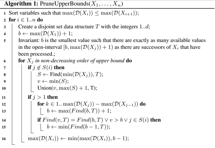
Observation 1 allows us to construct a faster algorithm to enforce conditions (5)-(10). First, we observe that the conditions can be checked for each variable independently. Consider a variable X i . We sort all variables X j , j = 1 , . . . , n in a non-decreasing order of their upper bounds. When processing a variable X j , j / ∈ S ( i ) , we assign X j to the smallest value that has not been taken. When processing a variable X j , j ∈ S ( i ) , we store information about the number of successors that we have seen so far. We perform pruning if we find an interval [ l, u ] such that the number of available values in this interval equals the number of successors in the interval [1 , u ] . We use a disjoint set data structure to perform counting operations in O ( d ) time.

Algorithm 1 shows a pseudocode of our algorithm. We denote T a disjoint set data structure. The function Find ( v 1 , T ) returns the set that contains the value v 1 . The function Union ( v 1 , v 2 , T ) joins the values v 1 and v 2 into a single set. We use a disjoint set union data structure [22] that allows to perform Find and Union in O (1) time.

Theorem 1 Algorithm 1 enforces conditions (5) -(7) in O ( nd ) time.

Proof: Enforcing conditions (5)-(7) on the i th variable corresponds to the i th loop (line 2). Hence, we can consider each run independently.

Wedenote I j a set of values that are taken by non-successors of X i after the variable X j is processed. The algorithm maintains a pointer b that stores the minimum value such that the number of available values in the interval [ b, max( X j ) + 1) is equal to B i 1 ,max ( X j ) after the variable X j is processed.

Invariant . We prove the invariant for the pointer b by induction. The invariant holds at step j = 0 . Note that the first variable can not be a successor of X i . Indeed, b = max ( X 1 ) + 1 and the interval [max( X 1 ) + 1 , max( X 1 ) + 1) is empty. Let us assume that the invariant holds after processing the variable X j -1 .

Suppose the next variable to process is X j . After we assigned X j to a value, we move b forward to capture a possible increase of the upper bound from max( X j -1 ) to max( X j ) (line 13) and, then, backward if either X j is a successor of X i or X j is a non-successor and X j takes a value v such that b ≤ v (line 15). Note, that when we move b , we ignore values in I j . To point this out we call steps of b available-value-steps. Thanks to a disjoint set union data structure we can jump over values in I j in O (1) per step [22].

Moving forward . We move the pointer b on max( X j ) -max( X j -1 ) availablevalue-steps forward. We denote b ′ a new value of b . The line 13 ensures that the number of available values in the interval [ b ′ , max( X j ) + 1) equals to the number of available values in the interval [ b, max( X j -1 ) + 1) . This operation preserves the invariant by the induction hypothesis.

Moving backward . We consider two cases.

Case 1. X j is a successor of X i . In this case, we move b ′ one available-value-step backward to capture that X j is a successor (line 15). This preserves the invariant.

Case 2. X j is not a successor of X i . Suppose v and b ′ are in the same set, so that Find ( v, T ) = Find ( b, T ) . Then we move b ′ to the minimum element in this set. This step does not change the number of available values between the pointer b ′ and max( X j ) . However, it makes sure that b ′ stores the minimum possible value. This preserves the invariant.

Suppose v and b ′ are in different sets. If v > b ′ then we move b ′ one availablevalue-step backward, as v took one of the available values in [ b ′ , max( X j ) + 1) . This preserves the invariant. If v < b ′ then the invariant holds by the induction hypothesis. Hence, the new value of b preserves the invariant.

Note that the length of the interval [ b, max( X j ) + 1) equals the sum of B i 1 , max( X j ) and D b, max( X j ) due to the invariant. This means that the interval [ b, max( X j ) + 1) violates conditions (5)-(7), as the sum B i 1 , max( X j ) + D b, max( X j ) has to be less than or equal to the length of the interval [ b, max( X j ) + 1) minus 1.

Soundness . Suppose we pruned an interval [ b -1 , max( X j )] from D ( X i ) after the processing of the variable X j . This pruning is sound because the interval [ b, max( X j )+ 1) violates conditions (5)-(7).

Completeness . Suppose there exists an interval [ l, u ] that violates conditions (5)(7), so that B i 1 ,u + D i l,u > u -l . However, the algorithm does not prune the upper bound of X i to l -1 . Suppose that l ∈ L , u ∈ U . As the pointer b preserves the invariant, there are exactly B i 1 ,u available values between [ l, u +1) . Hence b points to l and max( X i ) ≤ l -1 .

Suppose that l / ∈ L , u ∈ U . We consider the step when the last pruning of the variable X i occurs. Suppose we processed the variable X j at this step. The pointer b stores max( X i ) + 1 . As b does not move backward in the following steps, we conclude that neither successors nor non-successors with domains that are contained inside the interval [ b, d ] occur. Hence, B i 1 ,u + D i l,u = B i 1 ,u + D i max( X i )+1 ,u , max( X j ) ≤ u , u ∈ U , l < max( X i ) . Hence [ l, u ] is not a violated interval.

Complexity . At each iteration of the loop (line 2) the pointer b moves O ( d ) times forward and O ( n ) times backward. Due to a disjoint set data structure the total cost of the operations is O ( d ) , the functions Union ( v 1 , v 2 , T ) and Find ( v 1 , T ) take O (1) [22]. The total time complexity is O ( nd ) . glyph[intersectionsq] glyph[unionsq]

We can construct a similar algorithm to Algorithm 1 to enforce conditions (8)-(10) and prune lower bounds.

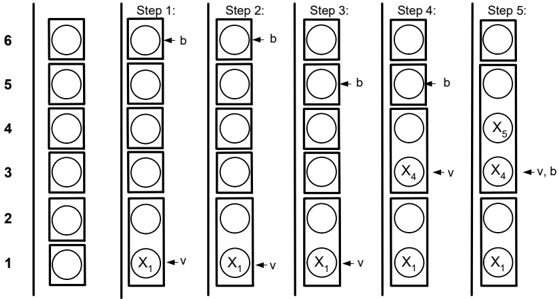
Example 4 Consider ALLDIFFPREC ([ X 1 , X 2 , X 3 , X 4 , X 5 ] , { (1 , 2) , (1 , 3) } ) for Example 3. We show how our algorithm works on this example.

We represent values in the disjoint set data structure T with circles. We use rectangles to denote sets of joint values. Initially, all values are in disjoint sets. If a variable

X i takes a value v we put the label X i in the v th circle. Figure 6 shows five steps of the algorithm when processing the variable X 1 (line 2, i = 1 ).

Consider the first step. We set v = 1 as min( X 1 ) is 1. We join the values 1 and 2 into a single set (line 10). The pointer b is set to max( X 1 )+1 = 6 . Consider the second step. We process the variable X 2 which is a successor of X 1 . As max( X 2 ) -max( X 1 ) = 1 we move b one available-value-step forward, b = 7 . However, as X 2 is a successor, we move b available-value-step backward. Hence, b = 6 . Consider the third step. We process X 3 which is a successor of X 1 . As max( X 3 ) -max( X 2 ) = 0 we do not move b forward. However, as X 3 is a successor, we move b available-value-step backward, b is set to 5. Consider the fourth step. We process X 4 which is a non-successor of X 1 . The value min( X 4 ) is 3. Hence, v = 3 and join 3 and 4 into a single set. Consider the fifth step. We process the variable X 5 which is a non-successor of X 1 . The value min( X 5 ) is 4, as the value 3 is taken by X 4 . As values 3 and 4 are in the same set, we do not move v and join { 3 , 4 } and 5 into a set. Note that v and b are in the same set and we move b to the minimum element in this set. Hence, b = 3 and we prune [3 , 5] from X 1 .

The complexity of the algorithm can be reduced to O ( n 2 ) . Let L be the set of domain lower bounds sorted in increasing order and let l i -1 and l i be two consecutive values in that ordering. Following [6], we initialize the disjoint set data structures with only the elements in L . We assign a counter c i to each element l i initialized to the value l i -l i -1 . Line 10 of the algorithm can be modified to decrement the counter of max( S ) . The algorithm calls the function Union only if the counter of max( S ) is decremented to zero. The algorithm preserves its correctness and since there are at most n elements in L , the factor d in the complexity of the algorithm is replaced by n resulting in a running time complexity of O ( n 2 ) .

7 Bounds consistency decomposition

We present a decomposition of the ALLDIFFPREC constraint. For 1 ≤ i ≤ n , 1 ≤ l ≤ u ≤ d and u -l < n , we introduce Boolean variables B il and A ilu and post the following constraints:

Theorem 2. Enforcing bounds consistency on constraints (11) and (17) enforces bounds consistency on the corresponding ALLDIFFPREC constraint in O ( n 2 d 2 ) down a branch of the search tree.

Proof: Constraints (11)-(13) enforce bounds consistency on the ALLDIFFERENT constraint. Constraints (16)-(17) enforce bounds consistency on the precedence constraints. Finally, conditions (8)-(10) are captured by constraints (14) and (15). By Theorem 1, enforcing BC on ALLDIFFERENT, precedence constraints and enforcing conditions (8)-(10) is sufficient to enforce bounds consistency on the ALLDIFFPREC constraint. The time complexity is dominated by O ( nd 2 ) linear inequality constraints (14)(15). It takes O ( n ) time to propagate a linear inequality constraint over O ( n ) Boolean variables down a branch of the search tree. Hence, the total complexity is O ( n 2 d 2 ) . ✷

Note that the time complexity of decomposition contains a factor d that we cannot reduce as in the case of the conditions (5)-(10). As we compute the time complexity down a branch of a search tree we have to consider all possible O ( d 2 ) tight intervals that might emerge during the search.

8 Domain consistency

glyph[negationslash]

Whilst enforcing bounds consistency on the ALLDIFFPREC constraint takes just low order polynomial time, enforcing domain consistency is intractable in general (assuming P = NP ).

Theorem 2 Enforcing domain consistency on ALLDIFFPREC ([ X 1 , . . . , X n ] , E ) is NP-hard.

Proof: We give a reduction from 3-SAT. Suppose we have a 3-SAT problem in N variables and M clauses. We consider an ALLDIFFPREC constraint on 2 N +3 M variables. The first 2 N variables represent a truth assignment. The next 3 M variables represent the literals which satisfy each of the clauses. For 1 ≤ i ≤ N , the variables X 2 i -1 and X 2 i have domains { i, N + M + i } . X 2 i -1 = i corresponds to the case in which we have a truth assignment that assigns x i to false whilst X 2 i = i corresponds to the case in which we have a truth assignment that assigns x i to true. The all different constraint ensures that only one of X 2 i -1 and X 2 i can be assigned to i . Hence one of these two cases must hold. For 1 ≤ i ≤ M , the variables X N +3 i -2 , X N +3 i -1 and X N +3 i represent the three literals in each clause. The values assigned to these variables will ensure that the truth assignment satisfies at least one literal in each clause. The domains of X N +3 i -2 , X N +3 i -1 and X N +3 i are { N + i, 2 N + M +2 i, 2 N + M +2 i -1 , } . N + i will be the value used to indicate that the corresponding literal satisfies the clause. For each literal in a clause, we add an edge to E to ensure that there is an ordering constraint between one of the first 2 N variables in the truth assignment section and the corresponding variable in the clause section. For example, suppose the i th clause is x j ∨¬ x k ∨ x l then we add 3 edges to E to ensure: X 2 j < X N +3 i -2 , X 2 k -1 < X N +3 i -1 , and X 2 l < X N +3 i . The all different constraint ensures one of X N +3 i -2 , X N +3 i -1 and X N +3 i takes the smallest value N + i , and the ordering constraint then checks that the corresponding literal is set to true. By construction, the ALLDIFFPREC constraint has support iff there is a satisfying assignment to the original 3-SAT problem. ✷

Note that the proof uses a DAG defined by E that is flat, and does not contain any chains. Hence, enforcing domain consistency on ALLDIFFPREC remains NP-hard without chains of precedences. Note also that SAT remains NP-hard even if each clause has at most 3 literals, and each literal or negated literal occurs at most three times. Hence, a similar reduction shows that enforcing domain consistency on ALLDIFFPREC remains NP-hard even if the degree of nodes in E is at most 3 (that is, we have at most 3 precedence constraints on any variable).

9 Other related work

There have been many studies on propagation algorithms for a single ALLDIFFERENT constraint. A domain consistency algorithm that runs in O ( n 2 . 5 ) was introduced in [2]. A range consistency algorithm was then proposed in [3] that runs in time O ( n 2 ) . The focus was moved from range consistency to bound consistency with [4], who proposed a bounds consistency algorithm that runs in O ( n log n ) . This was later improved further in [17] and then in [6].

Decompositions that achieve bounds consistency have been given for a number of global constraints. Relevant to this work, similar decompositions have been given for a single ALLDIFFERENT constraint [18], as well as for overlapping ALLDIFFERENT constraints [19]. These decompositions have the property that enforcing bound consistency on the decomposition achieves bounds consistency on the original global constraint.

Anumber of global constraints have been combined together and specialized propagators developed to deal with these conjunctions. For example, a global lexicographical ordering and sum constraint have been combined together [20]. As a second example, a generic method has been proposed for propagating combinations of the global lexicographical ordering and a family of globals including the REGULAR and SEQUENCE constraints [21].

10 Conclusions

We have proposed a new global constraint that combines together an ALLDIFFERENT constraint with precedence constraints that strictly order given pairs of variables. We gave an efficient propagation algorithm that enforces bounds consistency on this global constraint in O ( n 2 ) time, and showed how this propagator can be simulated with a simple decomposition extends the bounds consistency enforcing decomposition proposed for the ALLDIFFERENT constraint. Finally, we proved that enforcing domain consistency on this global constraint is NP-hard in general. There are many interesting future directions. We could, for example, study the convex hull of the ALLDIFFPREC constraint. Other interesting future work includes studying the combination of precedence constraints with generalizations of the ALLDIFFERENT constraint including the global cardinality constraint and the inter-distance constraint.

References

1. Lauriere, J.L.: ALICE: a language and a program for stating and solving combinatorial problems. artificial intelligence. Artificial Intelligence 10 (1978) 29-127
2. R´ egin, J.C.: A filtering algorithm for constraints of difference in CSPs. In: Proceedings of the 12th National Conference on AI, Association for Advancement of Artificial Intelligence (1994) 362-367
3. Leconte, M.: A bounds-based reduction scheme for constraints of difference. In: Proceedings of Second International Workshop on Constraint-based Reasoning (Constraint-96). (1996)
4. Puget, J.: A fast algorithm for the bound consistency of alldiff constraints. In: 15th National Conference on Artificial Intelligence, Association for Advancement of Artificial Intelligence (1998) 359-366
5. Mehlhorn, K., Thiel, S.: Faster algorithms for bound-consistency of the sortedness and the alldifferent constraint. Sixth International Conference on Principles and Practice of Constraint Programming (2000)
6. Lopez-Ortiz, A., Quimper, C., Tromp, J., van Beek, P.: A fast and simple algorithm for bounds consistency of the alldifferent constraint. In: Proceedings of the 18th International Conference on AI, International Joint Conference on Artificial Intelligence (2003)
7. Stergiou, K., Walsh, T.: The difference all-difference makes. In: Proceedings of 16th IJCAI, International Joint Conference on Artificial Intelligence (1999)
8. Milano, M., Ottosson, G., Refalo, P., Thorsteinsson, E.: The role of integer programming techniques in constraint programming's global constraints. INFORMS Journal on Computing 14 (2002) 387-402
9. Williams, H., Yan, H.: Representations of the all different predicate of constraint satisfaction in integer programming. INFORMS Journal on Computing 13 (2001) 96-103
10. Walsh, T.: Constraint patterns. In Rossi, F., ed.: 9th International Conference on Principles and Practices of Constraint Programming (CP-2003), Springer (2003)
11. Beldiceanu, N., Bourreau, E., David Rivreau Helmut Simonis Solving Resource-constrained Project Scheduling Problems with CHIP. 5th International Workshop on Project Management and Scheduling (PMS'96), Poznan. (1996) 35-38.
12. Simonis, H.: Building Industrial Applications with Constraint Programming. Constraints in Computational Logics: Theory and Applications, International Summer School, CCL'99, Springer (2001)
13. Debruyne, R., Bessi` ere, C.: Some practicable filtering techniques for the constraint satisfaction problem. In: Proceedings of the 15th IJCAI, International Joint Conference on Artificial Intelligence (1997) 412-417
14. Garey, M., Johnson, D., Simons, B., Tarjan, R.: Scheduling unit-time tasks with arbitrary release times and deadlines. SIAM J. Comput. 10 (1981) 256-269
15. Puget, J.F.: Breaking all value symmetries in surjection problems. In van Beek, P., ed.: Proceedings of 11th International Conference on Principles and Practice of Constraint Programming (CP2005), Springer (2005)
16. Puget, J.F.: Symmetry in injective problems. Constraint Programming Letters 3 (2007) 1-20
17. Mehlhorn, K., Thiel, S.: Faster algorithms for bound-consistency of the sortedness and the alldifferent constraint. In: CP '02: Proceedings of the 6th International Conference on Principles and Practice of Constraint Programming, Springer-Verlag (2000) 306-319
18. Bessiere, C., Katsirelos, G., Narodytska, N., Quimper, C.G., Walsh, T.: Decompositions of all different, global cardinality and related constraints. In: Proceedings of 21st IJCAI, International Joint Conference on Artificial Intelligence (2009) 419-424
19. Bessiere, C., Katsirelos, G., Narodytska, N., Quimper, C.G., Walsh, T.: Propagating conjunctions of alldifferent constraints. In Fox, M., Poole, D., eds.: Proc. of the Twenty-Fourth AAAI Conference on Artificial Intelligence (AAAI 2010), AAAI Press (2010)
20. Hnich, B., Kiziltan, Z., Walsh, T.: Combining symmetry breaking with other constraints: lexicographic ordering with sums. In: Proceedings of the 8th International Symposium on the Artificial Intelligence and Mathematics. (2004)
21. Katsirelos, G., Narodytska, N., Walsh, T.: Combining symmetry breaking and global constraints. In Oddi, A., Fages, F., Rossi, F., eds.: Recent Advances in Constraints, 13th Annual ERCIM International Workshop on Constraint Solving and Constraint Logic Programming (CSCLP 2008). Volume 5655 of Lecture Notes in Computer Science., Springer (2009) 84-98
22. Gabow, H. and Tarjan, R.: A linear-time algorithm for a special case of disjoint set union. Proceedings of the fifteenth annual ACM symposium on Theory of computing (STOC '83)., ACM(1983) 246-251