The Complexity of Planning Problems With Simple Causal Graphs

Omer Gim´ enez

Dept. de Llenguatges i Sistemes Inform` atics Universitat Polit` ecnica de Catalunya Jordi Girona, 1-3 08034 Barcelona, Spain

Anders Jonsson

Dept. of Information and Communication Technologies Passeig de Circumval · laci´ o, 8 08003 Barcelona, Spain

Abstract

We present three new complexity results for classes of planning problems with simple causal graphs. First, we describe a polynomial-time algorithm that uses macros to generate plans for the class 3S of planning problems with binary state variables and acyclic causal graphs. This implies that plan generation may be tractable even when a planning problem has an exponentially long minimal solution. We also prove that the problem of plan existence for planning problems with multi-valued variables and chain causal graphs is NP-hard. Finally, we show that plan existence for planning problems with binary state variables and polytree causal graphs is NP-complete.

1. Introduction

Planning is an area of research in artificial intelligence that aims to achieve autonomous control of complex systems. Formally, the planning problem is to obtain a sequence of transformations for moving a system from an initial state to a goal state, given a description of possible transformations. Planning algorithms have been successfully used in a variety of applications, including robotics, process planning, information gathering, autonomous agents and spacecraft mission control. Research in planning has seen significant progress during the last ten years, in part due to the establishment of the International Planning Competition.

An important aspect of research in planning is to classify the complexity of solving planning problems. Being able to classify a planning problem according to complexity makes it possible to select the right tool for solving it. Researchers usually distinguish between two problems: plan generation, the problem of generating a sequence of transformations for achieving the goal, and plan existence, the problem of determining whether such a sequence exists. If the original STRIPS formalism is used, plan existence is undecidable in the first-order case (Chapman, 1987) and PSPACE-complete in the propositional case (Bylander, 1994). Using PDDL, the representation language used at the International Planning Competition, plan existence is EXPSPACE-complete (Erol, Nau, & Subrahmanian, 1995). However, planning problems usually exhibit structure that makes them much

[email protected]

[email protected]

easier to solve. Helmert (2003) showed that many of the benchmark problems used at the International Planning Competition are in fact in P or NP.

A common type of structure that researchers have used to characterize planning problems is the so called causal graph (Knoblock, 1994). The causal graph of a planning problem is a graph that captures the degree of independence among the state variables of the problem, and is easily constructed given a description of the problem transformations. The independence between state variables can be exploited to devise algorithms for efficiently solving the planning problem. The causal graph has been used as a tool for describing tractable subclasses of planning problems (Brafman & Domshlak, 2003; Jonsson & B¨ ackstr¨ om, 1998; Williams & Nayak, 1997), for decomposing planning problems into smaller problems (Brafman & Domshlak, 2006; Jonsson, 2007; Knoblock, 1994), and as the basis for domain-independent heuristics that guide the search for a valid plan (Helmert, 2006).

In the present work we explore the computational complexity of solving planning problems with simple causal graphs. We present new results for three classes of planning problems studied in the literature: the class 3S (Jonsson & B¨ ackstr¨ om, 1998), the class C n (Domshlak & Dinitz, 2001), and the class of planning problems with polytree causal graphs (Brafman & Domshlak, 2003). In brief, we show that plan generation for instances of the first class can be solved in polynomial time using macros, but that plan existence is not solvable in polynomial time for the remaining two classes, unless P = NP. This work first appeared in a conference paper (Gim´ enez & Jonsson, 2007); the current paper provides more detail and additional insights as well as new sections on plan length and CP-nets.

A planning problem belongs to the class 3S if its causal graph is acyclic and all state variables are either static , symmetrically reversible or splitting (see Section 3 for a precise definition of these terms). The class 3S was introduced and studied by Jonsson and B¨ ackstr¨ om (1998) as an example of a class for which plan existence is easy (there exists a polynomial-time algorithm that determines whether or not a particular planning problem of that class is solvable) but plan generation is hard (there exists no polynomial-time algorithm that generates a valid plan for every planning problem of the class). More precisely, Jonsson and B¨ ackstr¨ om showed that there are planning problems of the class 3S for which every valid plan is exponentially long. This clearly prevents the existence of an efficient plan generation algorithm.

Our first contribution is to show that plan generation for 3S is in fact easy if we are allowed to express a valid plan using macros . A macro is simply a sequence of operators and other macros. We present a polynomial-time algorithm that produces valid plans of this form for planning problems of the class 3S . Namely, our algorithm outputs in polynomial time a system of macros that, when executed, produce the actual valid plan for the planning problem instance. The algorithm is sound and complete, that is, it generates a valid plan if and only if one exists. We contrast our algorithm to the incremental algorithm proposed by Jonsson and B¨ ackstr¨ om (1998), which is polynomial in the size of the output.

We also investigate the complexity of the class C n of planning problems with multivalued state variables and chain causal graphs. In other words, the causal graph is just a directed path. Domshlak and Dinitz (2001) showed that there are solvable instances of this class that require exponentially long plans. However, as it is the case with the class 3S , there could exist an efficient procedure for generating valid plans for C n instances using

macros or some other novel idea. We show that plan existence in C n is NP-hard, hence ruling out that such an efficient procedure exists, unless P = NP.

We also prove that plan existence for planning problems whose causal graph is a polytree (i.e., the underlying undirected graph is acyclic) is NP-complete, even if we restrict to problems with binary variables. This result closes the complexity gap that appears in Brafman and Domshlak (2003) regarding planning problems with binary variables. The authors show that plan existence is NP-complete for planning problems with singly connected causal graphs, and that plan generation is polynomial for planning problems with polytree causal graphs of bounded indegree. We use the same reduction to prove that a similar problem on polytree CP-nets (Boutilier, Brafman, Domshlak, Hoos, & Poole, 2004) is NP-complete.

1.1 Related Work

Several researchers have used the causal graph to devise algorithms for solving planning problems or to study the complexity of planning problems. Knoblock (1994) used the causal graph to decompose a planning problem into a hierarchy of increasingly abstract problems. Under certain conditions, solving the hierarchy of abstract problems is easier than solving the original problem. Williams and Nayak (1997) introduced several restrictions on planning problems to ensure tractability, one of which is that the causal graph should be acyclic. Jonsson and B¨ ackstr¨ om (1998) defined the class 3S of planning problems, which also requires the causal graphs to be acyclic, and showed that plan existence is polynomial for this class.

Domshlak and Dinitz (2001) analyzed the complexity of several classes of planning problems with acyclic causal graphs. Brafman and Domshlak (2003) designed a polynomialtime algorithm for solving planning problems with binary state variables and acyclic causal graph of bounded indegree. Brafman and Domshlak (2006) identified conditions under which it is possible to factorize a planning problem into several subproblems and solve the subproblems independently. They claimed that a planning problem is suitable for factorization if its causal graph has bounded tree-width.

The idea of using macros in planning is almost as old as planning itself (Fikes & Nilsson, 1971). Minton (1985) developed an algorithm that measures the utility of plan fragments and stores them as macros if they are deemed useful. Korf (1987) showed that macros can exponentially reduce the search space size of a planning problem if chosen carefully. Vidal (2004) used relaxed plans generated while computing heuristics to produce macros that contribute to the solution of planning problems. Macro-FF (Botea, Enzenberger, M¨ uller, & Schaeffer, 2005), an algorithm that identifies and caches macros, competed at the fourth International Planning Competition. The authors showed how macros can help reduce the search effort necessary to generate a valid plan.

Jonsson (2007) described an algorithm that uses macros to generate plans for planning problems with tree-reducible causal graphs. There exist planning problems for which the algorithm can generate exponentially long solutions in polynomial time, just like our algorithm for 3S . Unlike ours, the algorithm can handle multi-valued variables, which enables it to solve problems such as Towers of Hanoi. However, not all planning problems in 3S have tree-reducible causal graphs, so the algorithm cannot be used to show that plan generation for 3S is polynomial.

1.2 Hardness and Plan Length

A contribution of this paper is to show that plan generation may be polynomial even when planning problems have exponential length minimal solutions, provided that solutions may be expressed using a concise notation such as macros. We motivate this result below and discuss the consequences. Previously, it has been thought that plan generation for planning problems with exponential length minimal solutions is harder than NP, since it is not known whether problems in NP are intractable, but it is certain that we cannot generate exponential length output in polynomial time.

However, for a planning problem with exponential length minimal solution, it is not clear if plan generation is inherently hard, or if the difficulty just lies in the fact that the plan is long. Consider the two functional problems

where F is a 3-CNF formula, | F | is the number of clauses of F , w ( σ, k ) is a word containing k copies of the symbol σ , and t ( F ) is 1 if F is satisfiable (i.e., F is in 3Sat ), and 0 if it is not. In both cases, the problem consists in generating the correct word. Observe that both f 1 and f 2 are provably intractable, since their output is exponential in the size of the input.

Nevertheless, it is intuitive to regard problem f 1 as easier than problem f 2 . One way to formalize this intuition is to allow programs to produce the output in some succinct notation. For instance, if we allow programs to write ' w ( σ,k )' instead of a string containing k copies of the symbol σ , then problem f 1 becomes polynomial, but problem f 2 does not (unless P = NP).

We wanted to investigate the following question: regarding the class 3S , is plan generation intractable because solution plans are long, like f 1 , or because the problem is intrinsically hard, like f 2 ? The answer is that plan generation for 3S can be solved in polynomial time, provided that one is allowed to give the solution in terms of macros, where a macro is a simple substitution scheme: a sequence of operators and/or other macros. To back up this claim, we present an algorithm that solves plan generation for 3S in polynomial time.

Other researchers have argued intractability using the fact that plans may have exponential length. Domshlak and Dinitz (2001) proved complexity results for several classes of planning problems with multi-valued state variables and simple causal graphs. They argued that the class C n of planning problems with chain causal graphs is intractable since plans may have exponential length. Brafman and Domshlak (2003) stated that plan generation for STRIPS planning problems with unary operators and acyclic causal graphs is intractable using the same reasoning. Our new result puts in question the argument used to prove the hardness of these problems. For this reason, we analyze the complexity of these problems and prove that they are hard by showing that the plan existence problem is NP-hard.

2. Notation

Let V be a set of state variables, and let D ( v ) be the finite domain of state variable v ∈ V . We define a state s as a function on V that maps each state variable v ∈ V to a value s ( v ) ∈ D ( v ) in its domain. A partial state p is a function on a subset V p ⊆ V of state

variables that maps each state variable v ∈ V p to p ( v ) ∈ D ( v ). For a subset C ⊆ V of state variables, p | C is the partial state obtained by restricting the domain of p to V p ∩ C . Sometimes we use the notation ( v 1 = x 1 , . . . , v k = x k ) to denote a partial state p defined by V p = { v 1 , . . . , v k } and p ( v i ) = x i for each v i ∈ V p . We write p ( v ) = ⊥ to denote that v / ∈ V p .

/negationslash

Two partial states p and q match, which we denote p /triangleinv q , if and only if p | V q = q | V p , i.e., for each v ∈ V p ∩ V q , p ( v ) = q ( v ). We define a replacement operator ⊕ such that if q and r are two partial states, p = q ⊕ r is the partial state defined by V p = V q ∪ V r , p ( v ) = r ( v ) for each v ∈ V r , and p ( v ) = q ( v ) for each v ∈ V q -V r . Note that, in general, p ⊕ q = q ⊕ p . A partial state p subsumes a partial state q , which we denote p /subsetsqequal q , if and only if p /triangleinv q and V p ⊆ V q . We remark that if p /subsetsqequal q and r /subsetsqequal s , it follows that p ⊕ r /subsetsqequal q ⊕ s . The difference between two partial states q and r , which we denote q -r , is the partial state p defined by V p = { v ∈ V q | q ( v ) = r ( v ) } and p ( v ) = q ( v ) for each v ∈ V p .

/negationslash

A planning problem is a tuple P = 〈 V, init, goal, A 〉 , where V is the set of variables, init is an initial state, goal is a partial goal state, and A is a set of operators. An operator a = 〈 pre ( a ); post ( a ) 〉 ∈ A consists of a partial state pre ( a ) called the pre-condition and a partial state post ( a ) called the post-condition . Operator a is applicable in any state s such that s /triangleinv pre ( a ), and applying operator a in state s results in the new state s ⊕ post ( a ). A valid plan Π for P is a sequence of operators that are sequentially applicable in state init such that the resulting state s ′ satisfies s ′ /triangleinv goal .

/negationslash

The causal graph of a planning problem P is a directed graph ( V, E ) with state variables as nodes. There is an edge ( u, v ) ∈ E if and only if u = v and there exists an operator a ∈ A such that u ∈ V pre ( a ) ∪ V post ( a ) and v ∈ V post ( a ) .

3. The Class 3S

Jonsson and B¨ ackstr¨ om (1998) introduced the class 3S of planning problems to study the relative complexity of plan existence and plan generation. In this section, we introduce additional notation needed to describe the class 3S and illustrate some of the properties of 3S planning problems. We begin by defining the class 3S :

Definition 3.1 A planning problem P belongs to the class 3S if its causal graph is acyclic and each state variable v ∈ V is binary and either static, symmetrically reversible, or splitting.

Below, we provide formal definitions of static , symmetrically reversible and splitting . Note that the fact that the causal graph is acyclic implies that operators are unary, i.e., for each operator a ∈ A , | V post ( a ) | = 1. Without loss of generality, we assume that 3S planning problems are in normal form , by which we mean the following:

• For each state variable v , D ( v ) = { 0 , 1 } and init ( v ) = 0.
• post ( a ) = ( v = x ), x ∈ { 0 , 1 } , implies that pre ( a )( v ) = 1 -x .

To satisfy the first condition, we can relabel the values of D ( v ) in the initial and goal states as well as in the pre- and post-conditions of operators. To satisfy the second condition, for any operator a with post ( a ) = ( v = x ) and pre ( a )( v ) = 1 -x , we either remove it if

/negationslash

pre ( a )( v ) = x , or we let pre ( a )( v ) = 1 -x if previously undefined. The resulting planning problem is in normal form and is equivalent to the original one. This process can be done in time O ( | A || V | ).

The following definitions describe the three categories of state variables in 3S :

Definition 3.2 A state variable v ∈ V is static if and only if one of the following holds:

1. There does not exist a ∈ A such that post ( a )( v ) = 1 ,
2. goal ( v ) = 0 and there does not exist a ∈ A such that post ( a )( v ) = 0 .

Definition 3.3 A state variable v ∈ V is reversible if and only if for each a ∈ A such that post ( a ) = ( v = x ) , there exists a ′ ∈ A such that post ( a ′ ) = ( v = 1 -x ) . In addition, v is symmetrically reversible if pre ( a ′ ) | ( V -{ v } ) = pre ( a ) | ( V -{ v } ) .

From the above definitions it follows that the value of a static state variable cannot or must not change, whereas the value of a symmetrically reversible state variable can change freely, as long as it is possible to satisfy the pre-conditions of operators that change its value. The third category of state variables is splitting . Informally, a splitting state variable v splits the causal graph into three disjoint subgraphs, one which depends on the value v = 1, one which depends on v = 0, and one which is independent of v . However, the precise definition is more involved, so we need some additional notation.

For v ∈ V , let Q v 0 be the subset of state variables, different from v , whose value is changed by some operator that has v = 0 as a pre-condition. Formally, Q v 0 = { u ∈ V -{ v } | ∃ a ∈ A s . t . pre ( a )( v ) = 0 ∧ u ∈ V post ( a ) } . Define Q v 1 in the same way for v = 1. Let G v 0 = ( V, E v 0 ) be the subgraph of ( V, E ) whose edges exclude those between v and Q v 0 -Q v 1 . Formally, E v 0 = E -{ ( v, w ) | w ∈ Q v 0 ∧ w / ∈ Q v 1 } . Finally, let V v 0 ⊆ V be the subset of state variables that are weakly connected to some state variable of Q v 0 in the graph G v 0 . Define V v 1 in the same way for v = 1.

Definition 3.4 A state variable v ∈ V is splitting if and only if V v 0 and V v 1 are disjoint.

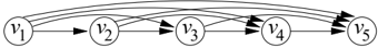
Figure 1 illustrates the causal graph of a planning problem with two splitting state variables, v and w . The edge label v = 0 indicates that there are operators for changing the value of u that have v = 0 as a pre-condition. In other words, Q v 0 = { u, w } , the graph G v 0 = ( V, E v 0 ) excludes the two edges labeled v = 0, and V v 0 includes all state state variables,

since v is weakly connected to u and w connects to the remaining state variables. The set Q v 1 is empty since there are no operators for changing the value of a state variable other than v with v = 1 as a pre-condition. Consequently, V v 1 is empty as well. Figure 1(a) shows the resulting partition for v .

In the case of w , Q w 0 = { s } , G w 0 = ( V, E w 0 ) excludes the edge labeled w = 0, and V w 0 = { s } , since no other state variable is connected to s when the edge w = 0 is removed. Likewise, V w 1 = { t } . We use V w ∗ = V -V w 0 -V w 1 to denote the set of remaining state variables that belong neither to V w 0 nor to V w 1 . Figure 1(b) shows the resulting partition for w .

Lemma 3.5 For any splitting state variable v , if the two sets V v 0 and V v 1 are non-empty, v belongs neither to V v 0 nor to V v 1 .

Proof By contradiction. Assume that v belongs to V v 0 . Then v is weakly connected to some state variable of Q v 0 in the graph G v 0 = ( V, E v 0 ). But since E v 0 does not exclude edges between v and Q v 1 , any state variable in Q v 1 is weakly connected to the same state variable of Q v 0 in G v 0 . Consequently, state variables in Q v 1 belong to both V v 0 and V v 1 , which contradicts that v is splitting. The same reasoning holds to show that v does not belong to V v 1 .

Lemma 3.6 The value of a splitting state variable never needs to change more than twice on a valid plan.

Proof Assume Π is a valid plan that changes the value of a splitting state variable v at least three times. We show that we can reorder the operators of Π in such a way that the value of v does not need to change more than twice. We need to address three cases: v belongs to V v 0 (cf. Figure 1(a)), v belongs to V v 1 , or v belongs to V v ∗ (cf. Figure 1(b)).

If v belongs to V v 0 , it follows from Lemma 3.5 that V v 1 is empty. Consequently, no operator in the plan requires v = 1 as a pre-condition. Thus, we can safely remove all operators in Π that change the value of v , except possibly the last, which is needed in case goal ( v ) = 1. If v belongs to V v 1 , it follows from Lemma 3.5 that V v 0 is empty. Thus, no operator in the plan requires v = 0 as a pre-condition. The first operator in Π that changes the value of v is necessary to set v to 1. After that, we can safely remove all operators in Π that change the value of v , except the last in case goal ( v ) = 0. In both cases the resulting plan contains at most two operators changing the value of v .

If v belongs to V v ∗ , then the only edges between V v 0 , V v 1 , and V v ∗ are those from v ∈ V v ∗ to Q v 0 ⊆ V v 0 and Q v 1 ⊆ V v 1 . Let Π 0 , Π 1 , and Π ∗ be the subsequences of operators in Π that affect state variables in V v 0 , V v 1 , and V v ∗ , respectively. Write Π ∗ = 〈 Π ′ ∗ , a v 1 , Π ′′ ∗ 〉 , where a v 1 is the last operator in Π ∗ that changes the value of v from 0 to 1. We claim that the reordering 〈 Π 0 , Π ′ ∗ , a v 1 , Π 1 , Π ′′ ∗ 〉 of plan Π is still valid. Indeed, the operators of Π 0 only require v = 0, which holds in the initial state, and the operators of Π 1 only require v = 1, which holds due to the operator a v 1 . Note that all operators changing the value of v in Π ′ ∗ can be safely removed since the value v = 1 is never needed as a pre-condition to change the value of a state variable in V v ∗ . The result is a valid plan that changes the value of v at most twice (its value may be reset to 0 by Π ′′ ∗ ).

Variable	Operators	V v i 0	V v i 1
v 1	a v 1 1 = 〈 ( v 1 = 0); ( v 1 = 1) 〉 a v 1 0 = 〈 ( v 1 = 1); ( v 1 = 0) 〉	V	V
v 2	a v 2 1 = 〈 ( v 1 = 1 , v 2 = 0); ( v 2 = 1) 〉	∅	V
v 3	a v 3 1 = 〈 ( v 1 = 0 , v 2 = 1 , v 3 = 0); ( v 3 = 1) 〉	{ v 4 , v 5 } V -{ v 4 }	{ v 6 , v 7 , v 8 } ∅
v 4 v 5	a v 5 1 = 〈 ( v 3 = 0 , v 4 = 0 , v 5 = 0); ( v 5 = 1) 〉	∅	∅
v 6	a v 6 1 = 〈 ( v 3 = 1 , v 6 = 0); ( v 6 = 1) 〉 a v 6 0 = 〈 ( v 3 = 1 , v 6 = 1); ( v 6 = 0) 〉	V	V
v 7	a v 7 1 = 〈 ( v 6 = 1 , v 7 = 0); ( v 7 = 1) 〉	∅	V
v 8	a v 8 = 〈 ( v 6 = 0 , v 7 = 1 , v 8 = 0); ( v 8 = 1) 〉	∅	∅

1

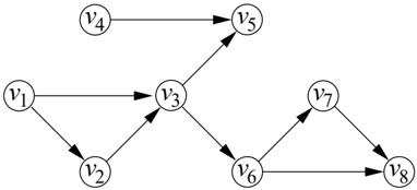
Figure 2: Causal graph of the example planning problem.

The previous lemma, which holds for splitting state variables in general, provides some additional insight into how to solve a planning problem with a splitting state variable v . First, try to achieve the goal state for state variables in V v 0 while the value of v is 0, as in the initial state. Then, set the value of v to 1 and try to achieve the goal state for state variables in V v 1 . Finally, if goal ( v ) = 0, reset the value of v to 0.

3.1 Example

We illustrate the class 3S using an example planning problem. The set of state variables is V = { v 1 , . . . , v 8 } . Since the planning problem is in normal form, the initial state is init ( v i ) = 0 for each v i ∈ V . The goal state is defined by goal = ( v 5 = 1 , v 8 = 1), and the operators in A are listed in Table 1. Figure 2 shows the causal graph ( V, E ) of the planning problem. From the operators it is easy to verify that v 4 is static and that v 1 and v 6 are symmetrically reversible. For the planning problem to be in 3S , the remaining state variables have to be splitting. Table 1 lists the two sets V v i 0 and V v i 1 for each state variable v i ∈ V to show that indeed, V v i 0 ∩ V v i 1 = ∅ for each of the state variables in the set { v 2 , v 3 , v 5 , v 7 , v 8 } .

4. Plan Generation for 3S

In this section, we present a polynomial-time algorithm for plan generation in 3S . The algorithm produces a solution to any instance of 3S in the form of a system of macros. The idea is to construct unary macros that each change the value of a single state variable. The macros may change the values of other state variables during execution, but always reset them before terminating. Once the macros have been generated, the goal can be achieved one state variable at a time. We show that the algorithm generates a valid plan if and only if one exists.

We begin by defining macros as we use them in the paper. Next, we describe the algorithm in pseudo-code (Figures 3, 4, and 5) and prove its correctness. To facilitate reading we have moved a straightforward but involving proof to the appendix. Following the description of the algorithm we analyze the complexity of all steps involved. In what follows, we assume that 3S planning problems are in normal form as defined in the previous section.

4.1 Macros

A macro-operator, or macro for short, is an ordered sequence of operators viewed as a unit. Each operator in the sequence has to respect the pre-conditions of operators that follow it, so that no pre-condition of any operator in the sequence is violated. Applying a macro is equivalent to applying all operators in the sequence in the given order. Semantically, a macro is equivalent to a standard operator in that it has a pre-condition and a postcondition, unambiguously induced by the pre- and post-conditions of the operators in its sequence.

Since macros are functionally operators, the operator sequence associated with a macro can include other macros, as long as this does not create a circular definition. Consequently, it is possible to create hierarchies of macros in which the operator sequences of macros on one level include macros on the level below. The solution to a planning problem can itself be viewed as a macro which sits at the top of the hierarchy.

To define macros we first introduce the concept of induced pre- and post-conditions of operator sequences. If Π = 〈 a 1 , . . . , a k 〉 is an operator sequence, we write Π i , 1 ≤ i ≤ k , to denote the subsequence 〈 a 1 , . . . , a i 〉 .

Definition 4.1 An operator sequence Π = 〈 a 1 , . . . , a k 〉 induces a pre-condition pre (Π) = pre ( a k ) ⊕···⊕ pre ( a 1 ) and a post-condition post (Π) = post ( a 1 ) ⊕···⊕ post ( a k ) . In addition, the operator sequence is well-defined if and only if ( pre (Π i -1 ) ⊕ post (Π i -1 )) /triangleinv pre ( a i ) for each 1 < i ≤ k .

In what follows, we assume that P = ( V, init, goal, A ) is a planning problem such that V post ( a ) ⊆ V pre ( a ) for each operator a ∈ A , and that Π = 〈 a 1 , . . . , a k 〉 is an operator sequence.

Lemma 4.2 For each planning problem P of this type and each Π , V post (Π) ⊆ V pre (Π) .

Proof A direct consequence of the definitions V pre (Π) = V pre ( a 1 ) ∪·· ·∪ V pre ( a k ) and V post (Π) = V post ( a 1 ) ∪ · · · ∪ V post ( a k ) .

Lemma 4.3 The operator sequence Π is applicable in state s if and only if Π is well-defined and s /triangleinv pre (Π) . The state s k resulting from the application of Π to s is s k = s ⊕ post (Π) .

Proof By induction on k . The result clearly holds for k = 1. For k > 1, note that pre (Π) = pre ( a k ) ⊕ pre (Π k -1 ), post (Π) = post (Π k -1 ) ⊕ post ( a k ), and Π is well-defined if and only if Π k -1 is well-defined and ( pre (Π k -1 ) ⊕ post (Π k -1 )) /triangleinv pre ( a k ).

By hypothesis of induction the state s k -1 resulting from the application of Π k -1 to s is s k -1 = s ⊕ post (Π k -1 ). It follows that s k = s k -1 ⊕ post ( a k ) = s ⊕ post (Π).

Assume Π is applicable in state s . This means that Π k -1 is applicable in s and that a k is applicable in s k -1 = s ⊕ post (Π k -1 ). By hypothesis of induction, the former implies that s /triangleinv pre (Π k -1 ) and Π k -1 is well-defined, and the latter that ( s ⊕ post (Π k -1 )) /triangleinv pre ( a k ). This last condition implies that ( pre (Π k -1 ) ⊕ post (Π k -1 )) /triangleinv pre ( a k ) if we use that pre (Π k -1 ) /subsetsqequal s , which is a consequence of s /triangleinv pre (Π k -1 ) and s being a total state. Finally, we deduce s /triangleinv ( pre ( a k ) ⊕ pre (Π k -1 )) from s /triangleinv pre (Π k -1 ) and ( s ⊕ post (Π k -1 )) /triangleinv pre ( a k ), by using that V post (Π k -1 ) ⊆ V pre (Π k -1 ) . It follows that Π is well-defined and that s /triangleinv pre (Π).

Conversely, assume that Π is well-defined and s /triangleinv pre (Π). This implies that Π k -1 is well-defined and s /triangleinv pre (Π k -1 ), so by hypothesis of induction, Π k -1 is applicable in state s . It remains to show that a k is applicable in state s k -1 , that is, ( s ⊕ post (Π k -1 )) /triangleinv pre ( a k ). From ( pre (Π k -1 ) ⊕ post (Π k -1 )) /triangleinv pre ( a k ) it follows that post (Π k -1 ) /triangleinv pre ( a k ). The fact that s /triangleinv ( pre ( a k ) ⊕ pre (Π k -1 )) and V post (Π k -1 ) ⊆ V pre (Π k -1 ) completes the proof.

Since macros have induced pre- and post-conditions, Lemmas 4.2 and 4.3 trivially extend to the case for which the operator sequence Π includes macros. Now we are ready to introduce our definition of macros:

Definition 4.4 A macro m is a sequence Π = 〈 a 1 , . . . , a k 〉 of operators and other macros that induces a pre-condition pre ( m ) = pre (Π) and a post-condition post ( m ) = post (Π) -pre (Π) . The macro is well-defined if and only if no circular definitions occur and Π is well-defined.

To make macros consistent with standard operators, the induced post-condition should only include state variables whose values are indeed changed by the macro, which is achieved by computing the difference between post (Π) and pre (Π). In particular, it holds that for a 3S planning problem in normal form, derived macros satisfy the second condition of normal form, namely that post ( m ) = ( v = x ), x ∈ { 0 , 1 } , implies pre ( m )( v ) = 1 -x .

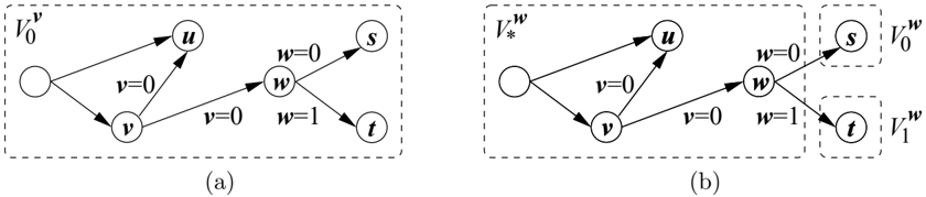
Definition 4.5 Let Anc v be the set of ancestors of a state variable v in a 3S planning problem. We define the partial state pre v on V pre v = Anc v as

1. pre v ( u ) = 1 if u ∈ Anc v is splitting and v ∈ V u 1 ,
2. pre v ( u ) = 0 otherwise.

Definition 4.6 A macro m is a 3S -macro if it is well-defined and, for x ∈ { 0 , 1 } , post ( m ) = ( v = x ) and pre ( m ) /subsetsqequal pre v ⊕ ( v = 1 -x ) .

Table 2: Macros generated by the algorithm in the example planning problem.

Macro	Sequence	Pre-condition	Post-condition
m v 1 1	〈 a v 1 1 〉	( v 1 = 0)	( v 1 = 1)
m v 1 0	〈 a v 1 0 〉	( v 1 = 1)	( v 1 = 0)
m v 2 1	〈 m v 1 1 ,a v 2 1 ,m v 1 0 〉	( v 1 = 0 , v 2 = 0)	( v 2 = 1)
m v 3 1	〈 a v 3 1 〉	( v 1 = 0 , v 2 = 1 , v 3 = 0)	( v 3 = 1)
m v 5 1	〈 a v 5 1 〉	( v 3 = 0 , v 4 = 0 , v 5 = 0)	( v 5 = 1)
m v 6 1	〈 a v 6 1 〉	( v 3 = 1 , v 6 = 0)	( v 6 = 1)
m v 6 0	〈 a v 6 0 〉	( v 3 = 1 , v 6 = 1)	( v 6 = 0)
m v 7 1	〈 m v 6 1 ,a v 7 1 ,m v 6 0 〉	( v 3 = 1 , v 6 = 0 , v 7 = 0)	( v 7 = 1)
m v 8 1	〈 a v 8 1 〉	( v 3 = 1 , v 6 = 0 , v 7 = 1 , v 8 = 0)	( v 8 = 1)

The algorithm we present only generates 3S -macros. In fact, it generates at most one macro m = m v x with post ( m ) = ( v = x ) for each state variable v and value x ∈ { 0 , 1 } . To illustrate the idea of 3S -macros and give a flavor of the algorithm, Table 2 lists the macros generated by the algorithm in the example 3S planning problem from the previous section.

We claim that each macro is a 3S -macro. For example, the operator sequence 〈 a v 6 1 〉 induces a pre-condition ( v 3 = 1 , v 6 = 0) and a post-condition ( v 3 = 1 , v 6 = 0) ⊕ ( v 6 = 1) = ( v 3 = 1 , v 6 = 1). Thus, the macro m v 6 1 induces a pre-condition pre ( m v 6 1 ) = ( v 3 = 1 , v 6 = 0) and a post-condition post ( m v 6 1 ) = ( v 3 = 1 , v 6 = 1) -( v 3 = 1 , v 6 = 0) = ( v 6 = 1). Since v 2 and v 3 are splitting and since v 6 ∈ V v 2 1 and v 6 ∈ V v 3 1 , it follows that pre v 6 ⊕ ( v 6 = 0) = ( v 1 = 0 , v 2 = 1 , v 3 = 1 , v 6 = 0), so pre ( m v 6 1 ) = ( v 3 = 1 , v 6 = 0) /subsetsqequal pre v 6 ⊕ ( v 6 = 0).

The macros can be combined to produce a solution to the planning problem. The idea is to identify each state variable v such that goal ( v ) = 1 and append the macro m v 1 to the solution plan. In the example, this results in the operator sequence 〈 m v 5 1 , m v 8 1 〉 . However, the pre-condition of m v 8 1 specifies v 3 = 1 and v 7 = 1, which makes it necessary to insert m v 3 1 and m v 7 1 before m v 8 1 . In addition, the pre-condition of m v 3 1 specifies v 2 = 1, which makes it necessary to insert m v 2 1 before m v 3 1 , resulting in the final plan 〈 m v 5 1 , m v 2 1 , m v 3 1 , m v 7 1 , m v 8 1 〉 . Note that the order of the macros matter; m v 5 1 requires v 3 to be 0 while m v 8 1 requires v 3 to be 1. For a splitting state variable v , the goal state should be achieved for state variables in V v 0 before the value of v is set to 1. We can expand the solution plan so that it consists solely of operators in A . In our example, this results in the operator sequence 〈 a v 5 1 , a v 1 1 , a v 2 1 , a v 1 0 , a v 3 1 , a v 6 1 , a v 7 1 , a v 6 0 , a v 8 1 〉 . In this case, the algorithm generates an optimal plan, although this is not true in general.

4.2 Description of the Algorithm

We proceed by providing a detailed description of the algorithm for plan generation in 3S . We first describe the subroutine for generating a unary macro that sets the value of a state variable v to x . This algorithm, which we call GenerateMacro , is described in Figure 3. The algorithm takes as input a planning problem P , a state variable v , a value x (either 0

1 function GenerateMacro ( P , v , x , M ) 2 for each a ∈ A such that post ( a )( v ) = x do 3 S 0 ← S 1 ←〈〉 4 satisfy ← true 5 U ←{ u ∈ V pre ( a ) -{ v } | pre ( a )( u ) = 1 } 6 for each u ∈ U in increasing topological order do 7 if u is static or m u 1 / ∈ M then 8 satisfy ← false 9 else if u is not splitting and m u 0 ∈ M and m u 1 ∈ M then 10 S 0 ←〈 S 0 , m u 0 〉 11 S 1 ←〈 m u 1 , S 1 〉 12 if satisfy then 13 return 〈 S 1 , a, S 0 〉 14 return fail

or 1), and a set of macros M for v 's ancestors in the causal graph. Prior to executing the algorithm, we perform a topological sort of the state variables. We assume that, for each v ∈ V and x ∈ { 0 , 1 } , M contains at most one macro m v x such that post ( m v x ) = ( v = x ). In the algorithm, we use the notation m v x ∈ M to test whether or not M contains m v x .

For each operator a ∈ A that sets the value of v to x , the algorithm determines whether it is possible to satisfy its pre-condition pre ( a ) starting from the initial state. To do this, the algorithm finds the set U of state variables to which pre ( a ) assigns 1 (the values of all other state variables already satisfy pre ( a ) in the initial state). The algorithm constructs two sequences of operators, S 0 and S 1 , by going through the state variables of U in increasing topological order. If S is an operator sequence, we use 〈 S, o 〉 as shorthand to denote an operator sequence of length | S | +1 consisting of all operators of S followed by o , which can be either an operator or a macro. If it is possible to satisfy the pre-condition pre ( a ) of some operator a ∈ A , the algorithm returns the macro 〈 S 1 , a, S 0 〉 . Otherwise, it returns fail .

Lemma 4.7 If v is symmetrically reversible and GenerateMacro ( P , v , 1, M ) successfully generates a macro, so does GenerateMacro ( P , v , 0, M ).

Proof Assume that GenerateMacro ( P , v , 1, M ) successfully returns the macro 〈 S 1 , a, S 0 〉 for some operator a ∈ A such that post ( a ) = 1. From the definition of symmetrically reversible it follows that there exists an operator a ′ ∈ A such that post ( a ′ ) = 0 and pre ( a ′ ) | V - { v } = pre ( a ) | V - { v } . Thus, the set U is identical for a and a ′ . As a consequence, the values of S 0 , S 1 , and satisfy are the same after the loop, which means that GenerateMacro ( P , v , 0, M ) returns the macro 〈 S 1 , a ′ , S 0 〉 for a ′ . Note that GenerateMacro ( P , v , 0, M ) may return another macro if it goes through the operators of A in a different order; however, it is guaranteed to successfully return a macro.

/negationslash

Theorem 4.8 If the macros in M are 3S -macros and GenerateMacro ( P , v , x , M ) generates a macro m v x = fail , then m v x is a 3S -macro.

/negationslash

/negationslash

/negationslash

/negationslash

1 function Macro-3S ( P ) 2 M ←∅ 3 for each v ∈ V in increasing topological order do 4 m v 1 ← GenerateMacro ( P , v , 1, M ) 5 m v 0 ← GenerateMacro ( P , v , 0, M ) 6 if m v 1 = fail and m v 0 = fail then 7 M ← M ∪{ m v 1 , m v 0 } 8 else if m v 1 = fail and goal ( v ) = 0 then 9 M ← M ∪{ m v 1 } 10 return GeneratePlan ( P , V , M )

The proof of Theorem 4.8 appears in Appendix A.

Next, we describe the algorithm for plan generation in 3S , which we call Macro-3S . Figure 4 shows pseudocode for Macro-3S . The algorithm goes through the state variables in increasing topological order and attempts to generate two macros for each state variable v , m v 1 and m v 0 . If both macros are successfully generated, they are added to the current set of macros M . If only m v 1 is generated and the goal state does not assign 0 to v , the algorithm adds m v 1 to M . Finally, the algorithm generates a plan using the subroutine GeneratePlan , which we describe later.

Lemma 4.9 Let P be a 3S planning problem and let v ∈ V be a state variable. If there exists a valid plan for solving P that sets v to 1, Macro-3S ( P ) adds the macro m v 1 to M . If, in addition, the plan resets v to 0, Macro-3S ( P ) adds m v 0 to M .

/negationslash

Proof First note that if m v 1 and m v 0 are generated, Macro-3S ( P ) adds them both to M . If m v 1 is generated but not m v 0 , Macro-3S ( P ) adds m v 1 to M unless goal ( v ) = 0. However, goal ( v ) = 0 contradicts the fact that there is a valid plan for solving P that sets v to 1 without resetting it to 0. It remains to show that GenerateMacro ( P , v , 1, M ) always generates m v 1 = fail and that GenerateMacro ( P , v , 0, M ) always generates m v 0 = fail if the plan resets v to 0.

/negationslash

/negationslash

A plan for solving P that sets v to 1 has to contain an operator a ∈ A such that post ( a )( v ) = 1. If the plan also resets v to 0, it has to contain an operator a ′ ∈ A such that post ( a ′ )( v ) = 0. We show that GenerateMacro ( P , v , 1, M ) successfully generates m v 1 = fail if a is the operator selected on line 2. Note that the algorithm may return another macro if it selects another operator before a ; however, if it always generates a macro for a , it is guaranteed to successfully return a macro m v 1 = fail . The same is true for m v 0 and a ′ .

/negationslash

We prove the lemma by induction on state variables v . If v has no ancestors in the causal graph, the set U is empty by default. Thus, satisfy is never set to false and GenerateMacro ( P , v , 1, M ) successfully returns the macro m v 1 = 〈 a 〉 for a . If a ′ exists, GenerateMacro ( P , v , 0, M ) successfully returns m v 0 = 〈 a ′ 〉 for a ′ .

If v has ancestors in the causal graph, let U = { u ∈ V pre ( a ) - { v } | pre ( a )( u ) = 1 } . Since the plan contains a it has to set each u ∈ U to 1. By hypothesis of induction, Macro-3S ( P ) adds m u 1 to M for each u ∈ U . As a consequence, satisfy is never set to

1 function GeneratePlan ( P , W , M ) 2 if | W | = 0 then 3 return 〈〉 4 v ← first variable in topological order present in W 5 if v is splitting then 6 Π v 0 ← Generate-Plan ( P , W ∩ ( V v 0 -{ v } ), M ) 7 Π v 1 ← Generate-Plan ( P , W ∩ ( V v 1 -{ v } ), M ) 8 Π v ∗ ← Generate-Plan ( P , W ∩ ( V -V v 0 -V v 1 -{ v } ), M ) 9 if Π v 0 = fail or Π v 1 = fail or Π v ∗ = fail or ( goal ( v ) = 1 and m v 1 / ∈ M ) then 10 return fail 11 else if m v 1 / ∈ M then return 〈 Π v ∗ , Π v 0 , Π v 1 〉 12 else if goal ( v ) = 0 then return 〈 Π v ∗ , Π v 0 , m v 1 , Π v 1 , m v 0 〉 13 else return 〈 Π v ∗ , Π v 0 , m v 1 , Π v 1 〉 14 Π ← Generate-Plan ( P , W -{ v } , M ) 15 if Π = fail or ( goal ( v ) = 1 and m v 1 / ∈ M ) then return fail 16 else if goal ( v ) = 1 then return 〈 Π , m v 1 〉 17 else return Π

false and thus, GenerateMacro ( P , v , 1, M ) successfully returns m v 1 for a . If a ′ exists, let W = { w ∈ V pre ( a ′ ) - { v } | pre ( a ′ )( w ) = 1 } . If the plan contains a ′ , it has to set each w ∈ W to 1. By hypothesis of induction, Macro-3S ( P ) adds m w 1 to M for each w ∈ W and consequently, GenerateMacro ( P , v , 0, M ) successfully returns m v 0 for a ′ .

Finally, we describe the subroutine GeneratePlan ( P , W , M ) for generating the final plan given a planning problem P , a set of state variables W and a set of macros M . If the set of state variables is empty, GeneratePlan ( P , W , M ) returns an empty operator sequence. Otherwise, it finds the state variable v ∈ W that comes first in topological order. If v is splitting, the algorithm separates W into the three sets described by V v 0 , V v 1 , and V v ∗ = V -V v 0 -V v 1 . The algorithm recursively generates plans for the three sets and if necessary, inserts m v 1 between V v 0 and V v 1 in the final plan. If this is not the case, the algorithm recursively generates a plan for W -{ v } . If goal ( v ) = 1 and m v 1 , the algorithm appends m v 1 to the end of the resulting plan.

Lemma 4.10 Let Π W be the plan generated by GeneratePlan ( P , W , M ), let v be the first state variable in topological order present in W , and let Π V = 〈 Π a , Π W , Π b 〉 be the final plan generated by Macro-3S ( P ). If m v 1 ∈ M it follows that ( pre (Π a ) ⊕ post (Π a )) /triangleinv pre ( m v 1 ) .

Proof We determine the content of the operator sequence Π a that precedes Π W in the final plan by inspection. Note that the call GeneratePlan ( P , W , M ) has to be nested within a sequence of recursive calls to GeneratePlan starting with GeneratePlan ( P , V , M ). Let Z be the set of state variables such that each u ∈ Z was the first state variable in topological order for some call to GeneratePlan prior to GeneratePlan ( P , W , M ). Each u ∈ Z has to correspond to a call to GeneratePlan with some set of state variables U such that W ⊂ U . If u is not splitting, u does not contribute to Π a since the only

possible addition of a macro to the plan on line 16 places the macro m u 1 at the end of the plan generated recursively.

Assume that u ∈ Z is a splitting state variable. We have three cases: W ⊆ V u 0 , W ⊆ V u 1 , and W ⊆ V u ∗ = V -V u 0 -V u 1 . If W ⊆ V u ∗ , u does not contribute to Π a since it never places macros before Π u ∗ . If W ⊆ V u 0 , the plan Π u ∗ is part of Π a since it precedes Π u 0 on lines 11, 12, and 13. If W ⊆ V u 1 , the plans Π u ∗ and Π u 0 are part of Π a since they both precede Π u 1 in all cases. If m u 1 ∈ M , the macro m u 1 is also part of Π a since it precedes Π u 1 on lines 12 and 13. No other macros are part of Π a .

Since the macros in M are unary, the plan generated by GeneratePlan ( P , U , M ) only changes the values of state variables in U . For a splitting state variable u , there are no edges from V u ∗ -{ u } to V u 0 , from V u ∗ -{ u } to V u 1 , or from V u 0 to V u 1 . It follows that the plan Π u ∗ does not change the value of any state variable that appears in the pre-condition of a macro in Π u 0 . The same holds for Π u ∗ with respect to Π u 1 and for Π u 0 with respect to Π u 1 . Thus, the only macro in Π a that changes the value of a splitting state variable u ∈ Anc v is m u 1 in case W ⊆ V u 1 .

Recall that pre v is defined on Anc v and assigns 1 to u if and only if u is splitting and v ∈ V u 1 . For all other ancestors of v , the value 0 holds in the initial state and is not altered by Π a . If u is splitting and v ∈ V u 1 , it follows from the definition of 3S -macros that pre ( m v 1 )( u ) = 1 or pre ( m v 1 )( u ) = ⊥ . If pre ( m v 1 )( u ) = 1, it is correct to append m u 1 before m v 1 to satisfy pre ( m v 1 )( u ). If m u 1 / ∈ M it follows that u / ∈ V pre ( m v 1 ) , since pre ( m v 1 )( u ) = 1 would have caused GenerateMacro ( P , v , 1, M ) to set satisfy to false on line 8. Thus, the pre-condition pre ( m v 1 ) of m v 1 agrees with pre (Π a ) ⊕ post (Π a ) on the value of each state variable, which means that the two partial states match.

Lemma 4.11 GeneratePlan ( P , V , M ) generates a well-defined plan.

Proof Note that for each state variable v ∈ V , GeneratePlan ( P , W , M ) is called precisely once such that v is the first state variable in topological order. From Lemma 4.10 it follows that ( pre (Π a ) ⊕ post (Π a )) /triangleinv pre ( m v 1 ), where Π a is the plan that precedes Π W in the final plan. Since v is the first state variable in topological order in W , the plans Π v 0 , Π v 1 , Π v ∗ , and Π, recursively generated by GeneratePlan , do not change the value of any state variable in pre ( m v 1 ). It follows that m v 1 is applicable following 〈 Π a , Π v ∗ , Π v 0 〉 or 〈 Π a , Π 〉 . Since m v 1 only changes the value of v , m v 0 is applicable following 〈 Π a , Π v ∗ , Π v 0 , m v 1 , Π v 1 〉 .

Theorem 4.12 Macro-3S ( P ) generates a valid plan for solving a planning problem in 3S if and only if one exists.

Proof GeneratePlan ( P , V , M ) returns fail if and only if there exists a state variable v ∈ V such that goal ( v ) = 1 and m v 1 / ∈ M . From Lemma 4.9 it follows that there does not exist a valid plan for solving P that sets v to 1. Consequently, there does not exist a plan for solving P . Otherwise, GeneratePlan ( P , V , M ) returns a well-defined plan due to Lemma 4.11. Since the plan sets to 1 each state variable v such that goal ( v ) = 1 and resets to 0 each state variable v such that goal ( v ) = 0, the plan is a valid plan for solving the planning problem.

4.3 Examples

We illustrate the algorithm on an example introduced by Jonsson and B¨ ackstr¨ om (1998) to show that there are instances of 3S with exponentially sized minimal solutions. Let P n = 〈 V, init, goal, A 〉 be a planning problem defined by a natural number n , V = { v 1 , . . . , v n } , and a goal state defined by V goal = V , goal ( v i ) = 0 for each v i ∈ { v 1 , . . . , v n -1 } , and goal ( v n ) = 1. For each state variable v i ∈ V , there are two operators in A :

In other words, each state variable is symmetrically reversible. The causal graph of the planning problem P 5 is shown in Figure 6. Note that for each state variable v i ∈ { v 1 , . . . , v n -2 } , pre ( a v i +1 1 )( v i ) = 1 and pre ( a v i +2 1 )( v i ) = 0, so v i +1 ∈ Q v i 1 and v i +2 ∈ Q v i 0 . Since there is an edge in the causal graph between v i +1 and v i +2 , no state variable in { v 1 , . . . , v n -2 } is splitting. On the other hand, v n -1 and v n are splitting since V v n -1 0 = ∅ and V v n 0 = V v n 1 = ∅ . B¨ ackstr¨ om and Nebel (1995) showed that the length of the shortest plan solving P n is 2 n -1, i.e., exponential in the number of state variables.

For each state variable v i ∈ { v 1 , . . . , v n -1 } , our algorithm generates two macros m v i 1 and m v i 0 . There is a single operator, a v i 1 , that changes the value of v i from 0 to 1. pre ( a v i 1 ) only assigns 1 to v i -1 , so U = { v i -1 } . Since v i -1 is not splitting, m v i 1 is defined as m v i 1 = 〈 m v i -1 1 , a v i 1 , m v i -1 0 〉 . Similarly, m v i 0 is defined as m v i 0 = 〈 m v i -1 1 , a v i 0 , m v i -1 0 〉 . For state variable v n , U = { v n -1 } , which is splitting, so m v n 1 is defined as m v n 1 = 〈 a v n 1 〉 .

To generate the final plan, the algorithm goes through the state variables in topological order. For state variables v 1 through v n -2 , the algorithm does nothing, since these state variables are not splitting and their goal state is not 1. For state variable v n -1 , the algorithm recursively generates the plan for v n , which is 〈 m v n 1 〉 since goal ( v n ) = 1. Since goal ( v n -1 ) = 0, the algorithm inserts m v n -1 1 before m v n 1 to satisfy its pre-condition v n -1 = 1 and m v n -1 0 after m v n 1 to achieve the goal state goal ( v n -1 ) = 0. Thus, the final plan is 〈 m v n -1 1 , m v n 1 , m v n -1 0 〉 . If we expand the plan, we end up with a sequence of 2 n -1 operators. However, no individual macro has operator sequence length greater than 3. Together, the macros recursively specify a complete solution to the planning problem.

We also demonstrate that there are planning problems in 3S with polynomial length solutions for which our algorithm may generate exponential length solutions. To do this, we modify the planning problem P n by letting goal ( v i ) = 1 for each v i ∈ V . In addition, for each state variable v i ∈ V , we add two operators to A :

We also add an operator c v n 1 = 〈 ( v n -1 = 0 , v n = 0); ( v n = 1) 〉 to A . As a consequence, state variables in { v 1 , . . . , v n -2 } are still symmetrically reversible but not splitting. v n -1 is also symmetrically reversible but no longer splitting, since pre ( a v n 1 )( v n -1 ) = 1 and pre ( c v n 1 )( v n -1 ) = 0 implies that v n ∈ V v n -1 0 ∩ V v n -1 1 . v n is still splitting since V v n 0 = V v n 1 = ∅ . Assume that GenerateMacro ( P , v i , x , M ) always selects b v i x first. As a consequence, for each state variable v i ∈ V and each x ∈ { 0 , 1 } , GenerateMacro ( P , v i , x , M ) generates the macro m v i x = 〈 m v i -1 1 , . . . , m v 1 1 , b v i x , m v 1 0 , . . . , m v i -1 0 〉 .

Let L i be the length of the plan represented by m v i x , x ∈ { 0 , 1 } . From the definition of m v i x above we have that L i = 2( L 1 + . . . + L i -1 ) + 1. We show by induction that L i = 3 i -1 . The length of any macro for v 1 is L 1 = 1 = 3 0 . For i > 1,

To generate the final plan the algorithm has to change the value of each state variable from 0 to 1, so the total length of the plan is L = L 1 + . . . + L n = 3 0 + . . . + 3 n -1 = (3 n -1) / 2. However, there exists a plan of length n that solves the planning problem, namely 〈 b v 1 1 , . . . , b v n 1 〉 .

4.4 Complexity

In this section we prove that the complexity of our algorithm is polynomial. To do this we analyze each step of the algorithm separately. A summary of the complexity result for each step of the algorithm is given below. Note that the number of edges | E | in the causal graph is O ( | A || V | ), since each operator may introduce O ( | V | ) edges. The complexity result O ( | V | + | E | ) = O ( | A || V | ) for topological sort follows from Cormen, Leiserson, Rivest, and Stein (1990).

Constructing the causal graph G = ( V,E	O ( | A || V | )	Lemma 4.13
Calculating V v 1 and V v 0 for each v ∈ V	O ( | A || V | 2 )	Lemma 4.14
Performing a topological sort of G	O ( | A || V | )
GenerateMacro ( P , v , x , M )	O ( | A || V | )	Lemma 4.15
GeneratePlan ( P , V , M )	O ( | V | 2 )	Lemma 4.16
Macro-3S ( P )	O ( | A || V | 2 )	Theorem 4.17

Lemma 4.13 The complexity of constructing the causal graph G = ( V, E ) is O ( | A || V | ) .

Proof The causal graph consists of | V | nodes. For each operator a ∈ A and each state variable u ∈ V pre ( a ) , we should add an edge from u to the unique state variable v ∈ V post ( a ) . In the worst case, | V pre ( a ) | = O ( | V | ), in which case the complexity is O ( | A || V | ).

Lemma 4.14 The complexity of calculating the sets V v 0 and V v 1 for each state variable v ∈ V is O ( | A || V | 2 ) .

Proof For each state variable v ∈ V , we have to establish the sets Q v 0 and Q v 1 , which requires going through each operator a ∈ A in the worst case. Note that we are only interested in the pre-condition on v and the unique state variable in V post ( a ) , which means that we do not

need to go through each state variable in V pre ( a ) . Next, we have to construct the graph G v 0 . We can do this by copying the causal graph G , which takes time O ( | A || V | ), and removing the edges between v and Q v 0 -Q v 1 , which takes time O ( | V | ).

Finally, to construct the set V v 0 we should find each state variable that is weakly connected to some state variable u ∈ Q v 0 in the graph G v 0 . For each state variable u ∈ Q v 0 , performing an undirected search starting at u takes time O ( | A || V | ). Once we have performed search starting at u , we only need to search from state variables in Q v 0 that were not reached during the search. This way, the total complexity of the search does not exceed O ( | A || V | ). The case for constructing V v 1 is identical. Since we have to perform the same procedure for each state variable v ∈ V , the total complexity of this step is O ( | A || V | 2 ).

Lemma 4.15 The complexity of GenerateMacro ( P , v , x , M ) is O ( | A || V | ) .

Proof For each operator a ∈ A , GenerateMacro ( P , v , x , M ) needs to check whether post ( a )( v ) = x . In the worst case, | U | = O ( | V | ), in which case the complexity of the algorithm is O ( | A || V | ).

Lemma 4.16 The complexity of GeneratePlan ( P , V , M ) is O ( | V | 2 ) .

Proof Note that for each state variable v ∈ V , GeneratePlan ( P , V , M ) is called recursively exactly once such that v is the first variable in topological order. In other words, GeneratePlan ( P , V , M ) is called exactly | V | times. GeneratePlan ( P , V , M ) contains only constant operations except the intersection and difference between sets on lines 6-8. Since intersection and set difference can be done in time O ( | V | ), the total complexity of GeneratePlan ( P , V , M ) is O ( | V | 2 ).

Theorem 4.17 The complexity of Macro-3S ( P ) is O ( | A || V | 2 ) .

Proof Prior to executing Macro-3S ( P ), it is necessary to construct the causal graph G , find the sets V v 0 and V v 1 for each state variable v ∈ V , and perform a topological sort of G . We have shown that these steps take time O ( | A || V | 2 ). For each state variable v ∈ V , Macro-3S ( P ) calls GenerateMacro ( P , v , x , M ) twice. From Lemma 4.15 it follows that this step takes time O (2 | V || A || V | ) = O ( | A || V | 2 ). Finally, Macro-3S ( P ) calls GeneratePlan ( P , V , M ), which takes time O ( | V | 2 ) due to Lemma 4.16. It follows that the complexity of Macro-3S ( P ) is O ( | A || V | 2 ).

We conjecture that it is possible to improve the above complexity result for Macro3S ( P ) to O ( | A || V | ). However, the proof seems somewhat complex, and our main objective is not to devise an algorithm that is as efficient as possible. Rather, we are interested in establishing that our algorithm is polynomial, which follows from Theorem 4.17.

4.5 Plan Length

In this section we study the length of the plans generated by the given algorithm. To begin with, we derive a general bound on the length of such plans. Then, we show how to compute the actual length of some particular plan without expanding its macros. We also present an algorithm that uses this computation to efficiently obtain the i -th action of the plan

from its macro form. We start by introducing the concept of depth of state variables in the causal graph.

Definition 4.18 The depth d ( v ) of a state variable v is the longest path from v to any other state variable in the causal graph.

Since the causal graph is acyclic for planning problems in 3S , the depth of each state variable is unique and can be computed in polynomial time. Also, it follows that at least one state variable has depth 0, i.e., no outgoing edges.

Definition 4.19 The depth d of a planning problem P in 3S equals the largest depth of any state variable v of P , i.e., d = max v ∈ V d ( v ) .

We characterize a planning problem based on the depth of each of its state variables. Let n = | V | be the number of state variables, and let c i denote the number of state variables with depth i . If the planning problem has depth d , it follows that c 0 + . . . + c d = n . As an example, consider the planning problem whose causal graph appears in Figure 2. For this planning problem, n = 8, d = 5, c 0 = 2, c 1 = 2, c 2 = 1, c 3 = 1, c 4 = 1, and c 5 = 1.

Lemma 4.20 Consider the values L i for i ∈ { 0 , . . . , d } defined by L d = 1 , and L i = 2( c i +1 L i +1 + c i +2 L i +2 + . . . + c d L d ) + 1 when i < d . The values L i are an upper bound on the length of macros generated by our algorithm for a state variable v with depth i .

Proof We prove it by a decreasing induction on the value of i . Assume v has depth i = d . It follows from Definition 4.18 that v has no incoming edges. Thus, an operator changing the value of v has no pre-condition on any state variable other than v , so L d = 1 is an upper bound, as stated.

Now, assume v has depth i < d , and that all L i + k for k > 0 are upper bounds on the length of the corresponding macros. Let a ∈ A be an operator that changes the value of v . From the definition of depth it follows that a cannot have a pre-condition on a state variable u with depth j ≤ i ; otherwise there would be an edge from u to v in the causal graph, causing the depth of u to be greater than i . Thus, in the worst case, a macro for v has to change the values of all state variables with depths larger than i , change the value of v , and reset the values of state variables at lower levels. It follows that L i = 2( c i +1 L i +1 + . . . + c d L d ) + 1 is an upper bound.

Theorem 4.21 The upper bounds L i of Lemma 4.20 satisfy L i = Π d j = i +1 (1 + 2 c j ) .

Proof Note that

The result easily follows by induction.

/negationslash

Now we can obtain an upper bound L on the total length of the plan. In the worst case, the goal state assigns a different value to each state variable than the initial state, i.e., goal ( v ) = init ( v ) for each v ∈ V . To achieve the goal state the algorithm applies one macro per state variable. Hence

The previous bound depends on the distribution of the variables on depths according to the causal graph. To obtain a general bound that does not depend on the depths of the variables we first find which distribution maximizes the upper bound L .

Lemma 4.22 The upper bound L = 1 2 ∏ d j =0 (1+2 c j ) -1 2 on planning problems on n variables and depth d is maximized when all c i are equal, that is, c i = n/ ( d +1) .

Proof Note that c i > 0 for all i , and that c 0 + · · · + c d = n . The result follows from a direct application of the well known AM-GM (arithmetic mean-geometric mean) inequality, which states that the arithmetic mean of positive values x i is greater or equal than its geometric mean, with equality only when all x i are the same. This implies that the product of positive factors x i = (1 + 2 c i ) with fixed sum A = ∑ d j =0 x j = 2 n + d is maximized when all are equal, that is, c i = n/ ( d +1).

Theorem 4.23 The length of a plan generated by the algorithm for a planning problem in 3S with n state variables and depth d is at most ((1 + 2 n/ ( d +1)) d +1 -1) / 2 .

Proof This is a direct consequence of Lemma 4.22. Since c 0 , . . . , c d are discrete, it may not be possible to set c 0 = . . . = c d = n/ ( d +1). Nevertheless, ((1 + 2 n/ ( d +1)) d +1 -1) / 2 is an upper bound on L in this case.

Observe that the bound established in Theorem 4.23 is an increasing function of d . This implies that for a given d , the bound also applies to planning problems in 3S with depth smaller than d . As a consequence, if the depth of a planning problem in 3S is bounded from above by d , our algorithm generates a solution plan for the planning problem with polynomial length O ( n d +1 ). Since the complexity of executing a plan is proportional to the plan length, we can use the depth d to define tractable complexity classes of planning problems in 3S with respect to plan execution.

Theorem 4.24 The length of a plan generated by the algorithm for a planning problem in 3S with n state variables is at most (3 n -1) / 2 .

Proof In the worst case, the depth d of a planning problem is n -1. It follows from Theorem 4.23 that the length of a plan is at most ((1 + 2 n/n ) n -1) / 2 = (3 n -1) / 2.

Note that the bound established in Theorem 4.24 is tight; in the second example in Section 4.3, we showed that our algorithm generates a plan whose length is (3 n -1) / 2.

1 function Operator ( S , i ) 2 o ← first operator in S 3 while length ( o ) < i do 4 i ← i -length ( o ) 5 o ← next operator in S 6 if primitive ( o ) then 7 return o 8 else 9 return Operator ( o , i )

Lemma 4.25 The complexity of computing the total length of any plan generated by our algorithm is O ( | V | 2 ) .

Proof The algorithm generates at most 2 | V | = O ( | V | ) macros, 2 for each state variable. The operator sequence of each macro consists of one operator and at most 2( | V | -1) = O ( | V | ) other macros. We can use dynamic programming to avoid computing the length of a macro more than once. In the worst case, we have to compute the length of O ( | V | ) macros, each of which is a sum of O ( | V | ) terms, resulting in a total complexity of O ( | V | 2 ).

Lemma 4.26 Given a solution plan of length l and an integer 1 ≤ i ≤ l , the complexity of determining the i -th operator of the plan is O ( | V | 2 ) .

Proof We prove the lemma by providing an algorithm for determining the i -th operator, which appears in Figure 7. Since operator sequences S consist of operators and macros, the variable o represents either an operator in A or a macro generated by Macro-3S . The function primitive ( o ) returns true if o is an operator and false if o is a macro. The function length ( o ) returns the length of o if o is a macro, and 1 otherwise. We assume that the length of macros have been pre-computed, which we know from Lemma 4.25 takes time O ( | V | 2 ).

The algorithm simply finds the operator or macro at the i -th position of the sequence, taking into account the length of macros in the sequence. If the i -th position is part of a macro, the algorithm recursively finds the operator at the appropriate position in the operator sequence represented by the macro. In the worst case, the algorithm has to go through O ( | V | ) operators in the sequence S and call Operator recursively O ( | V | ) times, resulting in a total complexity of O ( | V | 2 ).

4.6 Discussion

The general view of plan generation is that an output should consist in a valid sequence of grounded operators that solves a planning problem. In contrast, our algorithm generates a solution plan in the form of a system of macros. One might argue that to truly solve the plan generation problem, our algorithm should expand the system of macros to arrive at the sequence of underlying operators. In this case, the algorithm would no longer be polynomial, since the solution plan of a planning problem in 3S may have exponential length. In fact, if the only objective is to execute the solution plan once, our algorithm offers only marginal benefit over the incremental algorithm proposed by Jonsson and B¨ ackstr¨ om (1998).

On the other hand, there are several reasons to view the system of macros generated by our algorithm as a complete solution to a planning problem in 3S . The macros collectively specify all the steps necessary to reach the goal. The solution plan can be generated and verified in polynomial time, and the plan can be stored and reused using polynomial memory. It is even possible to compute the length of the resulting plan and determine the i -th operator of the plan in polynomial time as shown in Lemmas 4.25 and 4.26. Thus, for all practical purposes the system of macros represents a complete solution. Even if the only objective is to execute the solution plan once, our algorithm should be faster than that of Jonsson and B¨ ackstr¨ om (1998). All that is necessary to execute a plan generated by our algorithm is to maintain a stack of currently executing macros and select the next operator to execute, whereas the algorithm of Jonsson and B¨ ackstr¨ om has to perform several steps for each operator output.

Jonsson and B¨ ackstr¨ om (1998) proved that the bounded plan existence problem for 3S is NP-hard. The bounded plan existence problem is the problem of determining whether or not there exists a valid solution plan of length at most k . As a consequence, the optimal plan generation problem for 3S is NP-hard as well; otherwise, it would be possible to solve the bounded plan existence problem by generating an optimal plan and comparing the length of the resulting plan to k . In our examples we have seen that our algorithm does not generate an optimal plan in general. In fact, our algorithm is just as bad as the incremental algorithm of Jonsson and B¨ ackstr¨ om, in the sense that both algorithms may generate exponential length plans even though there exists a solution of polynomial length.

Since our algorithm makes it possible to compute the total length of a valid solution in polynomial time, it can be used to generate heuristics for other planners. Specifically, Katz and Domshlak (2007) proposed projecting planning problems onto provably tractable fragments and use the solution to these fragments as heuristics for the original problem. We have shown that 3S is such a tractable fragment. Unfortunately, because optimal planning for 3S is NP-hard, there is no hope of generating an admissible heuristic. However, the heuristic may still be informative in guiding the search towards a solution of the original problem. In addition, for planning problems with exponential length optimal solutions, a standard planner has no hope of generating a heuristic in polynomial time, making our macro-based approach (and that of Jonsson, 2007) the only (current) viable option.

5. The Class C n

Domshlak and Dinitz (2001) defined the class C n of planning problems with multi-valued state variables and chain causal graphs. Since chain causal graphs are acyclic, it follows that operators are unary. Moreover, let v i be the i -th state variable in the chain. If i > 1, for each operator a such that V post ( a ) ⊆ { v i } it holds that V pre ( a ) = { v i -1 , v i } . In other words, each operator that changes the value of a state variable v i may only have pre-conditions on v i -1 and v i .

The authors showed that there are instances of C n with exponentially sized minimal solutions, and therefore argued that the class is intractable. In light of the previous section, this argument on the length of the solutions does not discard the possibility that instances of the class can be solved in polynomial time using macros. We show that this is not the case, unless P = NP.

We define the decision problem Plan-ExistenceC n as follows. A valid input of PlanExistenceC n is a planning instance P of C n . The input P belongs to Plan-ExistenceC n if and only if P is solvable. We show in this section that the problem Plan-ExistenceC n is NP-hard. This implies that, unless P = NP, solving instances of C n is a truly intractable problem, namely, no polynomial-time algorithm can distinguish between solvable and unsolvable instances of C n . In particular, no polynomial-time algorithm can solve C n instances by using macros or any other kind of output format. 1

We prove that Plan-ExistenceC n is NP-hard by a reduction from Cnf-Sat , that is, the problem of determining whether a CNF formula F is satisfiable. Let C 1 , . . . , C n be the clauses of the CNF formula F , and let v 1 , . . . , v k be the variables that appear in F . We briefly describe the intuition behind the reduction. The planning problem we create from the formula F has a state variable for each variable appearing in F , and plans are forced to commit a value (either 0 or 1) to these state variables before actually using them. Then, to satisfy the goal of the problem, these variables are used to pass messages. However, the operators for doing this are defined in such a way that a plan can only succeed when the state variable values it has committed to are a satisfying assignment of F .

We proceed to describe the reduction. First ,we define a planning problem P ( F ) = 〈 V, init, goal, A 〉 as follows. The set of state variables is V = { v 1 , . . . , v k , w } , where D ( v i ) = { S, 0 , 1 , C 1 , C ′ 1 , . . . , C n , C ′ n } for each v i and D ( w ) = { S, 1 , . . . , n } . The initial state defines init ( v ) = S for each v ∈ V and the goal state defines goal ( w ) = n . Figure 8 shows the causal graph of P ( F ).

The domain transition graph for each state variable v i is shown in Figure 9. Each node represents a value in D ( v i ), and an edge from x to y means that there exists an operator a such that pre ( a )( v i ) = x and post ( a )( v i ) = y . Edge labels represent the pre-condition of such operators on state variable v i -1 , and multiple labels indicate that several operators are associated with an edge. We enumerate the operators acting on v i using the notation a = 〈 pre ( a ); post ( a ) 〉 (when i = 1 any mention of v i -1 is understood to be void):

1. A valid output format is one that enables efficient distinction between an output representing a valid plan and an output representing the fact that no solution was found.

1. Two operators 〈 v i -1 = S, v i = S ; v i = 0 〉 and 〈 v i -1 = S, v i = S ; v i = 1 〉 that allow v i to move from S to either 0 or 1.
2. Only when i > 1. For each clause C j and each X ∈ { C j , C ′ j } , two operators 〈 v i -1 = X,v i = 0; v i = C j 〉 and 〈 v i -1 = X,v i = 1; v i = C ′ j 〉 . These operators allow v i to move to C j or C ′ j if v i -1 has done so.
3. For each clause C j and each X ∈ { 0 , 1 } , an operator 〈 v i -1 = X,v i = 0; v i = C j 〉 if v i occurs in clause C j , and an operator 〈 v i -1 = X,v i = 1; v i = C ′ j 〉 if v i occurs in clause C j . These operators allow v i to move to C j or C ′ j even if v i -1 has not done so.
4. For each clause C j and each X = { 0 , 1 } , two operators 〈 v i -1 = X,v i = C j ; v i = 0 〉 and 〈 v i -1 = X,v i = C ′ j ; v i = 1 〉 . These operators allow v i to move back to 0 or 1.

The domain transition graph for state variable w is shown in Figure 10. For every clause C j the only two operators acting on w are 〈 v k = X,w = j -1; w = j 〉 , where X ∈ { C j , C ′ j } (if j = 1, the pre-condition w = j -1 is replaced by w = S ).

Proposition 5.1 A CNF formula F is satisfiable if and only if the planning instance P ( F ) is solvable.

Proof The proof follows from a relatively straightforward interpretation of the variables and values of the planning instance P ( F ). For every state variable v i , we must use an operator of (1) to commit to either 0 or 1. Note that, once this choice is made, variable v i cannot be set to the other value. The reason we need two values C j and C ′ j for each clause is to enforce this commitment ( C j corresponds to v i = 0, while C ′ j corresponds to v i = 1). To reach the goal the state variable w has to advance step by step along the values 1 , . . . , n . Clearly, for every clause C j there must exist some variable v i that is first set to values C j or C ′ j using an operator of (3). Then, this 'message' can be propagated along variables v i +1 , . . . , v k using operators of (2). Note that the existence of an operator of (3) acting on v i implies that the initial choice of 0 or 1 for state variable v i , when applied to the formula variable v i , makes the clause C j true. Hence, if Π is a plan solving P ( F ), we can use the initial choices of Π on state variables v i to define a (partial) assignment σ that satisfies all clauses of F .

Conversely, if σ is some assignment that satisfies F , we show how to obtain a plan Π that solves P ( F ). First, we set every state variable v i to value σ ( v i ). For every one of the clauses C j , we choose a variable v i among those that make C j true using assignment σ . Then, in increasing order of j , we set the state variable v i corresponding to clause C j to a value C j or C ′ j (depending on σ ( v i )), and we pass this message along v i +1 , . . . , v k up to w .

Theorem 5.2 Plan-ExistenceC n is NP -hard.

Proof Producing a planning instance P ( F ) from a CNF formula F can be easily done in polynomial time, so we have a polynomial-time reduction Cnf-Sat ≤ p Plan-ExistenceC n .

6. Polytree Causal Graphs

In this section, we study the class of planning problems with binary state variables and polytree causal graphs. Brafman and Domshlak (2003) presented an algorithm that finds plans for problems of this class in time O ( n 2 κ ), where n is the number of variables and κ is the maximum indegree of the polytree causal graph. Brafman and Domshlak (2006) also showed how to solve in time roughly O ( n ωδ ) planning domains with local depth δ and causal graphs of tree-width ω . It is interesting to observe that both algorithms fail to solve polytree planning domains in polynomial time for different reasons: the first one fails when the tree is too broad (unbounded indegree), the second one fails when the tree is too deep (unbounded local depth, since the tree-width ω of a polytree is 1).

In this section we prove that the problem of plan existence for polytree causal graphs with binary variables is NP-hard. Our proof is a reduction from 3Sat to this class of planning problems. As an example of the reduction, Figure 11 shows the causal graph of the planning problem P F that corresponds to a formula F with three variables and three clauses (the precise definition of P F is given in Proposition 6.2). Finally, at the end of this section we remark that the same reduction solves a problem expressed in terms of CP-nets (Boutilier et al., 2004), namely, that dominance testing for polytree CP-nets with binary variables and partially specified CPTs is NP-complete.

Let us describe briefly the idea behind the reduction. The planning problem P F has two different parts. The first part (state variables v x , v x , . . . , v C 1 , v ′ C 1 , . . . , and v 1 ) depends on the formula F and has the property that a plan may change the value of v 1 from 0 to 1 as many times as the number of clauses of F that a truth assignment can satisfy. However, this condition on v 1 cannot be stated as a planning problem goal. We overcome this difficulty by introducing a second part (state variables v 1 , v 2 , . . . , v t ) that translates it to a regular planning problem goal.

We first describe the second part. Let P be the planning problem 〈 V, init, goal, A 〉 where V is the set of state variables { v 1 , . . . , v 2 k -1 } and A is the set of 4 k -2 operators { α 1 , . . . , α 2 k -1 , β 1 , . . . , β 2 k -1 } . For i = 1, the operators are defined as α 1 = 〈 v 1 = 1; v 1 = 0 〉

and β 1 = 〈 v 1 = 0; v 1 = 1 〉 . For i > 1, the operators are α i = 〈 v i -1 = 0 , v i = 1; v i = 0 〉 and β i = 〈 v i -1 = 1 , v i = 0; v i = 1 〉 . The initial state is init ( v i ) = 0 for all i , and the goal state is goal ( v i ) = 0 if i is even and goal ( v i ) = 1 if odd.

Lemma 6.1 Any valid plan for planning problem P changes state variable v 1 from 0 to 1 at least k times. There is a valid plan that achieves this minimum.

Proof Let A i and B i be, respectively, the sequences of operators 〈 α 1 , . . . , α i 〉 and 〈 β 1 , . . . , β i 〉 . It is easy to verify that the plan 〈 B 2 k -1 , A 2 k -2 , B 2 k -3 , . . . , B 3 , A 2 , B 1 〉 solves the planning problem P . Indeed, after applying the operators of A i (respectively, the operators of B i ), variables v 1 , . . . , v i become 0 (respectively, 1). In particular, variable v i attains its goal state (0 if i is even, 1 if i is odd). Subsequent operators in the plan do not modify v i , so the variable remains in its goal state until the end. The operator β 1 appears k times in the plan (one for each sequence of type B i ), thus the value of v 1 changes k times from 0 to 1.

We proceed to show that k is the minimum. Consider some plan Π that solves the planning problem P , and let λ i be the number of operators α i and β i appearing in Π (in other words, λ i is the number of times that the value of v i changes, either from 0 to 1 or from 1 to 0). Note that the number of times operator β i appears is equal to or precisely one more than the number of occurrences of α i . We will show that λ i -1 > λ i . Since λ 2 k -1 ≤ 1, this implies that λ 1 ≥ 2 k -1, so that plan Π has, at least, k occurrences of β 1 , completing the proof.

/negationslash

We show that λ i -1 > λ i . Let S i be the subsequence of operators α i and β i in plan Π. Clearly, S i starts with β i (since the initial state is v i = 0), and the same operator cannot appear twice consecutively in S i , so S i = β i , α i , β i , α i , etc. Also note that, for i > 1, β i has v i -1 = 1 as a pre-condition, and α i has v i -1 = 0, hence there must be at least one operator α i -1 in plan Π betweeen any two operators β i and α i . For the same reason we must have at least one operator β i -1 between any two operators α i and β i , and one operator β i -1 before the first operator β i . This shows that λ i -1 ≥ λ i . On the other hand, variables v i and v i -1 have different values in the goal state, so subsequences S i and S i -1 must have different lengths, that is, λ i -1 = λ i . Together, this implies λ i -1 > λ i , as desired.

Proposition 6.2 3Sat reduces to plan existence for planning problems with binary variables and polytree causal graphs.

Proof Let F be a CNF formula with k clauses and n variables. We produce a planning problem P F with 2 n + 4 k -1 state variables and 2 n + 14 k -3 operators. The planning problem has two state variables v x and v x for every variable x in F , two state variables v C and v ′ C for every clause C in F , and 2 k -1 additional variables v 1 , . . . , v 2 k -1 . All variables are 0 in the initial state. The (partial) goal state is defined by V goal = { v 1 , . . . , v 2 k -1 } , goal ( v i ) = 0 when i is even, and goal ( v i ) = 1 when i is odd, like in problem P of Lemma 6.1. The operators are:

1. Operators 〈 v x = 0; v x = 1 〉 and 〈 v x = 0; v x = 1 〉 for every variable x of F .
2. Operators 〈 v ′ C = 0; v ′ C = 1 〉 , 〈 v ′ C = 0 , v C = 0; v C = 1 〉 and 〈 v ′ C = 1 , v C = 1; v C = 0 〉 for every clause C of F .

1. Seven operators for every clause C , one for each partial assignment that satisfies C . Without loss of generality, let x , y , and z be the three variables that appear in clause C . Then for each operator a among these seven, V pre ( a ) = { v x , v x , v y , v y , v z , v z , v C , v 1 } , V post ( a ) = { v 1 } , pre ( a )( v C ) = 1, pre ( a )( v 1 ) = 0, and post ( a )( v 1 ) = 1. The precondition on state variables v x , v x , v y , v y , v z , v z depends on the corresponding satisfying partial assignment. For example, the operator corresponding to the partial assignment { x = 0 , y = 0 , z = 1 } of the clause C = x ∨ y ∨ z has the pre-condition ( v x = 0 , v x = 1 , v y = 0 , v y = 1 , v z = 1 , v z = 0) .
2. An operator 〈 ( ∀ C,v C = 0) , v 1 = 1; v 1 = 0 〉 .
3. Operators α i = 〈 v i -1 = 0 , v i = 1; v i = 0 〉 and β i = 〈 v i -1 = 1 , v i = 0; v i = 1 〉 for 2 ≤ i ≤ 2 k -1 (the same operators as in problem P except for α 1 and β 1 ).

We note some simple facts about problem P F . For any variable x , state variables v x and v x in P F start at 0, and by applying the operators in (1) they can change into 1 but not back to 0. In particular, a plan Π cannot reach both of the partial states 〈 v x = 1 , v x = 0 〉 and 〈 v x = 0 , v x = 1 〉 during the course of its execution.

Similarly, if C is a clause of F , state variable v C can change from 0 to 1 and, by first changing v ′ C into 1, v C can change back to 0. No further changes are possible, since no operator brings back v ′ C to 0.

Now we interpret operators in (3) and (4), which are the only operators that affect v 1 . To change v 1 from 0 to 1 we need to apply one of the operators in (3), thus we require v C = 1 for a clause C . But the only way to bring back v 1 to 0 is applying the operator in (4) which has as pre-condition that v C = 0. We deduce that every time that v 1 changes its value from 0 to 1 and then back to 0 in plan Π, at least one of the k state variables v C is used up , in the sense that v C has been brought from 0 to 1 and then back to 0, and cannot be used again for the same purpose.

We show that F is in 3Sat if and only if there is a valid plan for problem P F . Assume F is in 3Sat , and let σ be a truth assignment that satisfies F . Consider the following plan Π ′ . First, we set v x = σ ( x ) and v x = 1 -σ ( x ) for all variables x using the operators of (1). Then, for a clause C in F , we set v C = 1, we apply the operator of (3) that corresponds to σ restricted to the variables of clause C (at this point, v 1 changes from 0 to 1), then we set v ′ C = 1 and v C = 0, and we apply the operator of (4) (at this point, v 1 change from 1 to 0). By repeating this process for every clause C of F we are switching the state variable v 1 exactly k times from 0 to 1. Now, following the proof of Lemma 6.1, we can easily extend this plan Π ′ to a plan Π that sets all variables v i to their goal values.

We show the converse, namely, that the existence of a valid plan Π in P F implies that F is satisfiable. Define an assignment σ by setting σ ( x ) = 1 if the partial state { v x = 1 , v x = 0 } appears during the execution of Π, and σ ( x ) = 0 otherwise. (Recall that at most one of the partial states { v x = 1 , v x = 0 } and { v x = 0 , v x = 1 } can appear during the execution of any plan). By Lemma 6.1, Π must be such that state variable v 1 changes from 0 to 1 at least k times. This implies that k operators of (3), all of them corresponding to different clauses, have been used to move v 1 from 0 to 1. But to apply such an operator, the values of state variables { v x , v x } must satisfy the corresponding clause. Thus the assignment σ satisfies all the k clauses of F .

Theorem 6.3 Plan existence for planning problems with binary variables and polytree causal graph is NP -complete.

Proof Due to Proposition 6.2 we only need to show that the problem is in NP. But Brafman and Domshlak (2003) showed that this holds in the more general setting of planning problems with causal graphs where each component is directed-path singly connected (that is, there is at most one directed path between any pair of nodes). Their proof exploits a non-trivial auxiliary result: solvable planning problems on binary variables with a directedpath singly connected causal graph have plans of polynomial length (the same is not true for non-binary variables, or unrestricted causal graphs).

6.1 CP-nets

Boutilier et al. (2004) introduced the notion of a CP-net as a graphical representation of user preferences. In brief, a CP-net is a network of dependences on a set of variables: the preferences the user has for a variable depend on the values of some of the others, under the ceteris paribus (all else being equal) assumption, that is, the user preferences on the variable are completely independent of the values of the variables not mentioned. The preferences for a variable given its parent variables in the network are stored in conditional preference tables, or CPTs.

Boutilier et al. (2004) showed that the dominance query problem in acyclic CP-nets, that is, the problem of deciding if one variable outcome is preferable to another, can be expressed in terms of a planning problem. The network of dependences of the CP-net becomes the causal graph of the planning problem.

However, under certain conditions, we can perform the opposite process: transform a planning problem into a CP-net and a dominance query problem, such that answering the query amounts to solving the planning problem. This is possible under the following conditions on planning problems with acyclic causal graph and binary variables:

1. Two operators that modify the same variable in opposing directions must have nonmatching prevail conditions (the prevail condition of an operator a is the partial state pre ( a ) | V -V post ( a ) ).
2. We must allow partially specified CPTs in the CP-net description.

The first condition guarantees that we obtain consistent CPTs from the planning instance operators. The second condition ensures that the reduction is polynomial-size preserving, since fully specified CPTs are exponential in the maximum node indegree of the CP-net.

In particular, the planning instance P F we reduced F to satisfies the first condition. (Note that this is not true for the planning problem P of Lemma 6.1, but we drop the reversing operators α 1 and β 1 when constructing P F in Proposition 6.2.) As a consequence, we can claim the following:

Theorem 6.4 Dominance testing for polytree CP-nets with binary variables and partially specified CPTs is NP -complete.

7. Conclusion

We have presented three new complexity results for planning problems with simple causal graphs. First, we provided a polynomial-time algorithm that uses macros to generate solution plans for the class 3S . Although the solutions are generally suboptimal, the algorithm can generate representations of exponentially long plans in polynomial time. This has several implications for theoretical work in planning, since it has been generally accepted that exponentially sized minimal solutions imply that plan generation is intractable. Our work shows that this is not always the case, provided that one is allowed to express the solution in a succinct notation such as macros. We also showed that plan existence for the class C n is NP-hard, and that plan existence for the class of planning problems with binary variables and polytree causal graph is NP-complete.

Jonsson and B¨ ackstr¨ om (1998) investigated whether plan generation is significantly harder than plan existence. Using the class 3S , they demonstrated that plan existence can be solved in polynomial time, while plan generation is intractable in the sense that solution plans may have exponential length. Our work casts new light on this result: even though solution plans have exponential length, it is possible to generate a representation of the solution in polynomial time. Thus, it appears as if for the class 3S , plan generation is not inherently harder than plan existence. We are not aware of any other work that determines the relative complexity of plan existence and plan generation, so the question of whether plan generation is harder that plan existence remains open.

A potential criticism of our algorithm is that a solution in the form of macros is not standard, and that it is intractable to expand the system of macros to arrive at the possibly exponentially long sequence of underlying operators. Although this is true, we have shown that the system of macros share several characteristics with a proper solution. It is possible to generate and validate the solution in polynomial time, and the solution can be stored using polynomial memory. We also showed that it is possible to compute the total length of the solution in polynomial time, as well as determine which is the i -th operator in the underlying sequence.

Since they are relatively simple, the class C n and the class of planning problems with binary state variables and polytree causal graphs could be seen as promising candidates for proving the relative complexity of plan existence and plan generation. However, we have shown that plan existence for C n is NP-hard, and that plan existence for planning problems with polytree causal graphs is NP-complete. Consequently, these classes cannot be used to show that plan generation is harder than plan existence, since plan existence is already difficult. Our work also closes the complexity gaps that appear in the literature regarding these two classes.

It is however possible that there exist subsets of planning problems in these classes for which plan existence can be solved in polynomial time. In fact, for polytree causal graphs in binary variables we know that this is the case, due to the algorithms of Brafman and Domshlak (2003, 2006) mentioned in Section 6. Hence the plan generation problem is polynomial if we restrict to polytree causal graphs with either bounded indegree κ or bounded local depth δ . Consequently, our reduction from 3Sat exhibits both unbounded indegree and unbounded local depth.

Similarly, one may ask if the class C n of planning problems has some parameter that, when bounded, would yield a tractable subclass. The state variables in our reduction have domains whose size depends on the number of clauses of the corresponding CNF formula, so the domain size appears as an interesting candidate. Planning problems of C n with binary variables are tractable due to the work of Brafman and Domshlak (2003), but the ideas they use do not extend to domain sizes other than 2. Hence it would be interesting to investigate whether the problem of plan existence for the class C n is easier if the size of the state variable domains is bounded by a constant.

Appendix A. Proof of Theorem 4.8

Assume that GenerateMacro ( P , v , x , M ) successfully returns the macro m v x = 〈 S 1 , a, S 0 〉 . Let U = { u ∈ V pre ( a ) - { v } | pre ( a )( u ) = 1 } and let W = { w 1 , . . . , w k } ⊆ U be the set of state variables in U such that w i is not splitting, { m w i 0 , m w i 1 } ∈ M , and w i comes before w j in topological order if and only if i < j . It follows that no u ∈ U is static, that S 1 = 〈 m w k 1 , . . . , m w 1 1 〉 and that S 0 = 〈 m w 1 0 , . . . , m w k 0 〉 . Since each state variable w i ∈ W is not splitting, it has to be symmetrically reversible.

Lemma A.1 For each w i ∈ W , pre w i /subsetsqequal pre v .

Proof Since w i ∈ V pre ( a ) and v ∈ V post ( a ) , there is an edge from w i to v in the causal graph. Thus, any ancestor of w i is also an ancestor of v , so Anc w i ⊂ Anc v . For a state variable u ∈ Anc w i , pre w i ( u ) = 1 if and only if u is splitting and w i ∈ V u 1 . The graph G u 1 = ( V, E u 1 ) includes the edge from w i to v , which means that v ∈ V u 1 if and only if w i ∈ V u 1 . It follows that pre w i ( u ) = 1 if and only if pre v ( u ) = 1, and as a consequence, pre w i /subsetsqequal pre v .

Let Π = 〈 S 0 , a, S 1 〉 . For each w i ∈ W and y ∈ { 0 , 1 } , let Π w i y be the sequence preceding the macro m w i y in Π, that is, Π w i 1 = 〈 m w k 1 , . . . , m w i +1 1 〉 and Π w i 0 = 〈 S 0 , a, m w 1 0 , . . . , m w i -1 0 〉 . Further, let Π a be the sequence appearing before a , that is, Π a = 〈 S 0 〉 .

Lemma A.2 For each 1 ≤ i ≤ k , the post-conditions of sequences Π w i 1 , Π a , and Π w i 0 are

• post (Π w i 1 ) = ( w i +1 = 1 , . . . , w k = 1) ,
• post (Π a ) = ( w 1 = 1 , . . . , w k = 1) ,
• post (Π w i 0 ) = ( w 1 = 0 , . . . , w i -1 = 0 , w i = 1 , . . . , w k = 1 , v = x ) .

Proof Adirect consequence of post ( 〈 a 1 , . . . , a k 〉 ) = post ( a 1 ) ⊕···⊕ post ( a k ) and post ( m w i y ) = ( w i = y ), post ( a ) = ( v = x ).

Lemma A.3 For each 1 ≤ i ≤ k , the pre-conditions of sequences Π w i 1 , Π a , Π w i 0 , and Π satisfy pre (Π w i 1 ) /subsetsqequal pre (Π a ) /subsetsqequal pre (Π w i 0 ) /subsetsqequal pre (Π) /subsetsqequal pre v ⊕ ( v = 1 -x ) .

/negationslash

Proof Since pre ( 〈 a 1 , . . . , a k 〉 ) = pre ( a k ) ⊕···⊕ pre ( a 1 ), it follows that pre (Π w i 1 ) /subsetsqequal pre (Π a ) /subsetsqequal pre (Π w i 0 ) /subsetsqequal pre (Π). We prove that pre (Π) /subsetsqequal pre v ⊕ ( v = 1 -x ). For a state variable u such that pre (Π)( u ) = ⊥ , let m u be the first operator in 〈 S 0 , a, S 1 〉 such that u ∈ V pre ( m u ) , so that pre (Π)( u ) = pre ( m u )( u ).

If m u = m w i 1 , then it follows that pre ( m u ) /subsetsqequal pre w i ⊕ ( w i = 0) /subsetsqequal pre v , where we have used that m w i 1 is a 3S -macro, w i is symmetrically reversible, and that pre w i /subsetsqequal pre v due to Lemma A.1. In particular, pre ( m u )( u ) = pre v ( u ).

/negationslash

/negationslash

Since we assume that planning problems are in normal form, u = w i implies that u ∈ V pre ( m w i 1 ) . It follows that if m u = m w i 1 for all i , then u = w i for all i . If m u = m w i 0 we have that pre ( m u ) /subsetsqequal pre w i ⊕ ( w i = 1), but due to u = w i , we deduce pre ( m u )( u ) = pre w i ( u ) = pre v ( u ).

/negationslash

/negationslash

Finally, consider the case m u = a . If u = v then pre ( m u )( u ) = 1 -x , as desired. If u = v is splitting, then either v belongs to V u 0 and pre ( m u )( u ) = 0, or v belongs to V u 1 and pre ( m u )( u ) = 1. That is, pre ( m u )( u ) = pre v ( u ). If u = v is symmetrically reversible it follows that pre ( m u )( u ) = 0, since the case pre ( m u )( u ) = 1 would have forced the algorithm to either fail or include u in W . If u = v is static, pre ( m u )( u ) = 0, else the algorithm would have failed.

/negationslash

Lemma A.4 Let p, p ′ , q and r be partial states. If p /subsetsqequal p ′ and ( p ′ ⊕ q ) /triangleinv r , then ( p ⊕ q ) /triangleinv r .

Proof A direct consequence of p ⊕ q /subsetsqequal p ′ ⊕ q .

Lemma A.5 The macro m v x generated by the algorithm is well-defined.

Proof Since Π only includes macros for the ancestors of v in the causal graph, and since the causal graph is acyclic, no cyclic definitions occur. It remains to show that, for a macro m in Π and a sequence Π m preceding m in Π, it holds that ( pre (Π m ) ⊕ post (Π m )) /triangleinv pre ( m ). Note that due to Lemmas A.3 and A.4 it is enough to show that

• (a) ( pre v ⊕ ( v = 1 -x ) ⊕ post (Π w i 1 )) /triangleinv pre ( m w i 1 ) ,
• (b) ( pre v ⊕ ( v = 1 -x ) ⊕ post (Π a )) /triangleinv pre ( a ) ,
• (c) ( pre v ⊕ ( v = 1 -x ) ⊕ post (Π w i 0 )) /triangleinv pre ( m w i 0 ) .

Case (a) follows easily since V post (Π w i 1 ) ∩ V pre ( m w i 1 ) = ∅ and pre ( m w i 1 ) = pre w i ⊕ ( w i = 0) /subsetsqequal pre v . Case (c) is similar, although this time we must use that post (Π w i 0 )( w i ) = 1 and post (Π w i 0 )( w j ) = 0 for j < i , as required by pre ( m w i 0 ) = pre w i ⊕ ( w i = 1). Finally, case (b) holds because a variable u ∈ V pre ( a ) can be either u = v , which is covered by ( v = 1 -x ), splitting or static, which is covered by pre v , or symmetrically reversible, which is covered by pre v ( u ) = 0 if pre ( a )( u ) = 0, and by post (Π a )( u ) = 1 if pre ( a )( u ) = 1.

In remains to show that m v x is a 3S -macro. It follows from Lemmas A.3 and A.5 that it is well-defined and it satisfies pre ( m v x ) = pre (Π) /subsetsqequal pre v ⊕ ( v = 1 -x ). Finally, post ( m v x ) = post (Π) -pre (Π) = ( v = x ) is a direct consequence of post (Π) = ( w 1 = 0 , . . . , w k = 0 , v = x ) from Lemma A.2, and pre (Π)( w i ) = 0, pre (Π)( v ) = 1 -x from the proof of Lemma A.3.

Acknowledgments

This work was partially funded by MEC grants TIN2006-15387-C03-03 and TIN2004-07925C03-01 (GRAMMARS).

/negationslash

References

• B¨ ackstr¨ om, C., & Nebel, B. (1995). Complexity Results for SAS + Planning. Computational Intelligence , 11 (4), 625-655.
• Botea, A., Enzenberger, M., M¨ uller, M., & Schaeffer, J. (2005). Macro-FF: Improving AI Planning with Automatically Learned Macro-Operators. Journal of Artificial Intelligence Research , 24 , 581-621.
• Boutilier, C., Brafman, R., Domshlak, C., Hoos, H., & Poole, D. (2004). CP-nets: A Tool for Representing and Reasoning with Conditional Ceteris Paribus Preference Statements. Journal of Artificial Intelligence Research , 21 , 135-191.
• Brafman, R., & Domshlak, C. (2003). Structure and Complexity in Planning with Unary Operators. Journal of Artificial Intelligence Research , 18 , 315-349.
• Brafman, R., & Domshlak, C. (2006). Factored Planning: How, When, and When Not. In Proceedings of the 21st National Conference on Artificial Intelligence .
• Bylander, T. (1994). The computational complexity of propositional STRIPS planning. Artificial Intelligence , 69 , 165-204.
• Chapman, D. (1987). Planning for conjunctive goals. Artificial Intelligence , 32(3) , 333-377.
• Cormen, T., Leiserson, C., Rivest, R., & Stein, C. (1990). Introduction to Algorithms . MIT Press and McGraw Hill.
• Domshlak, C., & Dinitz, Y. (2001). Multi-Agent Off-line Coordination: Structure and Complexity. In Proceedings of the 6th European Conference on Planning , pp. 277-288.
• Erol, K., Nau, D., & Subrahmanian, V. (1995). Complexity, decidability and undecidability results for domain-independent planning. Artificial Intelligence , 76(1-2) , 75-88.
• Fikes, R., & Nilsson, N. (1971). STRIPS: A new approach to the application of theorem proving to problem solving. Artificial Intelligence , 5 (2), 189-208.
• Gim´ enez, O., & Jonsson, A. (2007). On the Hardness of Planning Problems With Simple Causal Graphs. In Proceedings of the 17th International Conference on Automated Planning and Scheduling , pp. 152-159.
• Helmert, M. (2003). Complexity results for standard benchmark domains in planning. Artificial Intelligence , 143(2) , 219-262.
• Helmert, M. (2006). The Fast Downward Planning System. Journal of Artificial Intelligence Research , 26 , 191-246.
• Jonsson, A. (2007). The Role of Macros in Tractable Planning Over Causal Graphs. In Proceedings of the 20th International Joint Conference on Artificial Intelligence , pp. 1936-1941.
• Jonsson, P., & B¨ ackstr¨ om, C. (1998). Tractable plan existence does not imply tractable plan generation. Annals of Mathematics and Artificial Intelligence , 22(3-4) , 281-296.
• Katz, M., & Domshlak, C. (2007). Structural Patterns Heuristics: Basic Idea and Concrete Instance. In Workshop on Heuristics for Domain-independent Planning: Progress, Ideas, Limitations, Challenges (ICAPS-07) .

• Knoblock, C. (1994). Automatically generating abstractions for planning. Artificial Intelligence , 68(2) , 243-302.
• Korf, R. (1987). Planning as search: A quantitative approach. Artificial Intelligence , 33(1) , 65-88.
• Minton, S. (1985). Selectively generalizing plans for problem-solving. In Proceedings of the 9th International Joint Conference on Artificial Intelligence , pp. 596-599.
• Vidal, V. (2004). A Lookahead Strategy for Heuristic Search Planning. In Proceedings of the 14th International Conference on Automated Planning and Scheduling , pp. 150-159.
• Williams, B., & Nayak, P. (1997). A reactive planner for a model-based executive. In Proceedings of the 15th International Joint Conference on Artificial Intelligence , pp. 1178-1185.