The path inference filter: model-based low-latency map matching of probe vehicle data

Timothy Hunter, Pieter Abbeel, and Alexandre Bayen University of California at Berkeley

Abstract -We consider the problem of reconstructing vehicle trajectories from sparse sequences of GPS points, for which the sampling interval is between 10 seconds and 2 minutes. We introduce a new class of algorithms, called altogether path inference filter (PIF), that maps GPS data in real time, for a variety of trade-offs and scenarios, and with a high throughput. Numerous prior approaches in map-matching can be shown to be special cases of the path inference filter presented in this article. We present an efficient procedure for automatically training the filter on new data, with or without ground truth observations. The framework is evaluated on a large San Francisco taxi dataset and is shown to improve upon the current state of the art. This filter also provides insights about driving patterns of drivers. The path inference filter has been deployed at an industrial scale inside the Mobile Millennium traffic information system, and is used to map fleets of data in San Francisco, Sacramento, Stockholm and Porto.

I. INTRODUCTION

Amongst the modern man-made plagues, traffic congestion is a universally recognized challenge [11]. Building reliable and cost-effective traffic monitoring systems is a prerequisite to addressing this phenomenon. Historically, the estimation of traffic congestion has been limited to highways, and has relied mostly on a static, dedicated sensing infrastructure such as loop detectors or cameras [41]. The estimation problem is more challenging in the case of the secondary road network, also called the arterial network , due to the cost of deploying a wide network of sensors in large metropolitan areas. The most promising source of data is the GPS receiver in personal smartphones and commercial fleet vehicles. According to some studies [32], devices with a data connection and a GPS will represent 80% of the cellphone market by 2015. GPS observations in cities are noisy [10], and are usually provided at low sampling rates (on the order of one minute) [9]. One of the common problems which occurs when dealing with GPS traces is the correct mapping of these observations to the road network, and the reconstruction of the trajectory of the vehicle. We present a new class of algorithms, called the path inference filter, that solves this problem in a principled and efficient way. Specific instantiations of this algorithm have been deployed as part of the Mobile Millennium system, which is a traffic estimation and prediction system developed at the University of California [2]. Mobile Millennium infers realtime traffic conditions using GPS measurements from drivers running cell phone applications, taxicabs, and other mobile and static data sources. This system was initially deployed in the San Francisco Bay area and later expanded to other locations such as Sacramento, Stockholm, and Porto.

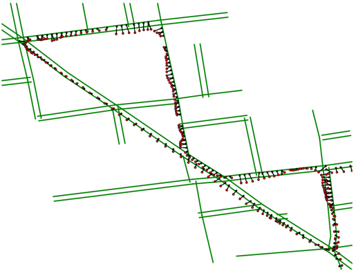
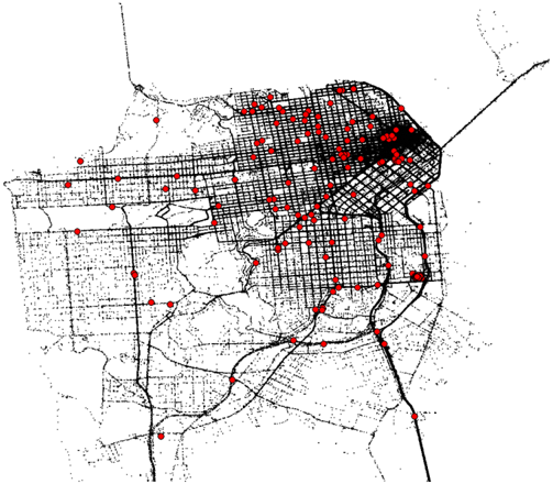
GPS receivers have enjoyed a widespread use in transportation and they are rapidly becoming a commodity. They offer unique capabilities for tracking fleets of vehicles (for companies), and routing and navigation (for individuals). These receivers are usually attached to a car or a truck, also called a probe vehicle , and they relay information to a base station using the data channels of cellphone networks (3G, 4G). A typical datum provided by a probe vehicle includes an identifier of the vehicle, a (noisy) position and a timestamp 1 . Figure 1 graphically presents a subset of probe data collected by Mobile Millennium . In addition to these geolocalization attributes, data points contain other attributes such as heading, speed, etc. We will show how this additional information can be integrated in the rest of the framework presented in this article.

The two most important characteristics of GPS data for traffic estimation purposes are the GPS localization accuracy and the sampling strategy followed by the probe vehicle. In order to reduce power consumption or transmission costs,

1 The experiments in this article use GPS observations only. However, nothing prevents the application of the algorithms presented in this article to other types of localized data.

probe vehicles do not continuously report their location to the base station. The probe data currently available are generated using a combination of the two following strategies:

• Geographical sampling : GPS probes are programmed to send information in the vicinity of virtual landmarks [23]. This concept was popularized by Nokia under the term Virtual Trip Line [19]. These landmarks are usually laid over some predetermined route followed by drivers.
• Temporal sampling : GPS probes send their position at fixed rate. The critical factor is then the temporal resolution of the probe data. A low temporal resolution carries some uncertainty as to which trajectory was followed. A high temporal resolution gives access to the complete and precise trajectory of the vehicle. However, the device usually consumes more power and communication bandwidth.

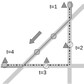
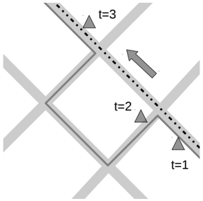
In the case of a high temporal resolution (typically, a frequency greater than an observation per second), some highly successful methods have been developed for continuous estimation [38], [24], [12]. However, most data collected at large scale today is generated by commercial fleet vehicles. It is primarily used for tracking the vehicles and usually has a low temporal resolution (1 to 2 minutes) [27], [21], [35], [9]. In the span of a minute, a vehicle in a city can cover several blocks. Therefore, information on the precise path followed by the vehicle is lost. Furthermore, due to GPS localization errors, recovering the location of a vehicle that just sent an observation is a non trivial task: there are usually several streets that could be compatible with any given GPS observation. Simple deterministic algorithms to reconstruct trajectories fail due to misprojection (Figure 3) or shortcuts (Figure 2). Such shortcomings have motivated our search for a principled approach that jointly considers the mapping of observations to the network and the reconstruction of the trajectory.

The problem of mapping data points onto a map can be traced back to 1980 [3]. Researchers started systematic studies after the introduction of the GPS system to civilian applications in the 1990s [31]. These early approaches followed a geometric perspective, associating each observation datum to some point in the network [40]. Later, this projection technique was refined to use more information such as heading and road curvature. This greedy matching, however, leads to poor trajectory reconstruction since it does not consider the path leading up to a point [42]. New deterministic algorithms emerged to directly match partial trajectories to the road by using the topology of the network [16] and topological metrics based on the Fréchet distance [8], [39]. These deterministic algorithms cannot readily cope with ambiguous observations [24], and were soon expanded into probabilistic frameworks. A number of implementations were explored: particle filters [29], [17], Kalman filters [28], Hidden Markov Models [4], and less mainstream approaches based on Fuzzy Logic and Belief Theory.

Two types of information are missing in a sequence of GPS readings: the exact location of the vehicle on the road network when the observation was emitted, and the path followed from the previous location to the new location. These problems are correlated. The aforementioned approaches focus on highfrequency sampling observations, for which the path followed is extremely short (less than a few hundred meters, with very few intersections). In this context, there is usually a dominant path that starts from a well-defined point, and Bayesian filters accurately reconstruct paths from observations [28], [38], [17]. When sampling rates are lower and observed points are further apart, however, a large number of paths are possible between two points. Researchers have recently focused on efficiently identifying these correct paths and have separated the joint problem of finding the paths and finding the projections into two distinct problems. The first problem is path identification and the second step is projection matching [43], [4], [42], [15], [37]. Some interesting trajectories mixing points and paths that use a voting scheme have also recently been proposed [42]. Our filter aims at solving the two problems at the same time, by considering a single unified notion of trajectory .

The path inference filter is a probabilistic framework that aims at recovering trajectories and road positions from lowfrequency probe data in real time, and in a computationally efficient manner. As will be shown, the performance of the filter degrades gracefully as the sampling frequency decreases, and it can be tuned to different scenarios (such as real time estimation with limited computing power or offline, high accuracy estimation).

The filter is justified from the Bayesian perspective of the noisy channel and falls into the general class of Conditional Random Fields [22]. Our framework can be decomposed into the following steps:

• Map matching : each GPS measurement from the input is projected onto a set of possible candidate states on the road network.
• Path discovery: admissible paths are computed between pairs of candidate points on the road network.
• Filtering : probabilities are assigned to the paths and the points using both a stochastic model for the vehicle dynamics and probabilistic driver preferences learned from data.

According to the very exhaustive review by Quddus et al. [30], most map-matching approaches fall into one of the four categories:

1. 'Geometric' methods, which pick the closest matching point. The distance metric itself is the subject of variations by different authors.
2. 'Weighted topological' methods, which use connectivity information between links and various ways to weight the different paths.
3. 'Probabilistic' methods, which combine variance information about the points and topological information about the paths in a simple way.
4. 'Advanced' methods, which encompass everything more complicated: Kalman Filtering, Particle Filtering, Belief Theory [13] and Fuzzy Logic [34]. 2

2 Note that 'probabilistic' models, as well as most of the 'advanced' models (Kalman Filtering, Particle Filtering, Hidden Markov Models) fall under the general umbrella of Dynamic Bayesian Filters , presented in great detail in [38]. As such, they deserve a common theoretical treatment, and in particular all suffer from the same pitfalls detailed in Section III.

The path inference filter presents a number of compelling advantages over the work found in the current literature:

1. The approach presents a general framework grounded in established statistical theory that encompasses, as special cases, most techniques presented as 'geometric', 'topological' or 'probabilistic'. In particular, it combines information about paths, points and network topology in a single unified notion of trajectory.
2. Nearly all work on Map Matching is segmented into (and presents results for) either high-frequency or lowfrequency sampling. The path inference filter performs as well as the current state-of-the-art approaches for sampling rates less than 30 seconds, and improves upon the state of the art [43], [42] by a factor of more than 10% for sampling intervals greater than 60 seconds 3 . We also analyze failure cases and we show that the output provided by the path inference filter is always 'close' to the true output for some metric.
3. As will be seen in Section III, most existing approaches (which are based on Dynamic Bayesian Networks) do not work well at lower frequencies due to the selection bias problem . Our work directly addresses this problem by performing inference on a Random Field.
4. The path inference filter can be used with complex path models such as those used in [4] and [15]. In the present article, we restrict ourselves to a class of models (the exponential family distributions) that is rich enough to provide insight on the driving patterns of the vehicles. Furthermore, when using this class of models, the learning of new parameters leads to a convex problem formulation that is fast to solve. These parameters can be learned using standard Machine Learning algorithms, even when no ground truth is available.
5. With careful engineering, it is possible to achieve high throughput on large-scale networks. Our reference implementation achieves an average throughput of hundreds of GPS observations per second on a single core in real time. Furthermore, the algorithm scales well on multiple cores and has achieved average throughput of several thousands of points per second on a multicore architecture.

Algorithms often need to trade off accuracy for timeliness, and are considered either 'local' (greedy) or 'global' (accumulating some number of points before returning an answer) [42]. The path inference filter is designed to work across the full spectrum of accuracy versus latency. As we will show, we can still achieve good accuracy by delaying computations by only one or two time steps.

II. PATH DISCOVERY

The road network is described as a directed graph N = ( V , E ) in which the nodes are the street intersections and the edges are the streets, referred to in the text as the links of the road network. Each link is endowed with a number of

3 Performance comparisons are complicated by the lack of a single agreedupon benchmark dataset. Nevertheless, the city we study is complex enough to compare favorably with cities studied with other works.

physical attributes (speed limit, number of lanes, type of road, etc.). Given a link of the road network, the links into which a vehicle can travel will be called outgoing links , and the links from which it can come will be called the incoming links. Every location on the road network is completely specified by a given link l and offset o on this link. The offset is a non-negative real number bounded by the length of the corresponding link, and represents the position on the link. At any time, the state x of a vehicle consists of its location on the road network and some other optional information such as speed, or heading. For our example we consider that the state is simply the location on one of the road links (which are directed). Additional information such as speed, heading, lane, etc. can easily be incorporated into the state:

Furthermore, for the remainder of this article we consider trajectory inference for a single probe vehicle.

A. From GPS points to discrete vehicle states

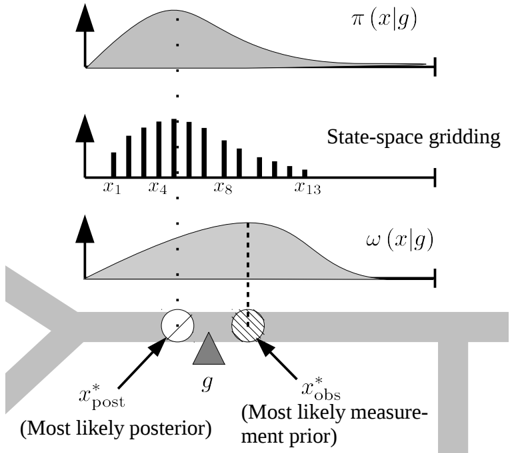
The points are mapped to the road following a Bayesian formulation. Consider a GPS observation g . We study the problem of mapping it to the road network according to our knowledge of how this observation was generated. This generation process is represented by a probability distribution ω ( g | x ) that, given a state x , returns a probability distribution over all possible GPS observations g . Such distributions ω will be described in Section III-D. Additionally, we may have some prior knowledge over the state of the vehicle. For example, some links may be visited more often than others, and some positions on links may be more frequent, such as when vehicles accumulate at the intersections. This knowledge can be encoded in a prior distribution Ω( x ) . Under this general setting, the state of a vehicle, given a GPS observation, can be computed using Bayes' rule:

The letter π will define general probabilities, and their dependency on variables will always be included. This probability distribution is defined up to a scaling factor in order to integrate to 1 . This posterior distribution is usually complicated, owing to the mixed nature of the state. The state space is the product of a discrete space over the links and a continuous space over the link offsets. Instead of representing it in closed form, some sampled values are considered: for each link l i , a finite number of states from this link are elected to represent the posterior distribution of the states on this link π ( o | g, l = l i ) . A first way of accomplishing this task is to grid the state space of each link, as illustrated in Figure 4. This strategy is robust against the observation errors described in Section II-B, but it introduces a large number of states to consider. Furthermore, when new GPS values are observed every minute, the vehicle can move quite extensively between updates. The grid step is usually small compared to the distance traveled. Instead of defining a coarse grid over each link, another approach is to use some most likely state on each link. Since our state is the pair of a link and an offset on this link, this corresponds to selecting the most likely offset on each state:

In practice, the probability distribution π ( x | g ) decays rapidly, and can be considered overwhelmingly small beyond a certain distance from the observation g . Links located beyond a certain radius need not be considered valid projection links, and may be discarded.

In the rest of this article, the boldface symbol x will denote a (finite) collection of states associated with a GPS observation g that we will use to represent the posterior distribution π ( x | g ) , and the integer I will denote its cardinality: x = ( x i ) 1: I . These points are called candidate state projections for the GPS measurement g . These discrete points will then be linked together through trajectory information that takes into account

the trajectory and the dynamics of the vehicle. We now mention a few important points for a practical implementation.

The prior distribution. A Bayesian formulation requires that we endow the state x with a prior distribution Ω( x ) that expresses our knowledge about the distribution of points on a link. When no such information is available, since the offset is continuous and bounded on a segment, a natural non-informative prior is the uniform distribution over offsets: Ω ∼ U ([0 , length ( l )]) . In this case, maximizing the posterior is equivalent to maximizing the conditional distribution from the generative model:

Having mapped GPS points into discrete points on the road network, we now turn our attention to connecting these points by paths in order to form trajectories.

B. From discrete vehicle states to trajectories

At each time step t , a GPS point g t (originating from a single vehicle) is observed. This GPS point is then mapped onto I t different candidate states denoted x t = x t 1 · · · x t I t . Because this set of projections is finite, there is only a (small) finite number J t of paths that a vehicle can have taken while

moving from some state x t i ∈ x t to some state x t +1 i ′ ∈ x t +1 . We denote the set of candidate paths between the observation g t and the next observation g t +1 by p t :

Each path p t j goes from one of the projection states x t i of g t to a projection state x t +1 i ′ of g t +1 . There may be multiple pairs of states to consider, and between each pair of states, there are typically several paths available (see Figure 5). Lastly, a trajectory is defined by the succession of states and paths, starting and ending with a state:

where x 1 is one element of x 1 , p 1 of p 1 , and so on.

Due to speed limits leading to lower bounds on achievable travel times on the network, there is only a finite number of paths a vehicle can take during a time interval ∆ t . Such paths can be computed using standard graph search algorithms. The depth of the search is bounded by the maximum distance a vehicle can travel on the network at a speed v max within the time interval between each observation. An algorithm that

performs well in practice is the A* algorithm [18], a common graph search algorithm that makes use of a heuristic to guide its search. The cost metric we use here is the expected travel time on each link, and the heuristic is the shortest geographical distance, properly scaled so that it is an admissible heuristic.

The case of backward paths. It is convenient and realistic to assume that a vehicle always drives forward , i.e. in the same direction of a link 4 . In our notation, a vehicle enters a link at offset 0 , drives along the link following a non-decreasing offset, and exits the link when the offset value reaches the total length of the link. However, due to GPS noise, the most likely state projection of a vehicle waiting at a red light may appear to go backward, as shown in Figure 6. This leads to incorrect transitions if we assume that paths only go forward on a link. Three approaches to solve this issue are discussed, depending on the application:

1. It is possible to keep a single state for each link (the most likely) and explore some backward paths. These paths are assumed to go backward because of observation noise. This solution provides connected states at the expense of physical consistency : all the measurements are correctly mapped to their most likely location, but the trajectories themselves are not physically acceptable. This is useful for applications that do not require connectedness between pairs of states, for example when computing a distribution of the density of probe data per link.
2. It is also possible to disallow backward paths and consider multiple states per link, such as a grid over the state space. A vehicle never goes backward, and in this case the filter can generally account for the vehicle not moving by associating the same state to successive observations. All the trajectories are physically consistent and the posterior state density is the same as the probability density of the most likely states, but is

4 Reverse driving is in some cases even illegal. For example, the laws of Glendale, Arizona, prohibit reverse driving.

more burdensome from a computational perspective (the number of paths to consider grows quadratically with the number of states).

1. Finally it is possible to disallow backward paths and use a sparse number of states. The path connectivity issue is solved using some heuristics. Our implementation creates a new state projection on a link l using the following approach:

Given a new observation g , and its most likely state projection x ∗ = ( l, o ∗ ) :

1. If no projection for the link l was found at the previous time step, return x ∗
2. If such a projection x before = ( l, o before ) existed, return x = ( l, max( o before , o ∗ ))

With this heuristic, all the points will be well connected, but the density of the states will not be the same as the density of the most likely reconstructed states.

In summary, the first solution is better for density estimations and the third approach works better for travel time estimations. The second option is currently only used for high-frequency offline filtering, for which paths are short, and for which more expensive computations is an acceptable cost.

Handling errors Maps may contains some inaccuracies, and may not cover all the possible driving patterns. Two errors were found to have a serious effect on the performance of the filter:

• Out of network driving: This usually occurs in parking lots or commercials driveways.
• Topological errors: Some links may be missing on the base map, or one-way streets may have changed to twoway streets. These situations are handled by running flow analysis on the trajectory graph . For every new incoming GPS point, after computing the paths and states, it is checked if any candidate position of the first point of the trajectory is reachable from any reachable candidate position on the latest incoming point, or equivalently if the trajectory graph has a positive flow. The set of state projections of an observation may end up being disconnected from the start point even if at every step, there exists a set of paths between each points. In this situation, the probability model will return a probability of 0 (non-physical trajectories) for any trajectory. If a point becomes unreachable from the start point, the trajectory is broken, and restarted again from this point. Trajectory breaks were few (less than a dozen for our dataset), and a visual inspection showed that the vehicle was not following the topology of the network and instead made U-turns or breached through one-way streets.

III. DISCRETE FILTERING USING A CONDITIONAL RANDOM FIELD

In the previous section, we reduced the trajectory reconstruction problem to a discrete selection problem between sets of candidate projection points, interleaved with sets of candidate paths. A probabilistic framework can now be applied to infer a reconstructed trajectory τ or probability distributions over candidate candidate states and candidate paths. Without further assumptions, one would have to enumerate and compute probabilities for every possible trajectory. This is not possible for long sequences of observations, as the number of possible trajectories grows exponentially with the number of observations chained together. By assuming additional independence relations, we turn this intractable inference problem into a tractable one.

A. Conditional Random Fields to weight trajectories

The observation model provides the joint distribution of a state on the road network given an observation. We have described the noisy generative model for the observations in Section II-A. Assuming that the vehicle is at a point x , a GPS observation g will be observed according to a model ω that describes a noisy observation channel. The value of g only depends on the state of the vehicle, i.e. the model reads ω ( g | x ) . For every time step t , assuming that the vehicle is at the location x t , a GPS observation g t is created according to the distribution ω ( g t | x t ) .

Additionally, we endow the set of all possible paths on the road network with a probability distribution. The transition model η describes the preference of a driver for a particular path. In probabilistic terms, it provides a distribution η ( p ) defined over all possible paths p across the road network. This distribution is not a distribution over actually observed paths as much as a model of the preferences of the driver when given the choice between several options.

We introduce the following Markov assumptions .

• Given a start state x start and an end state x end, the path p followed by the vehicle between these two points will only depend on the start state, the end state and the path itself. In particular, it will not depend on previous paths or future paths.
• Consider a state x followed by a path p next and preceded by a path p previous, and associated to a GPS measurement g . Then the paths taken by the vehicle are independent from the GPS measurement g if the state x is known. In other words, the GPS measurement does not add subsequent information given the knowledge of the state of the vehicle.

Since a state is composed of an offset and a link, a path is completely determined by a start state, an end state and a list of links in between. Conditional on the start state and end state, the number of paths between these points is finite (it is the number of link paths that join the start link and the end link).

Not every path is compatible with given start point and end point: the path must start at the start state and must end at the end state. We formally express the compatibility between a state x and the start state of a path p with the compatibility function δ :

Similarly, we introduce the compatibility function ¯ δ to express the agreement between a state and the end state of

)

)

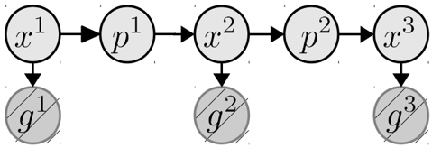
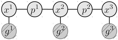
Figure 7. Illustration of the Conditional Random Field defined over a trajectory τ = x 1 p 1 x 2 p 2 x 3 and a sequence of observations g 1:3 . The gray nodes indicate the observed values. The solid lines indicate the factors between the variables: ω ( g t | x t ) between a state x t and an observation g t , δ ( x t , p t ) η ( p t ) between a state x t and a path p t and ¯ δ ( p t , x t +1 ) between a path p t and a subsequent state x t +1 .

a path:

Given a sequence of observations g 1: T = g 1 · · · g T and an associated trajectory τ = x 1 p 1 · · · x T , we define the unnormalized score, or potential , of the trajectory as:

The non-negative function φ is called the potential function. A trajectory τ is said to be a compatible trajectory with the observation sequence g 1: T if φ ( τ | g 1: T ) > 0 . When properly scaled, the potential φ defines a probability distribution over all possible trajectories, given a sequence of observations:

The variable Z , called the partition function , is the sum of the potentials over all the compatible trajectories:

We have combined the observation model ω and the transition model η into a single potential function φ , which defines an unnormalized distribution over all trajectories. Such a probabilistic framework is called a Conditional Random Field (CRF) [22]. A CRF is an undirected graphical model which is defined as the unnormalized product of factors over cliques of factors (see Figure 7). There can be an exponentially large number of paths, so the partition function cannot be computed by simply summing the value of φ over every possible trajectory. As will be seen in Section IV, the value of Z needs to be computed only during the training phase. Furthermore it can be computed efficiently using dynamic programming.

The case against the Hidden Markov Model approach . The classical approach to filtering in the context of trajectories is based on Hidden Markov Models (HMMs), or their generalization, Dynamic Bayesian Networks (DBNs) [26]: a sequence of states and trajectories form a trajectory, and the coupling of

)

)

Figure 8. A Dynamic Bayesian Network (DBN) commonly used to model the trajectory reconstruction problem. The arrows indicated the directed dependencies of the variables. The GPS observations g t are generated from states x t . The unobserved paths p t are generated from a state x t , following a transition probability distribution ˆ π ( p | x ) . The transition from a path p t to a state x t follows the transition model ˆ π ( x | p ) .

trajectories and states is done using transition models ˆ π ( x | p ) and ˆ π ( p | x ) . See Figure 8 for a representation.

This results in a chain-structured directed probabilistic graphical model in which the path variables p t are unobserved. Depending on the specifics of the transition models, ˆ π ( x | p ) and ˆ π ( p | x ) , probabilistic inference has been done with Kalman filters [28], [29], the forward algorithm or the Viterbi algorithm [4], [5], or particle filters [17].

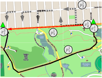
Hidden Markov Model representations, however, suffer from the selection bias problem , first noted in the labeling of words sequences [22], which makes them not the best fit for solving path inference problems. Consider the example trajectory τ = x 1 p 1 x 2 observed in our data, represented in Figure 9. For clarity, we consider only two states x 1 1 and x 1 2 associated with the GPS reading g 1 and a single state x 2 1 associated with g 2 . The paths ( p 1 j ) j between x 1 and x 2 may either be the lone path p 1 1 from x 1 1 to x 2 1 that allows a vehicle to cross the Golden Gate Park, or one of the many paths between Cabrillo Street and Fulton Street that go from x 1 2 to x 1 , including p 1 3 and p 1 2 . In the HMM representation, the transition probabilities must sum to 1 when conditioned on a starting point. Since there is a single path from x 1 2 to x 2 , the probability of taking this path from the state x 1 1 will be ˆ π ( p 1 1 | x 1 1 ) = 1 so the overall probability of this path is ˆ π ( p 1 1 | g 1 ) = ˆ π ( x 1 1 | g 1 ) . Consider now the paths from x 1 2 to x 2 1 : a lot of these paths will have a similar weight, since they correspond to different turns and across the lattice of streets. For each path p amongst these N paths of similar weight, Bayes' assumption implies ˆ π ( p | x 1 2 ) ≈ 1 N so the overall probability of this path is ˆ π ( p | g 1 ) ≈ 1 N ˆ π ( x 1 2 | g 1 ) . In this case, N can be large enough that ˆ π ( p 1 1 | g 1 ) ≥ ˆ π ( p | g 1 ) , and the remote path will be selected as the most likely path.

Due to their structures, all HMM models will be biased towards states that have the least expansions. In the case of a road network, this can be pathological. In particular, the HMM assumption will carry the effect of the selection bias as long as there are long disconnected segments of road. This can be particularly troublesome in the case of road networks since HMM models will end up being forced to assign too much weight to a highway (which is highly disconnected) and not enough to the road network alongside the highway. Our model, which is based on Conditional Random Fields, does not have

this problem since the renormalization happens just once and is over all paths from start to end, rather than renormalizing for every single state transition independently.

Efficient filtering algorithms. Using the probabilistic framework of the CRF, we wish to infer:

• the most likely trajectory τ :

• the posterior distributions over the elements of the trajectory, i.e. the conditional marginals π ( x t | g 1: T ) and π ( p t | g 1: T )

As will be seen, both elements can be computed without having to obtain the partition function Z . The solution to both problems is a particular case of the Junction Tree algorithm [26] and can be computed in time complexity linear in the time horizon by using a dynamic programing formulation. Computing the most likely trajectory is a particular instantiation of a standard dynamic programing algorithm called the Viterbi algorithm [14]. Using a classic Machine Learning algorithm for chain-structured junction trees (the forwardbackward algorithm [33], [6]), all the conditional marginals can be computed in two passes over the variables. In the next section, we detail the justification for the Viterbi algorithm and in Section III-C we describe an efficient implementation of the forward-backward algorithm in the context of this application.

B. Finding the most likely path

For the rest of this section, we fix a sequence of observations g 1: T . For each observation g t , we consider a set of candidate state projections x t . At each time step t ∈ [1 · · · T -1] , we consider a set of paths p t , so that each path p t from p t starts from some state x t ∈ x t and ends at some state x t +1 ∈ x t +1 . We will consider the set ς of valid trajectories in the Cartesian space defined by these projections and these paths:

In particular, if I t is the number of candidate states associated with g t (i.e. the cardinal of x t ) and J t is the number of candidate paths in p t , then there are at most ∏ T 1 I t ∏ T -1 1 J t possible trajectories to consider. We will see, however, that most likely trajectory τ ∗ can be computed in O ( TI ∗ J ∗ ) computations, with I ∗ = max t I t and J ∗ = max t J t .

The partition function Z does not depend on the current trajectory τ and need not be computed when solving Equation 1:

Call φ ∗ ( g 1: T ) the maximum value over all the potentials of the trajectories compatible with the observations g 1: T :

The trajectory τ that realizes this maximum value is found by tracing back the computations. For example, some pointers to the intermediate partial trajectories can be stored to trace back the complete trajectory, as done in the referring implementation [1]. This is why we will only consider the computation of this maximum. The function φ depends on the probability distributions ω and η , left undefined so far. These distributions will be presented in depth in Sections III-D and III-E.

It is useful to introduce notation related to a partial trajectory . Call τ 1: t the partial trajectory until time step t :

For a partial trajectory, we define some partial potentials φ ( τ 1: t | g 1: t ) that depend only on the observations seen so far:

For each time step t , given a state index i ∈ [1 , I t ] we introduce the potential function for trajectories that end at the state x t i :

One sees:

The partial potentials defined in Equation (2) follow an inductive identity:

By using this identity, the maximum potential φ ∗ can be computed efficiently from the partial maximum potentials φ t i . The computation of the trajectory that realizes this maximum potential ensues by tracing back the computation to find which partial trajectory realized φ t i for each step t .

C. Trajectory filtering and smoothing

We now turn our attention to the problem of computing the marginals of the posterior distributions over the trajectories, i.e. the probability distributions π ( x t | g 1: T ) and π ( p t | g 1: T ) for all t . We introduce some additional notation to simplify the subsequent derivations. The posterior probability ¯ q t i of the vehicle being at the state x t i ∈ x t at time t , given all the observations g 1: T of the trajectory, is defined as:

The operator ∝ indicates that this distribution is defined up to some scaling factor, which does not depend on x or p (but may depend on g 1: T ). Indeed, we are interested in the probabilistic weight of a state x t i relative to the other possible states x t i ′ at the state time t (and not to the actual, unscaled value of π ( x t i | g 1: T ) ). This is why we consider (¯ q t i ) i as a choice between a (finite) set of discrete variables, one choice per possible state x t i . A natural choice is to scale the distribution ¯ q t i so that the probabilistic weight of all possibilities is equal to 1:

From a practical perspective, ¯ q t can be computed without the knowledge of the partition function Z . Indeed, the only required elements are the unscaled values of π ( x t i | g 1: T ) for each i . The distribution ¯ q t = (¯ q t i ) i is a multinomial distribution between I t choices, one for each state. The quantity ¯ q t i has a clear meaning: it is the probability that the vehicle is in state x t i , when choosing amongst the set ( x t i ′ ) 1 ≤ i ≤ I t , given all the observations g 1: T .

For each time t and each path index j ∈ [1 · · · J t ] , we also introduce (up to a scaling constant) the discrete distribution over the paths at time t given the observations g 1: T :

which are scaled so that ∑ 1 ≤ j ≤ J t r t j = 1 .

This problem of smoothing in CRFs is a classic application of the Junction Tree algorithm to chain-structured graphs [26]. For the sake of completeness, we derive an efficient smoothing algorithm using our notations.

The definition of π ( x t i | g 1: T ) requires summing the potentials of all the trajectories that pass through the state x t i at time t . The key insight for efficient filtering or smoothing is to make use of the chain structure of the graph, which lets us factorize the summation into two terms, each of which can be computed much faster than the exponentially large summation. Indeed, one can show from the structure of the clique graph that the following holds for all time steps t :

The first term of the pair corresponds to the effect that the past and present observations ( g 1: t ) have on our belief of the present state x t . The second term corresponds to the effect that the future observations ( g t +1: T ) have on our estimation of the present state. The terms π ( x t | g 1: t ) are related to each other by an equation that propagates forward in time, while the terms π ( x t | g t +1: T ) are related through an equation that goes backward in time. This is why we call π ( x t | g 1: t ) the forward distribution for the states , and we denote it 5 by ( - → q t i ) 1 ≤ i ≤ I t :

The distribution - → q t i is proportional to the posterior probability π ( x t i | g 1: t ) and the vector - → q t = ( - → q t i ) i is normalized so that ∑ I t i =1 - → q t i = 1 . We do this for the paths, by defining the forward distribution for the paths :

Again, the distributions are defined up to a normalization factor so that each component sums to 1 .

In the same fashion, we introduce the backward distributions for the states and the paths:

Using this set of notations, Equation (4) can be rewritten:

Furthermore, - → r t and - → q t are related through a pair of recursive equations:

5 The arrow notation indicates that the computations for - → q t i will be done forward in time.

Similarly, the backward distributions can be defined recursively, starting from t = T :

Details of the forward algorithm and backward algorithm are provided in the Algorithm 1 and Algorithm 2 below. The complete algorithm for smoothing is detailed in the Algorithm 3 below.

Algorithm 1 Description of forward recursion

Given a sequence of observations g 1: T , a sequence of sets of candidate projections x 1: T and a sequence of sets of candidate paths p 1: T -1 :

Initialize the forward state distribution:

For every time step t from 1 to T -1 :

Compute the forward probability over the paths:

Normalize r

Compute the forward probability over the states:

∀

i

= 1

· · ·

I

t

+1

:

Return the set of vectors ( - → q t ) t and ( - → r t ) t

Normalize q

The above smoothing algorithm requires all the observations of a trajectory in order to run. We have presented so far an a posteriori algorithm that requires full knowledge of measurements g 1: T . In this form, it is not directly suitable for real-time applications that involve streaming data, for which the data is available up to t only. However, this algorithm can be adapted for a variety of scenarios:

• Smoothing , also called offline filtering . This corresponds to getting the best estimate given all observations, i.e. to computing π ( x t | g 1: T ) . The Algorithm 3 describes this procedure.
• Tracking, filtering , or online estimation. This usage corresponds to updating the current state of the vehicle as soon as a new streaming observation is available, i.e. to computing π ( x t | g 1: t ) . This is exactly the case the forward algorithm (Algorithm 1) is set to solve. If one is

Algorithm 2 Description of backward recursion

Given a sequence of observations g 1: T , a sequence of sets of candidate projections x 1: T and a sequence of sets of candidate paths p 1: T -1 :

Initialize the backward state distribution

For every time step t from T -1 to 1:

Compute the forward probability over the paths:

Compute the forward probability over the states:

Return the set of vectors ( ← -q t ) t and ( ← -r t ) t

Algorithm 3 Trajectory smoothing algorithm

Given a sequence of observations g 1: T , a sequence of sets of candidate projections x 1: T and a sequence of sets of candidate paths p 1: T -1 :

Compute

q

and t For every time step t :

Normalize r t

t

Normalize q t

Return the set of vectors ( q t ) t and ( r t ) t simply interested in the most recent estimate, then only the previous forward distribution - → q t needs to be kept, and all distributions - → q t -1 · · · - → q 1 at previous times can be discarded. This application minimizes the latency and the computations at the expense of the accuracy.

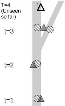
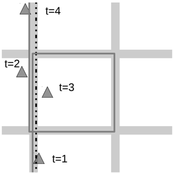
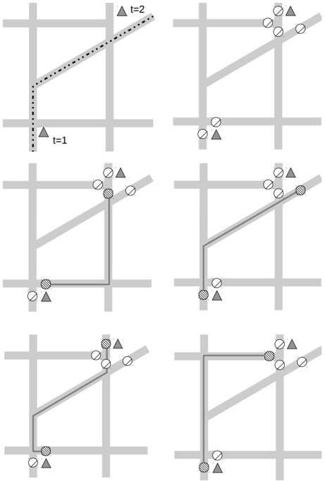
• Lagged smoothing , or lagged filtering . A few points of data are stored and processed before returning a result. Algorithm 4 details this procedure, which involves computing π ( x t | g 1: t + k ) for some k > 0 . A trade-off is being made between the latency and the accuracy, as the information from the points g t +1: t + k is used to update the estimate of the state x t . As shown in Section VI, even for small values of k , such a procedure can bring significant improvements in the accuracy while keeping the latency within reasonable bounds. A common ambiguity solved by lagged smoothing is presented in Figure 10.

D. Observation model

We now describe the observation model ω . The observation probability is assumed only to depend on the distance between the point and the GPS coordinates. We take an isoradial

r

using the backward algorithm.

Algorithm 4 Lagged smoothing algorithm

Given an integer k > 0 , and a LIFO queue of observations: Initialize the queue to the empty queue.

When receiving a new observation g t :

Push the observation in the queue

Run the forward filter on this observation

If t > k :

Run the backward filter on the queue Compute q t -k , r t -k on the first element of the queue Pop the queue and return q t -k and r t -k

Gaussian noise model:

in which the function d is the distance function between geocoordinates. The standard deviation σ is assumed to be constant over all the network. This is not true in practice because of well documented urban canyoning effects [10], [36], [37] and satellite occlusions. Updating the model accordingly presents no fundamental difficulty, and can be done by geographical clustering of the regions of interest. Using the estimation techniques described later in Section IV-C and Section IV-D, an estimate of σ between 10 and 15 meters could be estimated for data of interest in this article.

E. Driver model

The second model to consider is the driver behavior model. This model assigns a weight to any acceptable path on the road network. We consider a model in the exponential family , in which the weight distribution over any path p only depends on a selected number of features ϕ ( p ) ∈ R K of the path. Possible features include the length of the path, the number of stop signs, and the speed limits on the road. The distribution is parametrized by a vector µ ∈ R K so that the logarithm of the distribution of paths is a linear combination of the features of the path:

The function ϕ is called the feature function, and the vector µ is called the behavioral parameter vector , and simply encodes a weighted combination of the features.

In a simple model the vector ϕ ( p ) may be reduced to a single scalar, such as the length of the path. Then the inverse of µ , a length, can be interpreted as a characteristic length. This model simply states that the driver has a preference for shorter paths, and µ -1 indicates how aggressively this driver wants to follow the shortest path. Such a model is explored in Section (VI). Other models considered include the mean speed and travel times, the stop signs and signals, and the turns to the right or to the left.

In the Mobile Millennium system, the path inference filter is the input to a model designed to learn travel times, so the feature function does not include dynamic features such as the current travel time. Assuming this information is available, it would be easy to add as a feature.

IV. TRAINING PROCEDURE

The procedure detailed so far requires the calibration of the observation model and the path selection model by setting some values for the weight vector µ and the standard deviation σ . Using standard machine learning techniques, we maximize the likelihood of the observations with respect to the parameters, and we evaluate the result against heldout trajectories using several metrics detailed in Section VI. Computing likelihood will require the computation of the partition function (which depends on µ and σ ). We first present a procedure that is valid for any path or point distributions that belong to the exponential family , and then show how the models we presented in Section III fit into this framework.

A. Learning within the exponential family and sparse trajectories

There is a striking similarity between the state variables x 1: T and the path variables p 1: T especially between the forward and backward distributions introduced in Equation (5). This suggests to generalize our procedure to a context larger than states interleaved with paths. Indeed, each step of choosing a path or a variable corresponds to making a choice between a finite number of possibilities, and there is a limited number of pairwise compatible choices (as encoded by the functions δ and ¯ δ ). Following a trajectory corresponds to choosing a new state (subject to the compatibility constraints of the previous state). In this section, we introduce the proper notation to generalize our learning problem, and then show how this learning problem can be efficiently solved. In the next section, we will describe the relation between the new variables we are going to introduce and the parameters of our model.

Consider a joint sequence of multinomial random variables z 1: L = z 1 · · · z L drawn from some space ∏ L l =1 { 1 · · · K l } where K l is the dimensionality of the multinomial variable z l . Given a realization z 1: L from z 1: L , we define a nonnegative potential function ψ ( z 1: L ) over the sequence of variables. This potential function is controlled by a parameter vector θ ∈ R M : ψ ( z 1: L ) = ψ ( z 1: L ; θ ) 6 . Furthermore, we assume that this potential function is also defined and nonnegative over any subsequence ψ ( z 1: l ) . Lastly, we assume that there exists at least one sequence z 1: L that has a positive potential. As in the previous section, the potential function ψ , when properly normalized, defines a probability distribution of density π over the variables z , and this distribution is parametrized by the vector θ :

with Z = ∑ z ψ ( z ; θ ) called the partition function . We will show the partition function defined here is the partition function introduced in Section III-C.

6 The semicolon notation indicates that this function is parametrized by θ , but that θ is not a random variable.

We assume that ψ is an unscaled member of the exponential family : it is of the form:

In this representation, h is a non-negative function of z which does not depend on the parameters, the operator · is the vector dot product, and the vectors T l ( z l ) are vector mappings from the realization z l to R M for some M ∈ N , called feature vectors . Since the variable z l is discrete and takes on values in { 1 · · · K l } , it is convenient to have a specific notation for the feature vector associated with each value of this variable:

The sequence of variables z represents the choices associated with a single trajectory, i.e. the concatenation of the x s and p s. In general, we will observe and would like to learn from multiple trajectories at the same time. This is why we need to consider a collection of variables ( z ( u ) ) u , each of which follows the form above and each of which we can define a potential ψ ( z ( u ) ; θ ) and a partition function Z ( u ) ( θ ) for. There the variable u indexes the set of sequences of observations, i.e. the set of consecutive GPS measurements of a vehicle. Since each of these trajectories will take place on a different portion of the road network, each of the sequences z ( u ) will have a different state space. For each of these sequences of variables z ( u ) , we observe the respective realizations z ( u ) (which correspond to the observation of a trajectory), and we wish to infer the parameter vector θ ∗ that maximizes the likelihood of all the realizations of the trajectories:

where again the indexing u is for sets of measurements of a given trajectory. Similarly, the length of a trajectory is indexed by u : L ( u ) . From Equation 11, it is clear that the log-likelihood function simply sums together the respective likelihood functions of each trajectory. For clarity, we consider a single sequence z ( u ) only and we remove the indexing with respect to u . With this simplification, we have for a single trajectory:

The first part of Equation (12) is linear with respect to θ and log Z ( θ ) is concave in θ (it is the logarithm of a sum of exponentiated linear combinations of θ [7]) . As such, maximizing Equation (12) yields a unique solution (assuming no singular parametrization), and some superlinear algorithms exist to solve this equation [7]. These algorithms rely on the computation of the gradient and the Hessian matrix of log Z ( θ ) . We now detail some closed-form recursive formulas to compute these elements.

1) Efficient estimation of the partition function: A naive approach to the computation of the partition function Z ( θ ) leads to consider exponentially many paths. Most of these computations can be factored using dynamic programming 7 . Recall the definition of the partition function:

So far, the function h was defined in in a generic way (it is nonnegative and does not depend on θ ). We consider a particular shape that generalizes the functions δ and ¯ δ introduced in the previous section. In particular, the function h is assumed to be a binary function, from the Cartesian space ∏ L l =1 { 1 · · · K l } to { 0 , 1 } , that decomposes to the product of binary functions over consecutive pairs of variables:

in which every function h l is a binary indicator h l : { 1 · · · K l } × { 1 · · · K l -1 } → { 0 , 1 } . These functions h l generalize the functions δ and δ for arguments z equal to either the x s or the p s. It indicates the compatibility of the values of the instantiations z l and z l -1

Finally, we introduce the following notation. For each index l ∈ [1 · · · L ] and subindex i ∈ [1 · · · K l ] , we call Z l i the partial summation of all partial paths z 1: l that terminate at the value z l = i :

This partial summation can also be defined recursively:

The start of the recursion is for all i ∈ { 1 · · · K 1 } :

and the complete partition function is the summation of the auxiliary values:

Computing the partition function can be done in polynomial time complexity by a simple application of dynamic programming. By using sparse data structures to implement h , some additional savings in computations can be made 8 .

7 This is - again - a specific application of the junction tree algorithm. See [26] for an explanation of the general framework.

8 In particular, care should be taken to implement all the relevant computations in log-domain due to the limited precision of floating point arithmetic on computers. The reference implementation [1] shows one way to do it.

2) Estimation of the gradient: The estimation of the gradient for the first part of the log likelihood function is straightforward. The gradient of the partition function can also be computed using Equation (13):

The Hessian matrix can be evaluated in similar fashion:

B. Exponential family models

We now express our formulation of Conditional Random Fields to a form compatible with Equation (10).

Consider glyph[epsilon1] = σ -2 and θ the stacked vector of the desired parameters:

There is a direct correspondence between the path and state variables with the z variables introduced above. Let us pose L = 2 T -1 , then for all l ∈ [1 , L ] we have:

and the feature vectors are simply the alternating values of ϕ and d, completed by some zero values:

These formulas establish how we can transform our learning problem that involves paths and states into a more abstract problem that considers a single set of variables.

C. Supervised learning with known trajectories

The most straightforward way to learn µ and σ , or equivalently to learn the joint vector θ , is to maximize the likelihood of some GPS observations g 1: T , knowing the complete trajectory followed by the vehicle. For all time t , we also know which path p t observed was taken and which state x t observed produced the GPS observation g t . We make the assumption that the observed path p t observed is one of the possible path amongst the set of candidate paths ( p t j ) j :

and similarly, that the observed state x t observed is one of the possible states:

In this case, the values of r t and q t are known (they are the matching indexes), and the optimization problem of Equation (11) can be solved using methods outlined in Section IV-A.

D. Unsupervised learning with incomplete observations: Expectation-Maximization

Usually, only the GPS observations g 1: T are available; the values of r 1: T -1 and q 1: T (and thus z 1: L ) are hidden to us. In this case, we estimate the expected likelihood L , which is the expected value of the likelihood under the distribution over the assignment variables z 1: L :

The intuition behind this expression is quite natural: since we do not know the value of the assignment variable z , we consider the expectation of the likelihood over this variable. This expectation is done with respect to the distribution π ( z ; θ ) . The challenge lies in the dependency in θ of the very distribution used to take the expectation. Computing the expected likelihood becomes much more complicated than simply solving the optimization problem of (11).

One strategy is to find some 'fill in' values for z that would correspond to our guesses of which path was taken, and which point made the observation. However, such a guess would likely involve our model for the data, which we are currently trying to learn. A solution to this chicken and egg problem is the Expectation Maximization (EM) algorithm [25]. This algorithm performs an iterative projection ascent by assigning some distributions (rather than singular values) to every z l , and uses these distributions to updates the parameters µ and σ using the procedures seen in Section IV-C. This iterative procedure performs two steps:

1. Fixing some value for θ , it computes a distribution ˜ π ( z ) = π ( z ; θ )
2. It then uses this distribution ˜ π ( z ) to compute some new value of θ by solving the approximate problem in which the expectation is fixed with respect to θ :

This problem is significantly simpler than the optimization problem in Equation (14) since the expectation itself does not depend on θ and thus is not part of the optimization problem.

Under this procedure, the expected likelihood is shown to converge to a local maximum [26]. It can be shown that good values for the plug-in distribution ˜ π are simply the values of the posterior distributions π ( p t | g 1: T ) and π ( x t | g 1: T ) , i.e. the values q t and ¯ r t . Furthermore, owing to the particular shape

Algorithm 5 Expectation maximization algorithm for learning parameters without complete observations.

Given a set of sequences of observations, an initial value of θ Repeat until convergence:

For each sequence, compute r t and q t using Algorithm 3. For each sequence, update expected values of T t using (17) and (18).

Compute a solution of Problem (11) using these new values of T t .

of the distribution π ( z ) , taking the expectation is a simple task: we simply replace the value of the feature vector by its expected value under the distribution ˜ π ( z ) . More practically, we simply have to consider:

in which and

so that

These values of feature vectors plug directly into the supervised learning problem in Equation (11) and produce updated parameters µ and σ , which are then used in turn for updating the values of ¯ q and ¯ r and so on.

V. RESULTS FROM FIELD OPERATIONAL TEST

The path inference filter and its learning procedures were tested using field data through the Mobile Millennium system. Ten San Francisco taxicabs were fit with high frequency GPS (1 second sampling rate) in October 2010 during a twoday experiment. Together, they collected about seven hundred thousand measurement points that provided a high-accuracy ground truth. Additionally, the unsupervised learning filtering was tested on a significantly larger dataset: one day one-minute samples of 600 taxis from the same fleet, which represents 600 000 points. For technical reasons, the two datasets could not be collected the same day, but were collected the same day of the week (a Wednesday) three weeks prior to the highfrequency collection campaign. Even if the GPS equipment was different, both datasets presented the same distribution of GPS dispersion. Thus we evaluate two datasets collected from the same source with the same spatial features: a smaller set at high frequency, called 'Dataset 1', and a larger dataset sampled at 1 minute for which we do not know ground truth, called 'Dataset 2'.

Algorithm 6 Evaluation procedure

Given a set of high-frequency sequences of raw GPS data:

1. Map the raw high-frequency sequences on the road network
2. Run the Viterbi algorithm with default settings
3. Extract the most likely HF trajectory on the road network for each sequence
4. Given a set of projected HF trajectories:
5. Decimate the trajectories to a given sampling rate
6. Separate the set into a training subset and a test subset
7. Compute the best model parameters for a number of learning methods (most likely, EM with a simple model or a more complex model)
8. Evaluate the model parameters with respect to different computing strategies (Viterbi, online, offline, lagged smoothing) on the test subset

A. Experiment design

The testing procedure is described in Algorithm 6: the filter was first run in trajectory reconstruction mode (Viterbi algorithm) with settings and-tuned for a high-frequency application, using all the samples, in order to build a set of ground truth trajectories. The trajectories were then downsampled to different temporal resolutions and were used to test the filter in different configurations. The following features were tested:

• The sampling rate. The following values were tested: 1 second, 10 seconds, 30 seconds, one minute, one and a half minute and two minutes
• The computing strategy: pure filtering ('online' or forward filtering), fixed-lagged smoothing with a oneor two-point buffer ('1-lag' and '2-lag' strategies), Viterbi and smoothing ('offline', or forward-backward proce-

dure).

• Different models:
• -'Hard closest point': A greedy deterministic model that computes the closest point and then finds the shortest path to reach this closest point from the previous point. This non-probabilistic model is the baseline against which we make comparison on [16]. This greedy model may lead to non-feasible trajectories, for example by assigning an observation to a dead end link from which it cannot recover.
• -'Closest point' : A non-greedy version of 'Hard closest point'. Among all the feasible trajectories, this (naive, deterministic) model projects all the GPS data to their closest projections and then selects the shortest path between each projection. The computing strategy chosen is important because the filter may determine that some projections lead to dead end and force the trajectory to break.
• -'Shortest path': A naive model that selects the shortest path. Given paths of the same length, it will take the path leading to the closest point. The points projections are then recovered from the paths. This is similar to [15], [40].
• -'Simple' A simple model that considers two features that could be tuned by hand:
• ξ 1 : The length of the path
• ξ 2 : The distance of a point projection to its GPS coordinate

This model was trained on learning data by two procedures:

• ∗ Supervised learning, in which the true trajectory is provided to the learning algorithm leading to the 'MaxLL-Simple' model
• ∗ Unsupervised learning, which produced the model called 'EM-Simple'
• -'Complex' : A more complex model with a more diverse set of features, which is complicated enough to discourage manual tuning:
• The length of the path
• The number of stop signs along the path
• The number of signals (red lights)
• The number of left turns made by the vehicle at road intersections
• The number of right turns made by the vehicle at road intersections
• The minimum average travel time (based on the speed limit)
• The maximum average speed
• The maximum number of lanes (representative of the class of the road)
• The minimum number of lanes
• The distance of a point to its GPS point

This model was first evaluated using supervised learning leading to the model called 'MaxLLComplex'. The unsupervised learning procedure was also tried but failed to properly converge when using 'Dataset 1', obtained from high-frequency samples.

Unsupervised learning was run again with 'Dataset 2', using the simple model as a start point and converged properly this time. This set of parameters is presented under the label 'EM-Complex'.

All the models above are specific cases of our framework:

• 'Simple' is a specific case of 'Complex', by restricting the complex model to only two features.
• 'Shortest path' is a specific case of 'Simple' with | ξ 1 | glyph[greatermuch] 1 , | ξ 2 | glyph[lessmuch] 1 . We used ξ 1 = -1000 and ξ 2 = -0 . 001
• 'Closest point' is a specific case of 'Simple' with | ξ 1 | glyph[lessmuch] 1 , | ξ 2 | glyph[greatermuch] 1 . We used ξ 1 = -0 . 001 and ξ 2 = -1000
• 'Hard closest point' can be reasonably approximated by running the 'Closest point' model with the Online filtering strategy.

Thanks to this observation, we implemented all the model using the same code and simply changed the set of features and the parameters [1].

These models were evaluated under a number of metrics:

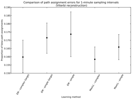
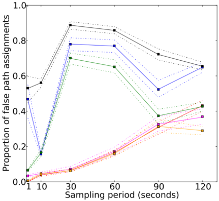
• The proportion of path misses: for each trajectory, it is the number of times the most likely path was not the true path followed, divided by the number of time steps in the trajectory.
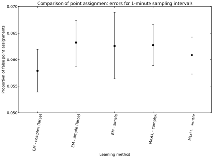
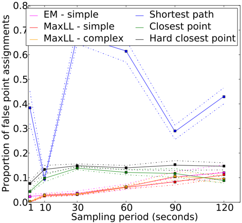
• The proportion of state misses: for each trajectory, the number of times the most likely projection was not the true projection.
• The log-likelihood of the true point projection. This is indicative of how often the true point is identified by the model.
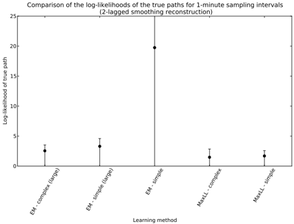
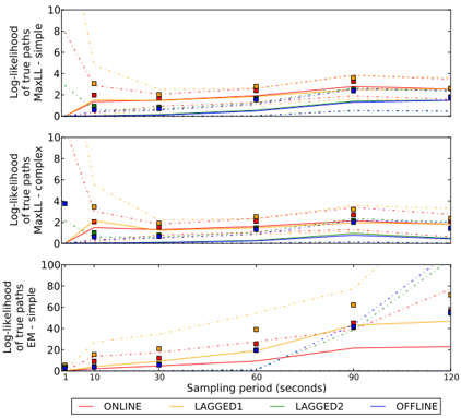
• The log-likelihood of the true path.
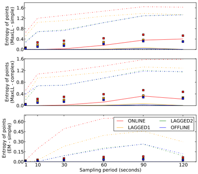
• The entropy of the path distribution and of the point distribution. This statistical measure indicates the confidence assigned by the filter to its result. A small entropy (close to 0) indicates that one path is strongly favored by the filter against all the other ones, whereas a large entropy indicates that all paths are equal.
• The miscoverage of the route. Given two paths p and p ′ the coverage of p by p ′ , denoted cov ( p, p ′ ) is the amount of length of p that is shared with p ′ (it is a semi-distance since it is not symmetric). It is thus lower than the total length | p | of the path p . We measure the dissimilarity of two paths by the relative miscoverage : mc ( p ) = 1 -cov ( p ∗ ,p ) | p ∗ | . If a path is perfectly covered, its relative miscoverage will be 0.

For about 0.06% of pairs of points, the true path could not be found by the A* algorithm and was manually added to the set of discovered paths

Each training session was evaluated with k-fold crossvalidation, using the following parameters:

Sampling rate (seconds)	Batches used for validation	Batches used for training
1	1	5
10	3	5
30	6	5
60	6	5
90	6	5
120	6	5

B. Results

Given the number of parameters to adjust, we only present the most salient results here.

The most important practical result is the raw accuracy of the filter: for each trajectory, which proportion of the paths or of the points was correctly identified? These results are presented in Figure 12 and Figure 13. As expected, the error rate is 0 for high frequencies (low sampling period): all the points are correctly identified by all the algorithms. In the low frequencies (high sampling periods), the error is still low (around 10%) for the trained models, and also for the greedy model ('Hard closest point'). For sampling rates between 10 seconds and 90 seconds, trained models ('Simple' and 'Complex') show a much higher performance compared to untrained models ('Hard closest point', 'Closest point' and 'Shortest path').

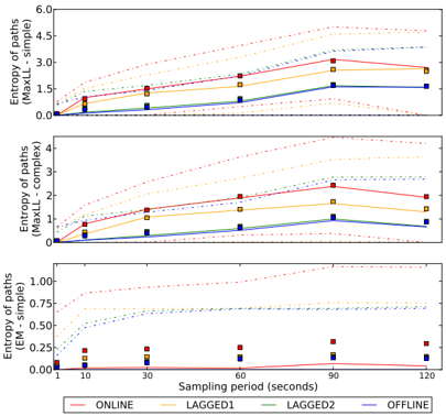
We now turn our attention to the resilience of the models, i.e. how they perform when they make mistakes. We use two statistical measures: the (log) likelihood of the true paths (Figure 14) and the entropy of the distribution of points or paths (Figures 15 and 16). Note that in a perfect reconstruction with no ambiguity, the log likelihood would be zero. Interestingly, the log likelihoods appear very stable as the sampling interval grows: our algorithm will continue to assign high probabilities

to the true projections even when many more paths can be used to travel from one point to the other. The performance of the simple and the complex models improves greatly when some backward filtering steps are used, and stays relatively even across different time intervals.

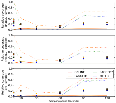
We conclude the performance analysis by a discussion of the miscoverage (Figure 17). The miscoverage gives a good indication of how far the path chosen by the filter differs from the true path. Even if the paths are not exactly the same, some very similar path may get selected, that may differ by a turn around a block. Note that the metric is based on length covered. At high frequency however, the vehicle may be stopped and cover a length 0. This metric is thus less useful at high frequency. A more complex model improves the coverage by about 15% in smoothing. In high sampling resolution, the error is close to zero: the paths considered by the filter, even if they do not match perfectly, are very close to the true trajectory for lower frequencies. Two groups clearly emerge as far as computing strategies are concerned: the online/1-lag group (orange and red curves) and the 2-lag and offline group (green and blue curves). The relative miscoverage for the latter group is so low that more than half of the probability mass is at zero. A number of outliers still raise the curve of the last quartile as well as the mean, especially in the lower frequencies. The paths inferred by the filter are never dramatically different: at two minute time intervals (for which the paths are 1.7km on average), the returned path spans more than 80% of the true path on average. The use of a more complicated model decreases the mean miscoverage as well as all quartile metrics by more than 15%.

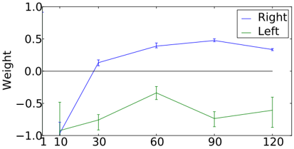
In the case of the complex model, the weights can provide some insight into the features involved in the decision-making process of the driver. In particular, for extended sampling rates (t=120s), some interesting patterns appear. For example, the drivers do not show a preference between driving through stop signs ( w 3 = -0 . 24 ± 0 . 07 ) or through signals ( w 4 = -0 . 21 ± 0 . 11 ). However, drivers show a clear preference to turn on the right as opposed to the left, as seen in Figure 18. This is may be attributed, in part, to the difficulty in crossing an intersection in the United States.

From a computation perspective, given a driver model, the filtering algorithm can be dramatically improved for about as much computations by using a full backward-forward (smoothing) filter. Smoothing requires backing up an arbitrary sequence of points while 2-lagged smoothing only requires the last two points. For a slightly greater computing cost, the filter can offer a solution with a lag of one or two interval time units that is very close to the full smoothing solution. Fixedlag smoothing will be the recommended solution for practical applications, as it strikes a good balance of computation costs, accuracy and timeliness of the results.

It should be noted the algorithm continues to provide decent

results even when points grow further apart. The errors steadily increase with the sampling rate until the 30 seconds time interval, after which most metrics reach some plateau. This algorithm could be used in tracking solutions to improve the battery life of the device by up to an order of magnitude for GPSs that do not need extensive warm up. In particular, the tracking devices of fleet vehicle are usually designed to emit every minute as the road-level accuracy is not a concern in most cases.

C. Unsupervised learning results

The filter was also trained for the simple and complex models using Dataset 2. This dataset does not include true observations but is two orders of magnitude larger than Dataset 1 for the matching sampling period (1 minute). We report some comparisons between the models previously trained with Dataset 1 ('MaxLL-Simple', 'EM-Simple', 'MaxLLComplex') and the same simple and complex models trained on Dataset 2: 'EM-Simple large' and 'EM-Complex large'. The learning procedure was calibrated using cross-validation and was run in the following way: all unsupervised models were initialized with a hand-tuned heuristic model involving only the standard deviation and the characteristic length (with

the weight of all the features set to 0). The ExpectationMaximization algorithm was then run for 3 iterations. Inside each EM iteration, the M-step was run with a single NewtonRaphson iteration at each time, using the full gradient and Hessian and a quadratic penalty of 10 -2 . During the E step, each sweep over the data took 13 hours 400 thousand points on a 32-core Intel Xeon server.

We limit our discussion to the main findings for brevity. The unsupervised training finds some weight values similar to those found with supervised learning. The magnitude of these weights is larger than in the supervised settings. Indeed, during the E step, the algorithm is free to assign any sensible value to the choice of the path. This may lead to a self-reinforcing behavior and the exploration of a bad local minimum.

As Figures 21, 23, and 22 show, a large training dataset puts unsupervised methods on par with supervised methods as far as performance metrics are concerned. Also, the inspection of the parameters learned on this dataset corroborates the finding made earlier. One is tempted to conclude that given enough observations, there no need to collect expensive highfrequency data to train a model.

D. Key findings

Our algorithm can reconstruct a sensible approximation of the trajectory followed by the vehicles analyzed, even in complex urban environments. In particular, the following conclusions can be made:

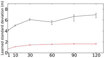
Figure 19. Standard deviation learned by the simple models, in the supervised (Maximum Likelihood) setting and the EM setting. The error bars indicate the complete span of values computed for each time. Note that the maximum likelihood estimator rapidly converges toward a fixed value of about 6 meters across any sampling time. The EM procedure also rapidly converges, but it is overconfident and assigns a lower standard deviation overall.

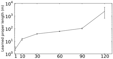
Figure 20. Characteristic length learned by the simple models, in the supervised (Maximum Likelihood) setting and the EM setting. As hoped, it roughly corresponds to the expected path length. The error bars indicate the complete span of values computed for each time (0th and 100th percentile). Note how the spread increases for large time intervals. Indeed, vehicles have different travel lengths at such time intervals, ranging from nearly 0 (when waiting at a signal) to more than 3 km (on the highway) and the models struggle to accommodate a single characteristic length. This justifies the use of more complicated models.

Figure 21. Expected likelihood of the true path. The central point is the mean log-likelihood, the error bars indicate the 70% confidence interval. Note that the simple model trained unsupervised with the small dataset has a much larger error, i.e. it assigns low probabilities to the true path. Both unsupervised models tend to express the same behavior but are much more robust.

• An intuitive deterministic heuristic ('Hard closest point') dramatically fails for paths at low frequencies, less so for points. It should not be considered for sampling intervals larger than 30 seconds.
• A simple probabilistic heuristic ('closest point') gives good results for either very low frequencies (2 minutes) or very high frequencies (a few seconds) with more 75% of paths and 94% points correctly identified. However, the incorrect values are not as close to the true trajectory as they are with more accurate models ('Simple' and 'Complex').
• For the medium range (10 seconds to 90 seconds), trained models (either supervised or unsupervised) have a greatly improved accuracy compared to untrained models, with 80% to 95% of the paths correctly identified by the former.

• For the paths that are incorrectly identified, trained models ('Simple' or 'Complex') provide better results compared to untrained models (the output paths are closer to the true paths, and the uncertainty about which paths may have been taken is much reduced). Furthermore, using a complex model ('Complex') improves these results even more by a factor of 13-20% on all metrics.
• For filtering strategies: online filtering gives the worst results and its performance is very similar to 1-lagged smoothing. The slower strategies (2-lagged smoothing and offline) outperform the other two by far. Two-lagged smoothing is nearly as good as offline smoothing, except in very high frequencies (less than 2 second sampling) for which smoothing clearly provides better results.
• Using a trained algorithm in a purely unsupervised fashion provides an accuracy as good as when training in a supervised setting - within some limits and assuming enough data is available. The model produced by EM ('EM-Simple') is equally good in terms of raw performance (path and point misses) but it may be overconfident.
• With more complex models, the filter can be used to infer some interesting patterns about the behavior of the drivers.

VI. CONCLUSIONS AND FUTURE WORK

We have presented a novel class of algorithms to track moving vehicles on a road network: the path inference filter . This algorithm first projects the raw points onto candidate projections on the road network and then builds candidate trajectories to link these candidate points. An observation model and a driver model are then combined in a Conditional Random Field to find the most probable trajectories.

The algorithm exhibits robustness to noise as well as to the peculiarities of driving in urban road networks. It is competitive over a wide range of sampling rates (1 seconds to 2 minutes) and greatly outperforms intuitive deterministic algorithms. Furthermore, given a set of ground truth data, the filter can be automatically tuned using a fast supervised learning procedure. Alternatively, using enough regular GPS data with no ground truth, it can be trained using unsupervised learning. Experimental results show that the unsupervised learning procedure compares favorably against learning from ground truth data. One may conclude that given enough observations, there no need to collect expensive high-frequency data to train a model.

This algorithm supports a range of trade-offs between accuracy, timeliness and computing needs. In its most accurate settings, it extends the current state of the art [43], [42]. This result is supported by the theoretical foundations of Conditional Random Fields. Because no standardized benchmark exists, the authors have released an open-source implementation of the filter to foster comparison with other methodologies using other datasets [1].

In conjunction with careful engineering, this program can achieve high map-matching throughput. The authors have written an industrial-strength version in the Scala programming language, deployed in the Mobile Millennium system. This version maps GPS points at a rate of about 400 points per second on a single core for the San Francisco Bay area (several hundreds of thousands of road links), and has been scaled to multicore architecture to achieve an average throughput of several thousand points per second [20].

A number of extensions could be considered to the core framework. In particular, more detailed models of the driver behavior as well as algorithms for automatic feature selection should bring additional improvements in performance. Another line of research is the mapping of very sparse data (sampling intervals longer than two minutes). Although the filter already attempts to consider as few trajectories as possible, more aggressive pruning may be necessary in order to achieve good performance. Finally, the EM procedure presented for automatically tuning the algorithm requires large amounts of data to be effective, and could be tested on larger datasets that what we have presented here.

Authors

Timothy Hunter is a Ph.D. student in the Department of Electrical Engineering and Computer Science and in the AMPLab, at the University of California at Berkeley. He received the Engineering Degree in Applied Mathematics from the Ecole Polytechnique,

France, in July 2007, and the M.S. degree in Electrical Engineering from Stanford University in 2009. His research interests include new programming models for Machine Learning with Big Data, and some applications to estimation and transportation.

Pieter Abbeel received a BS/MS in Electrical Engineering from KU Leuven (Belgium) and received his Ph.D. degree in Computer Science from Stanford University in 2008. He joined the faculty at UC Berkeley in Fall 2008, with an appointment in the Department of Electrical Engineering and Computer

Sciences. He has won various awards, including best paper awards at ICML and ICRA, the Sloan Fellowship, the Okawa Foundation award, and 2011's TR35. He has developed apprenticeship learning algorithms which have enabled advanced helicopter aerobatics, including maneuvers such as tic-tocs, chaos and auto-rotation, which only exceptional human pilots can perform. His group has also enabled the first end-to-end completion of reliably picking up a crumpled laundry article and folding it. His work has been featured in many popular press outlets, including BBC, MIT Technology Review, Discovery Channel, SmartPlanet and Wired.

Alexandre Bayen received the Engineering Degree in applied mathematics from the Ecole Polytechnique, France, in July 1998, the M.S. degree in aeronautics and astronautics from Stanford University in June 1999, and the Ph.D. in aeronautics and astronautics from Stanford University in December 2003. He was a Visiting Researcher at NASA Ames

Research Center from 2000 to 2003. He worked as the Research Director of the Autonomous Navigation Laboratory at the Laboratoire de Recherches Balistiques et Aerodynamiques, (Ministere de la Defense, Vernon, France), where he holds the rank of Major. He is an Associate Professor in the Electrical Engineering and Computer Sciences at UC Berkeley. Bayen has authored one book and over 100 articles in peer reviewed journals and conferences. He is the recipient of the Ballhaus Award from Stanford University, 2004, of the CAREER award from the National Science Foundation, 2009 and he is a NASA Top 10 Innovators on Water Sustainability, 2010. His projects Mobile Century and Mobile Millennium received the 2008 Best of ITS Award for Best Innovative Practice, at the ITS World Congress and a TRANNY Award from the California Transportation Foundation, 2009. Bayen is the recipient of the Presidential Early Career Award for Scientists and Engineers (PECASE) award from the White House, 2010. Mobile Millennium has been featured more than 100 times in the media, including TV channels and radio stations (CBS, NBC, ABC, CNET, NPR, KGO, the BBC), and in the popular press (Wall Street Journal, Washington Post, LA Times).

Acknowledgments

The authors wish to thank the staff at the California Center for Innovative Transportation, in particular Ryan Herring and Saneesh Apte, for their dedicated support. Discussions with Samitha Samarayanake have been instrumental in the writing this article. The authors are indebted to Warren Hoburg, and Kailin Kroetz for their thorough and insightful comments on the draft.

This research is supported in part by gifts from Google, SAP, Amazon Web Services, Cloudera, Ericsson, Huawei, IBM, Intel, Mark Logic, Microsoft, NEC Labs, Network Appliance, Oracle, Splunk and VMWare. The generous support of the US Department of Transportation and the California Department of Transportation is gratefully acknowledged. We also thank Nokia and NAVTEQ for the ongoing partnership and support through the Mobile Millennium project.

NOTATION

Symbol	Meaning
δ ( x, p )	Compatibility function between a state x and the start state of a path p
¯ δ ( p,x )	Compatibility function between an end state x and the end state of a path p
glyph[epsilon1] = σ - 2	Stacked inverse variance
η = η ( p | x )	Transition model
θ	Stacked vector of parameters
µ	Weight vector
ξ 1 , ξ 2	Simple features (path length and distance of a point projection to its GPS coordinate)
π	Probability distribution, the variables are always indicated to disambiguate which variables are involved
ˆ π	Probability distribution in the case of a dynamic Bayesian network, the variables are always indicated to disambiguate which variables are involved
˜ π	Expected plug-in distribution
ς	Set of valid trajectories
σ	Standard deviation
= x 1 p 1 x 2 ...p T - 1 x T	Trajectory of a vehicle
τ ∗	Most likely trajectory given a model ( ω, η ) and a GPS track g 1: T
φ ( τ | g 1: T )	Potential, or unnormalized score, of a trajectory
φ t i	Maximum of all the potentials of the partial trajectories that end in the state x t i
φ ∗	Maximum value over all the potentials of the trajectories compatible with g 1: T
ϕ ( p )	Feature function
ψ ( z 1: L )	Generalized potential function
ω = ω ( g | x )	Observation model
Ω( x )	Prior distribution over the states x
g	GPS coordinate (pair of latitude and longitude)
( g t ) 1: T	Sequence of all T GPS observations of a GPS track
I t	Number of projected states of the GPS point at time index t onto the road network
I	Number of mappings of the GPS point onto the road network
J	Number of all candidate trajectories between the mappings x and x ′
J t	Number of all trajectories between the mappings at time t (i.e. x t ) and the mappings at time t +1 x t +1
( l, o )	Location in the road network defined by a pair of a road link l and an offset position o on this link
L = 2 T - 1	Complete length of a trajectory
L	Expected likelihood
N = ( V , E )	Road network, comprising some vertices (nodes) N and edges (roads) E
x = ( l, o )	State of the vehicle (typically a location on the road network)
p	Path between one mapping x and one subsequent mapping x ′
p = ( p j ) 1:	Collection of all J candidate trajectories between a set of candidate states x and a subsequent set x
J p t = ( p t j ) 1: J t	Collection of all J candidate trajectories between the set of candidate states at time t x t and the subsequent set x t +1
¯ q t i	Probability that the vehicle is in the discrete state x t i at time t given all observations
- → q t i	Probability that the vehicle is in the discrete state x t i at time t given all observations up to time t
← - q t i	Probability that the vehicle is in the discrete state x t i at time t given all observations after time t +1
r t j	Probability that the vehicle uses the (discrete) path p t j at time t given all observations
- → r t j	Probability that the vehicle uses the (discrete) path p t j at time t given all observations up to time t
← - r t j	Probability that the vehicle uses the (discrete) path p t j at time t given all observations after time t +1
T	Number of GPS observations for a track
T l ( z l )	Generalized feature vector
Z	Partition function

REFERENCES

1. Supporting code for the path inference filter. https://github.com/tjhunter/ Path-Inference-Filter/.
2. A. Bayen, J. Butler, A. Patire, and et al. Mobile Millennium final report. Technical report, University of California, Berkeley, CCIT Research Report UCB-ITS-CWP-2011-6, 2011.
3. J. L. Bentley and H. A. Maurer. Efficient worst-case data structures for range searching. Acta Informatica , 13:155-168, 1980. 10.1007/BF00263991.
4. M. Bierlaire and G. Flötteröd. Probabilistic multi-modal map matching with rich smartphone data. In STRC 2011 , 2011.
5. M. Bierlaire and E. Frejinger. Route choice modeling with networkfree data. Transportation Research Part C: Emerging Technologies , 16(2):187-198, 2008.
6. J.A. Bilmes. A gentle tutorial of the EM algorithm and its application to parameter estimation for Gaussian mixture and hidden Markov models. International Computer Science Institute , 4, 1998.
7. S.P. Boyd and L. Vandenberghe. Convex optimization . Cambridge Univ Pr, 2004.
8. S. Brakatsoulas, D. Pfoser, R. Salas, and C. Wenk. On map-matching vehicle tracking data. In Proceedings of the 31st international conference on Very large data bases , pages 853-864. VLDB Endowment, 2005.
9. The Cabspotting program. http://cabspotting.org/.
10. Y. Cui and S.S. Ge. Autonomous vehicle positioning with gps in urban canyon environments. Robotics and Automation, IEEE Transactions on , 19(1):15-25, 2003.
11. A. Downs. Still stuck in traffic: coping with peak-hour traffic congestion . Brookings Inst Pr, 2004.
12. J. Du, J. Masters, and M. Barth. Lane-level positioning for in-vehicle navigation and automated vehicle location (avl) systems. In Intelligent Transportation Systems, 2004. Proceedings. The 7th International IEEE Conference on , pages 35-40. IEEE, 2004.
13. M.E. El Najjar and P. Bonnifait. A road-matching method for precise vehicle localization using belief theory and kalman filtering. Autonomous Robots , 19(2):173-191, 2005.
14. G.D. Forney Jr. The Viterbi algorithm. Proceedings of the IEEE , 61(3):268-278, 1973.
15. L. Giovannini. A Novel Map-Matching Procedure for Low-Sampling GPS Data with Applications to Traffic Flow Analysis . Universita di Bologna, 2011.
16. J.S. Greenfeld. Matching GPS observations to locations on a digital map. In 81th Annual Meeting of the Transportation Research Board , 2002.
17. F. Gustafsson, F. Gunnarsson, N. Bergman, U. Forssell, J. Jansson, R. Karlsson, and P.J. Nordlund. Particle filters for positioning, navigation, and tracking. Signal Processing, IEEE Transactions on , 50(2):425437, 2002.
18. P.E. Hart, N.J. Nilsson, and B. Raphael. A formal basis for the heuristic determination of minimum cost paths. IEEE transactions on Systems Science and Cybernetics , 4(2):100-107, 1968.
19. B. Hoh, M. Gruteser, R. Herring, J. Ban, D. Work, J. Herrera, and A. Bayen. Virtual trip lines for distributed privacy-preserving traffic monitoring. In The Sixth Annual International conference on Mobile Systems, Applications and Services (MobiSys 2008) , Breckenridge, U.S.A., June 2008.
20. T. Hunter, T. Moldovan, M. Zaharia, J. Ma, S. Merzgui, M. Franklin, and A. Bayen. Scaling the mobile millennium system in the cloud. In submitted to ACM Symposium on Cloud Computing , 2011.
21. Inrix Inc. http://www.inrix.com.
22. J. D. Lafferty, A. McCallum, and F. C. N. Pereira. Conditional random fields: Probabilistic models for segmenting and labeling sequence data. In Proceedings of the Eighteenth International Conference on Machine Learning , ICML '01, pages 282-289, San Francisco, CA, USA, 2001. Morgan Kaufmann Publishers Inc.
23. K. Liu, T. Yamamoto, and T. Morikawa. Study on the cost-effectiveness of a probe vehicle system at lower polling frequencies. International Journal of ITS Research , 6(1):29-36, 2008.
24. T. Miwa, T. Sakai, and T. Morikawa. Route identification and travel time prediction using probe-car data. International Journal , 2004.
25. T.K. Moon. The expectation-maximization algorithm. Signal Processing Magazine, IEEE , 13(6):47-60, 1996.
26. K. P. Murphy. Dynamic Bayesian Networks: Representation, Inference and Learning . PhD thesis, University of California at Berkeley, 1994.
27. NAVTEQ Inc. http://www.navteq.com.
28. W.Y. Ochieng, M. Quddus, and R.B. Noland. Map-matching in complex urban road networks. Revista Brasileira de Cartografia , 2(55), 2009.
29. J.S. Pyo, D.H. Shin, and T.K. Sung. Development of a map matching method using the multiple hypothesis technique. In Intelligent Transportation Systems, 2001. Proceedings. 2001 IEEE , pages 23-27. IEEE, 2001.
30. M.A. Quddus, W.Y. Ochieng, and R.B. Noland. Current map-matching algorithms for transport applications: State-of-the art and future research directions. Transportation Research Part C: Emerging Technologies , 15(5):312-328, 2007.
31. M.A. Quddus, W.Y. Ochieng, L. Zhao, and R.B. Noland. A general map matching algorithm for transport telematics applications. GPS solutions , 7(3):157-167, 2003.
32. D.L. Schrank, T.J. Lomax, and Texas Transportation Institute. 2009 Urban mobility report . The Texas A&M University, 2009.
33. K. Seymore, A. McCallum, and R. Rosenfeld. Learning hidden Markov model structure for information extraction. In AAAI-99 Workshop on Machine Learning for Information Extraction , pages 37-42, 1999.
34. S. Syed and ME Cannon. Fuzzy logic-based map matching algorithm for vehicle navigation system in urban canyons. In ION National Technical Meeting, San Diego, CA , volume 1, pages 26-28, 2004.
35. Telenav Inc. http://www.telenav.com.
36. A. Thiagarajan, J. Biagioni, T. Gerlich, and J. Eriksson. Cooperative transit tracking using smart-phones. In Proceedings of the 8th ACM Conference on Embedded Networked Sensor Systems , pages 85-98. ACM, 2010.
37. Arvind Thiagarajan, Lenin S. Ravindranath, Katrina LaCurts, Sivan Toledo, Jakob Eriksson, Samuel Madden, and Hari Balakrishnan. Vtrack: Accurate, energy-aware traffic delay estimation using mobile phones. In 7th ACM Conference on Embedded Networked Sensor Systems (SenSys) , Berkeley, CA, November 2009.
38. S. Thrun. Probabilistic robotics. Communications of the ACM , 45(3):5257, 2002.
39. C. Wenk, R. Salas, and D. Pfoser. Addressing the need for map-matching speed: Localizing global curve-matching algorithms. In Scientific and Statistical Database Management, 2006. 18th International Conference on , pages 379-388. IEEE, 2006.
40. C. E. White, D. Bernstein, and A. L. Kornhauser. Some map matching algorithms for personal navigation assistants. Transportation Research Part C: Emerging Technologies , 8(1-6):91-108, 2000.
41. D. Work, O. Tossavainen, S. Blandin, A. Bayen, T. Iwuchukwu, and K. Tracton. An ensemble Kalman filtering approach to highway traffic estimation using GPS enabled mobile devices. In Proceedings of the 47th IEEE Conference on Decision and Control , pages 5062-5068, Cancun, Mexico, December 2008.
42. J. Yuan, Y. Zheng, C. Zhang, X. Xie, and G.Z. Sun. An interactivevoting based map matching algorithm. In Mobile Data Management (MDM), 2010 Eleventh International Conference on , pages 43-52. Ieee, 2010.
43. Y. Zheng and M.A. Quddus. Weight-based shortest-path aided mapmatching algorithm for low-frequency positioning data. In Transportation Research Board 90th Annual Meeting , 2011.