Theoretical Foundations for Abstraction-Based Probabilistic Planning

Vu Ha

Department of EE &

University of { vu, haddawy} @cs. uwm. edu

Abstract

Modeling worlds and actions under uncer­ tainty is one of the central problems in the framework of decision-theoretic planning. The representation must be general enough to capture real-world problems but at the same time it must provide a basis upon which theoretical results can be derived. The cen­ tral notion in the framework we propose here is that of the affine-operator, which serves as a tool for constructing (convex) sets of prob­ ability distributions, and which can be con­ sidered as a generalization of belief functions and interval mass assignments. Uncertainty in the state of the worlds is modeled with sets of probability distributions, represented by affine-trees, while actions are defined as tree-manipulators. A small set of key proper­ ties of the affine-operator is presented, form­ ing the basis for most existing operator-based definitions of probabilistic action projection and action abstraction. We derive and prove correct three projection rules, which vividly illustrate the precision-complexity tradeoff in plan projection. Finally, we show how the three types of action abstraction identified by Haddawy and Doan are manifested in the present framework.

Keywords: Decision-theoretic planning, plan projection, action abstraction, convex sets of probability functions.

1 INTRODUCTION

In the framework of decision-theoretic planning (DTP), uncertainty in the state of the world and in the effects of actions are represented with probabili­ ties, and the planner's goals, as well as tradeoffs among them, are represented with utilities. Given this repre­ sentation, the objective is to find an optimal or near

*Thanks to AnHai Doan for helpful comments. This work was partially supported by NSF grant IRI-9509165.

Peter Haddawy· CS Wisconsin-Milwaukee optimal plan or policy, where optimality is defined as maximizing expected utility.

In most of the existing DTP approaches, the world is represented with a probability distribution over the state space, and actions are defined as stochastic map­ pings among the states [ 12 , 3, 1, 16]. Given this framing of the problem, all probabilistic and decision­ theoretic planners face the burden of computational complexity in seeking an optimal or near-optimal so­ lution. One popular way to address this problem is to use abstraction techniques to guide the search through the plan space and to reduce the cost of plan eval­ uation. This concept has been applied in Markov process-based planning [1] as well as less structured approaches [12, 9]. Because of the wide applicability of abstraction techniques in decision-theoretic planning, a simple and general theory of action abstraction that could form the basis for comparison of approaches and development of new approaches is desirable. This pa­ per attempts to provide such a theory.

This paper has its origins in the work of Hanks [12], Tenenberg [14], and Haddawy and Suwandi [ll), as well as later work by Doan and Haddawy [8, 9, 4, 5]. In the framework of Doan and Haddawy, the planning problem is formalized as the problem of searching for the optimal plan through the space of possible plans, each of which is a sequence of actions. The planner is armed with the capability of understanding and evalu­ ating abstract plans constructed from abstract actions, and thus is able to evaluate and eliminate a set of sub­ optimal plans without explicitly evaluating each mem­ ber of that set. The introduction of abstract actions, however, discards the conventional world and action representations. An abstract action is a function that maps a probability distribution to a set of probability distributions.

A mechanism for representing sets of probability func­ tions in this planning framework must satisfy the fol­ lowing requirements. First, it must be computation­ ally achievable; we cannot, for example, just explicitly list all the members of the set. Second, it must en­ able the planner to project actions, especially abstract actions on the worlds it represents. Third, since pro-

jecting an abstract plan will result in a set of prob­ ability functions, transforming the task of computing expected utilities to the task of computing expected utility intervals, algorithms to perform this task must be provided. And finally, the mechanism should sup­ port the process of abstracting actions and plans.

One of the first attempts at addressing the first two of the above four problems is the work of Chrisman [2]. Chrisman represents uncertainty by a set of prob­ ability functions that are consistent with a belief func­ tion, which in turn is represented by a basic proba­ bility function (or a mass assignment). He then pro­ vides a closed-form projection rule to project actions on this kind of set. Doan [4, 5] attempts to answer all of the four questions posted in the preceding para­ graph by introducing the notion of general or interval mass assignment (IMA), which is used as a representa­ tion for certain (convex) sets of probability functions. Although introduced as a generalization of belief func­ tions, IMAs are still not expressive enough; in order to derive a closed-form projection rule, we must sacrifice too much information and thus obtain weak approxi­ mations for the projected worlds.

In this paper, we address the above problems by intro­ ducing t h e affine-operator, which is used to construct (convex) sets of probability functions, including (Theo­ rem 1) IMAs and belief functions as special cases. The worlds are represented as affine-trees, which dynami­ cally grow with the advancing of the projection pro­ cess. Actions are categorized as primitive -mapping probability functions to probability functions, and ab­ stractmapping probability functions to sets of prob­ ability functions.

The rest of this paper is organized as follows. In Sec­ tion 2.1, we define the affine-operator, affine-trees, and the class of affine-worlds. The heart of our framework is a small set of lemmas investigating the properties of affine-trees and is presented in Section 2.2. We present the action model in Section 3. Three projection rules are presented and shown to be correct in Section 4 (Theorem 2). The projection rules are descending in term of precision but ascending in term of practical usefulness. The problem of computing the expected utility interval is solved by an efficient algorithm sug­ gested by Theorem 3 in Section 5. In Section 6, we revisit the three abstraction techniques identified by Haddawy and Doan and prove them correct (Theorem 4). We then conclude and discuss future research in Section 7. Due to space limitations, proofs of several theorems are only sketched or omitted. The complete proofs, as well as additional discussion can be found in [7].

Terminology and Notation. We will use the follow­ ing notations throughout the paper. A state s repre­ sents a possible complete description of all information relevant to the planner. The set of all such descriptions is call the state space (denoted n) and is assumed to be finite. A world w is the uncertain knowledge the plan- ner actually has at a certain time point, which can be either (i) a state s E r2 (no uncertainty, deterministic world), (i i ) a Bayesian 1 probability distribution over the state space n (probabilistic world), or (iii) a set of such probability distributions ( ge n er a l world). The set of all probabilistic worlds is denoted by !J, and thus the set of all general worlds can be denoted by 2 P. The above three classes of worlds form a chain in which each element is a strict superset of its preced­ ing element: n c p c 2P. For the sake of simplicity, the interpretation of a world (a state, a PD, or a set of PDs) will be left implicit in the discussion where misunderstanding can be excluded. A world w1 E 2P is said to subsume a world w2 E 2P if w1 2 w2. The convex hull of a world w E 2P, denoted by CH( w ) is defined to be the smallest world that contains w and all convex combinations 2 of elements of w. A world w is said to be convex, if w = CH(w).

We will be performing operations on intervals. Every interval is assumed to be an (open or closed) subinter­ val of the interval [0, 1]. The set of all such intervals is denoted by Q. Operations on the intervals such as addition, multiplication, etc. are defined in the obvi­ ous way. For example, the multiplication of two in­ tervals [1 1 , ul ) and [12, u2] is defined to be the interval [/1./2 , ul.u2). The lower and upper bound of an inter­ val Q are denoted by L( Q) and U ( Q), respectively.

2 THE AFFINE-OPERATOR AND AFFINE-WORLDS

2.1 BASIC DEFINITIONS

We first introduce the notion of affine-vectors. Any vector whose components are numbers between 0 and 1 and sum up to 1 is called an affine-vector 3. The central notion of our framework is the notion of the affine-operator, defined as follows.

Definition 1 (The Affine-Operator ) The

affine operator defined by an n-dimenszon affine-vector if= ( q1, q2, ... , qn) is the function that maps any vec­ tor P = (P1, P 2 , . . . , Pn) E pn of probability functwns to the probability function R =if® P := 2:::7=1 q;P;.

It is not hard to see that the above definition is correct, i.e., R is indeed a probability function. We extend the affine operator, "®" to deal with vectors of intervals and vectors of worlds as follows.

1 Bayesian probability distributions are probability func­ tions that assign a probability number to every single ele­ ment of the sample space (which in this case is 0).

2 A convex combination of n probability functions P1, P2, ... , Pn is a probability function of the form L�-I a,P,, where 0 � /J'i � 1 and L�=l a, = 1.

3 The "affine" term comes from the similar terminology used in linear algebra.

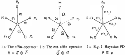
R=q®P

CH('fJ')

Figure 1: The affine-operator and examples

Definition 2 (The Extended Affine-Operator) The affine-operator defined by an n-dimension interval vector Q = (Q1, Q2, . . . , Qn) E gn is the function that maps any world vector w = ( w1, w2, ... , wn ) E (2�-') n to the world Q @ w that is the set of all probability functions of the form q@ P, where if= ( qt, qz , ... , qn) is any affine-vector such that q; E Q;, and P = (Pt, P2, ... , Pn) is any vector of probability functions such that P; E w;, for all i = 1, 2, . . . , n.

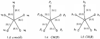
Henceforth, the term affine-operator will be used to refer to the extended definition. The probability func­ tion R = q@P a n d the world Q@w can be represented by a center of a star S with n branches (and thus n leaves) (Figures La and 1. b). The branches are asso­ ciated with the n u m bers q; and intervals Q;, while the leaves are a s soc i at ed with probability functions P; and the worlds w;, i = 1, 2, ... , n, respectively. We will call a star whose branches are associated with intervals an affine-star. Thus, every affine-star will define exactly o n e a ffi n e -op er ator.

Example 1. We first notice that any Bayesian proba­ bility function P can be represented by an lfll-branch affine-star (Figure l.c). The leaves of this star are as­ sociated with the states b E n, and the branches are associated with the probability numbers P( b).

Example 2. Consider the case where each branch Q; is the entire interval [0, 1] (Figures l.d, l.e, l.f). The corresponding affine-operator will create the con­ vex combinatzon of the leaf-worlds Wt, w2, . . . , Wn, de­ noted by conv ( w1,w2, . . . , wn ) , or conv(w) (Figure l.d). When each world w; is a single probability func­ tion P;, the world conv( P1, Pz, ... , Pn) is exactly the conventional convex hull of the set of probability func­ tions P = {P1,P2, . . . ,Pn}, CH(P) (Figure l.e). In the more special case, where each probability func­ tion P; is a state b;, with B = { b1, bz, .. . , bn}, th e convex hull of B, CH(B) ( Figure l.f ) is the set of all probability functions that assign p o s i t i v e proba­ bility to only the elements of B. Notice that the function that maps any set of states B to the world CH(B) is monoton increasing, i.e., CH(B) C CH(C) iff B C C. In particular, CH(fl) = p. Furthermore, conv(CH(B), CH(C)) = CH(B U C).

Sometimes it can be the case that in an affine-star some of the leaf-worlds w; are also worlds constructed by using the affine operator, and are represented by other affine-stars. This observation gi v e s rise to the notion of affine-trees. A tree whose branches are as­ sociated with intervals is called an affine-tree. Affine­ stars are thus special affine-trees with depth 1.

When the leaves of an affine tree T are associated with worlds, then each node N ofT will be associated with the world obtained by applying the affine operator re­ cursively on the subtree ofT that has N as its root. An affine-tree thus defines the composition of a sequence of affine-operators (or affine-stars).

Within the class of worlds that can be represented by affine-trees, we define the following class of worlds.

Definition 3 (Affine-Worlds) The class of affine­ worlds, denoted by A:F:F, is the set of all worlds that can be represented by an affine-tree whose leaves are associated with states.

If w is an affine-world represented by an a ffi ne -t r e e T whose leaves are associated with states, then T is called a standard affine-tree of w. From Examples 1 (Figure l.c), we know that any probability function is an affine-world having a standard affine-tree with depth 1. Example 2 (Figure l.f) tells us that for any B � !1, CH(B) also has the same p r operti es . The following theorem says that belief fu n c t i o n s [13], when interpreted as sets of probability functions, are also affine-worlds having standard affine-trees of depth 2.

Theorem 1 (Belief functions Are Affine-Worlds) Let Bel be a belief function with the corresponding ba­ sic probability function (mass assignment) m. Denote the focal element of m by B1, B2, . .. , En. Then the set of probability functwns that are consistent 4 with Bel is an affine-world represented by an n-branch affine­ star with branches m(B;) and leaves CH(B;).

In [4, 5], belief functions, by means of mass assign­ ments, are generalized to interval mass assignments by allowing mass functions to be interval-valued. It i s clear that interval m as s ass i g nme nts are affine-worlds represented by affine-stars with interval-branches and leaves of the form CH(B), B � n.

4 A probability function P is consistent with a belief function Bel if Bel( B):::; P(B), VB� 0.

2.2 LEMMAS

In this section, we present a set of lemmas concerning the affine-operator that form the heart of our frame­ work. In the rest of the paper, the leaves of any affine­ tree will be assigned worlds. In order to make the discussion less cumbersome, we shall not always dis­ tinguish a branch of an affine-tree from the interval associated with it, or an affine-tree from the world it represents, when doing so does not introduce ambigu­ ity. For example, the sentence "affine-tree T1 subsumes affine-tree T2" should be interpreted as meaning that the world represented by T1 subsumes the world rep­ resented by T2.

Lemma 1 (Monotonicity Lemma) Replacing any leaf-world with a subsuming world, or any branch­ interval with a subsuming interval in an affine-tree will result in a subsuming affine-tree.

Lemma 2 (Star-Merging Lemma) Consider a set of affine-stars { Si lj E J} having the same number n of branches. If S is an n-branch affine-star whose branch­ interval (respectively leaf-world} number i subsumes branch-interval {respectively leaf-world} number i of each Sj, 'Vj E J, 'Vi= 1, 2, . . . , n, then S 2 Sj, 'Vj E J.

Lemma 3 (Branch-Merging Lemma) Let S be an affine-star with n branches Q; and n leaves w;, and J � { 1, 2, . . . , n } . If S' is the affine-star obtained from S by "merging" branches index j E J to a single branch L: iE l Qi with the corresponding leaf conv(wilj E J), then S' 2 S.

Lemma 4 (Tree-Flatening Lemma} Let T be an affine-tree. IfT' is the tree obtained by ''jlatening" T, i.e., by replacing every path from the root r to a leaf l with a single branch associated with the multiplication of the branches along this path, then T' 2 T.

Lemma 5 (CH Invariance Lemma) Let S be an affine-star with n branches Q; and n leaves w;, i.e. S = Q 0 w. Then CH(S) = Q 0 CH(w) 5, where CH(w) = (CH(wt), CH(w2), . .. , CH(wn)).

Corollary 1 C H(w) = w, 'Vw E AF:F. As a con­ sequence, affine-worlds are convex sets of probability functions.

3 ACTION MODEL

3.1 PRIMITVE ACTIONS

A primitive action >. is a function mapping states into probability distributions over states: >. : n -+ p, and is represented by a finite set of tuples { < C;, p;, e; >I i} called branches. In each branch i, C; is a set of states, called the condition, p; is a number in [0, 1], called

5Thanks to Vu Ha Van for proving the � direction.

the probability, and e; is a function mapping states into states, called the primitive effect of action ..\. The conditions C; must be jointly exhaustive, i.e. their union i s n. The semantics of action ..\ is that it maps a state b E Q into a probability function >.(b) := Pb E r defined as: Pb(a) = 2:::; bEC ,;e;(b)=a Pi, 'ri a E 0 .

This semantics definition means that if the world be­ fore the execution of action..\ i s b, then for each branch index i whose condition satisfies b, the world after the execution of .>. will be e; ( b ) with probability p;. It is clear that this semantic definition is correct only if for all b E Q, the probabilities Pb( a ) for all a E Q sum to 1. By introducing the n o t i o n Sb ( C;) = 1 if C; 3 b and Sb(C;) = 0 otherwise, this condition is equivalent to

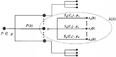
The probability function ..\(b) = Pb can then be repre­ sented by an n-branch affine-star whose branches are Sb(C;).p; and whose leaves are e;(b), i = 1, 2, . .. , n (see Figure 2, the dash-lined ellipse). We extend action .>. (which is a n _,. r function), to a r -+ r function as follows:

It is not hard to see that .>.( P) is indeed a probabil­ ity function represented by a 2-level affine-tree (Figure 2). In some similar frameworks, a probabilistic ac­ tion is represented by a set of mutually exclusive and jointly exhaustive conditions [12, 1 1] or discriminants [ 1]. Each condition is then associated with a finite set of probability-effect pairs, where the sum of the prob­ abilities is 1. An action in our framework can easily be transformed to this form 6. Here we adopt this representation because it facilitates a natural gener­ alization of primitive actions into abstract actions, as soon shown.

3.2 ABSTRACT ACTIONS

An abstract action A is a function mapping worlds into worlds: A : 210 -+ 2P, and is represented by a finite set of tuples { < C;, P;, E; >I i}, where the C; are jointly exhaustive conditions, the P; are subintervals of [0, 1], and the E; are functions mapping states into sets of states and are called abstract effects. In order to define the semantics of abstract actions, we first introduce the notion of effect and action instantiation.

6 Define a binary relation ,...., on the state space !1 such that Va, b E 0 : a "' b iff a and b a re satisfied by exactly the same set of conditions C;. Clearly, "" is an equiva­ lence relation on !1. The partition of !1 that corresponds to the factorization of 0 according to .-... will then give us a collection of mutually exclusive and jointly exhaustive con­ ditions. We can then reorganize the branches of the action according to these new conditions, obtaining the desired representation.

A primitive effect e is called an instantiated effect of an abstract effect E (denoted e E E) if for all s E 0, we have e(s) E E(s). A primitive action >. = { < C;, p;, e; >I i} is called an instantiated action of an abstract action A = { < C;, P;, E; >I i} (denoted ). E A) if p; E P; and e; E E; for each branch i. Note that the conditions C; of the instantiated action are the same as those of the abstract action. Primitive action ). , of course, must satisfy condition ( 1).

We are now in position to define the semantics of ab­ stract actions. An action A is a function that maps any world w E 2"' into the world

Abstracting actions has long been a popular method to cope with the complexity of planning in large prob­ lem spaces. The models for abstract actions, how­ ever, are diverse, and we have not seen any work that models abstract actions as functions operating on sets of probability functions. In the MDP framework of Boutilier and Dearden [1], concrete states are clustered into abstract states according to a set of relevant at­ tributes, and abstract actions are stochastic mappings among abstract states. In this sense, abstract actions are primitive actions wrt the abstract state space. In the work of Doan [4, 5], abstract actions do not have explicit semantics but are associated with projection rules. Defining actions as suggested in this paper offers some advantages in deriving procedures for abstract­ ing actions, as we shall see later.

4 ACTIONS ON AFFINE-WORLDS

Lemma 6 (Action Semi-lnvariance Lemma) Let Q E Q n be an n-dimension vector of intervals and w E (2�")n be an n-dimension vector of worlds and A be an action. Let A( w) = (A( wl ) , A( wz ) , . .. , A( wn)) . Then A(Q 0 w) c;;; Q 0 A(w).

The Action Semi-Invariance Lemma validates a classi­ cal use of the "divide and conquer" technique in pro­ jecting actions, provided that the pre-action world can be represented by an affine-tree. To be more specific, let us consider a pre-action world represented by an affine-tree T. If we replace every leaf-world l of the tree T with the world A(l), then the resulting affine­ tree will represent a world that subsumes A(w).

In the rest of the discussion, we shall assume that A is an action that has n branches: A = {(C;, P;, E;)li = 1,2, . . . , n } , and wE A:F:F is an affine-world repre­ sented by an affine-tree T( w ) . When T( w ) is in the standard form, i.e., the leaves of T( w) are associated with states, then we can project action A on w by re­ placing every leaf-state b with the world A(b). This is exactly the way the first projection rule works.

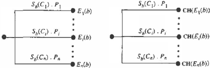
Projection Rule 1 (PRl) For every leaf b E 0 of the affine-tree T(w), we create an affine-star T1(A, b) (Figure 3, left) having n branches (leaves). The branches are associated with the intervals sb ( C; ).P; I while the leaves are associated with the worlds E;(b). The projected world is represented by the affine-tree T1 (A, w ) , which is obtained from T( w) by replacing ev­ ery leaf b with the corresponding affine-star T1(A, b).

It is clear that if each leaf-world E;(b) of the affine­ stars T1 (A, b) is a singleton state (for example, if the E; are primitive effects), then the projected world T1 (A, w ) is also an affine-world. This will no longer be true if some effect E; maps a state b into a set of at least two states. In other words, PRl, in general, is not closed on the class of affine-worlds, A:F:F. In order to obtain a closed-form projection rule, we have to trade some precision Notice that the hest affine­ approximation of a world B c;;; 0 is its convex hull, CH(B). This observation leads us to the second pro­ jection rule.

Projection Rule 2 (PR2) Same as PRl, except that T1(A, b) is replaced by T2(A, b) (Figure 3, right) whose leaves are associated with CH(E;(b)) instead of E;(b). The resulting affine-tree is denoted by T2(A, w ) .

Note that according to the CH Invariance Lemma, we have that T2(A, w) is exactly the convex hull of T1(A, w ) , from which the correctness ofPR2 is implied. Compared to PRl, PR2 gives a looser but more "rep­ resentable" result. By forcing the projected worlds to always be affine-worlds, the projection process can continue with more and more actions, "growing" a pro­ jection tree with more and more levels and leaves. This corresponds to the well-known forward projection al­ gorithm for probabilistic actions [12]. The next ques­ tion then arises: What is the complexity of this pro­ cess? The complexity of an affine-tree T is estimated (in this discussion) by two factors: the number of the levels (or the depth) ofT, denoted by D(T), and the number of the leaves ofT, denoted by £(T).

Recall that in PR2, we replace every leaf b with an affine-star having n leaves CH(E;(b)), i = 1, 2, .. . , n (see Figure 3, right). In order to apply PR2 to an­ other action, we have to standardize T2(A, w ) , which amounts to standardizing CH(E;(b)), for every leaf b of T(w) and i = 1, 2, ... , n. It is then clear that after

each action projection, the standard affine-tree repre­ se n ti n g the cu r r ent world will have two more levels: D(T2(A, w)) = D(T(w)) + 2. Fur t her m o re, if, on av­ erage, an abstract effect f u n c tio n E; maps a state into a set of k states, then, on average, t he number of the leaves of the current tree will increase by the factor of n x k: .C(T2(A,w)) = n x k x .C(T(w)).

In order to make the projection process less complex, we have to trade some more precision. The third pro­ jection rule is devised with this goal in mind. In the third projection rule, we do not require that any affine­ tree be standardized: it i s sufficient to make sure that the leaves of the affine-trees be associated with worlds of the form CH(B), B <,;:; n. We first introduce the following notation. For B, C <,;:; n, let SB(C) = 1 if C 2 B, 0 if C n B = 0, and [0, 1] otherwise.

Projection Rule 3 (PR3) For each leaf CH(B) of the affine-world T( w), we create an affine-star T3(A, CH(B)) {Fzgure 4.e) that has n branches (leaves). The branches are associated with the inter­ vals SB(C;).P;, while the leaves are associated with the worlds CH(E;(B n Ci)), i = 1, 2, ... , n. The affine-tree T3(A, w) is obtained from T( w) by replacing every leaf CH(B) with the corresponding affine-star T3(A, CH(B)).

It Is clear that D(T3(A, w)) = D(T(w)) + 1 and .C(T3(A, w )) = n x .C(T( w)). Thus, in a projection p r o ­ cess using PR3, after each action projection the num­ ber of the levels of the current affine-tree will increase by one, and the number of its leaves will increase by the factor of n, the n um b e r of the branches of the cur­ rently projected action. Furthermore, unlike the first two projection rules, PR3 essentially operates on sets of states instead of states, and thus is more tractable in cases of state spaces with large numbers of states. The following theorem p r o ve s the correctness of PR3.

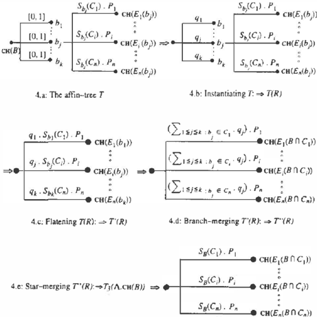
Theorem 2 (The Correctness Theorem)

For any action A and affine-world w, T3(A, w) is also an affine-world and T3(A, w) 2 T2(A, w) (and thus = CH(T1(A,w)) 2 CH(A(w)) 2 A(w)).

Proof:( Sketch) The first part of the theorem is triv­ ial. To prove the second part, it is sufficient to show that T3(A, CH(B)) 2 T2(A, CH(B)), for any B = {h,b2, ... ,bk } C 0. The main idea of the proof is the following. We start with the affine-tree T2(A, CH(B)) ( Fi gu re 4.a) and perform various op­ erations on it (Figures 4.b-e). After each operation (except the first one), the new affine-tree will subsume the old one, according to the lemmas in Section 2.2.

The first operation is instantiation: we instantiate T2(A, CH(B)) by t a k i ng a T2(A, R) affine-tree, where R E CH(B). Denote this tree by T(R) (Figure 4 . b ) . We then tree-fl.aten T(R), obtaning T'(R) (Figure 4.c), branch-merge T'(R) (according to each index i), ob­ t a i ni ng T"(R) ( F i g u r e 4.d). Finally, we st a r -m e r g e T"(R) for all R E CH(B), a n d use the o b s erv a t i o n that l:1::;i::;k bjEC; R ( b i ) E SB(C;), VR E CH(B) to obtain the final affine-tree T3(A, CH(B)) ( F i g u r e 4.e ) , c o m p l e t in g the proof (by the Monotonicity Le m ma ) . 0

Chrisman [2] provides a closed-form projection rule that works for probabilistic actions and w o r l ds that can be represented by belief f u nctio n s (or mass assign­ ments ) . The action representation is a special case of our representation, and thus his result is a l s o a special case of our result, namely PR3. Doan [5] uses IMAs to r e p r es e n t worlds and gives a proj e c t i on rule that differs from PR3 in that the projected affine-tree is al­ ways flatened to an affine-star. A comparison of these two rules is discussed in Section 7.

5 Computing the EUI of Affine-Worlds

Computing the expected utility of a plan is one of the most frequently performed oparations of a DTP plan­ ner. The upcoming theorem shows that computing the expected utility of affine-worlds can be done ele­ gantly, a g a i n using affine-trees as decompisition tools.

We first define the notion of utility function. A func­ tion f : Q __,. R is called a utility function. The ex­ pected utility of a world w E 2P is the set of real num­ bers defined as EU(w) = U:::sEQ P(s).f(s)IP E w}. The expected utility interval of w, denoted by EU I(w) is defined to be the convex hull 7 of EU ( w).

Theorem 3 (Affine-Worlds Utility Theorem) For all affine-world wE A:F:F, EU(w) = EUI(w).

Pr-oof:(Sketch) We prove this theorem using structural induction. Let w be an affine-world represented by a standard affine-tree T. Clearly, for any leave-state s ofT, we have EU I(s) = EU(s). Suppose now that for every node C ( C = child) on the rth level of T, we have computed EU I( C) and EU (C) = EU I( C). Then computing the EUI of any node P ( P =parent), (i.e., the lower and the upper bounds of the interval EU I ( P)) on the ( r - 1 )st level is a special instance of the knapsack problem, which can be efficiently solved using the greedy algorithm 8. It is also not hard to see that since EU( C) = EU I( C) for every child C, we will get EU(P) = E U I(P) for parent P . D

6 Abstracting Actions

In exchange for some loss of information, the Third Projection Rule provides a relatively simple method to approximate the post-action world by a subsum­ ing affine-world. The problem of projecting a plan, i.e. a sequence of actions, on an affine-world can then be solved by sequentially applying PR3 to each action in the plan, yielding a final affine-world w' that sub­ sumes the actual final world w. The expected utility interval of the actual final world, EU I( w) can then be bounded by EU I( w'), the EUI of the approximat­ ing affine-world, which can be efficiently computed us­ ing the recursive greedy knapsack algorithm (see the Affine-Worlds Utility Theorem). A plan can be elim­ inated if its expected utility interval is dominated by that of another plan.

The complexity of the process of evaluating and elimi­ nating suboptimal plans depends mainly on three fac­ tors: (i) the number of the branches of the actions in a plan, (ii) the number of the actions in a plan, and (iii) the number of alternative plans in the plan space. Three abstraction techniques are discussed in [6] to reduce the complexity of the planning pro­ cess. The intra-action abstraction technique, initially

7The convex hull of a set of real numbers is the smallest interval that contains all the numbers.

8The problem can be interpreted as the problem of packing objects of different values into a knapsack with fixed size ( l) such that the total value is minimized (for the lower bound) or maximized (for the upper bound). This algorithm is from Doan [5, 4]. The greedy knapsack al­ gorithm is also called the annihilation/reinforcement alg o ­ rithm by Tessem [15], who calls the minimizing step anni­ hilation, and the maximizing step reinforcement.

introduced by Hanks [12 ] who calls it bundlmg, re­ duces the branching factor of actions by replacing a set of branches by a single branch. We can use the Branch-Merging Lemma to apply this technique in our framework to produce correct abstractions. The sequential-action abstraction technique is used to re­ duce the length of a plan by replacing a subsequence of actions in that plan by a single action. We can use the Tree-Flatening Lemma to produce correct sequential abstractions. The inter-action abstraction technique, suggested by Tenenberg [14] is used to reduce the num­ ber of alternative plans in the plan space by grouping a set of actions (respectively plans) into a single ac­ tion (respectively plan). We can use the Star-Merging Lemma to produce correct inter-action abstractions.

Before presenting the abstraction procedures within our framework, the notion of correct abstraction needs to be clarified. Action abstractions can be correct with respect to different projection rules. An abstract ac­ tion A · is called a correct inter-abstraction of a set of actions { A1, A2, ... , A n } with respect to the projection rule number j, (j = 1,2,3) if 1j(A*,w) 2 7j ( A ;, w) , for all w E A:F:F and i :;:;: 1, 2, . . . , n. The correct­ ness criteria for intra- and sequential-action abstrac­ tions are defined similarly (see [7] for more details). Since plans cannot be projected with PR 1, we can only define the correctness of abstract plans wrt to PR2 or PR3. An abstract plan pl is a correct inter-abstraction of a set of plans {p/1, p/2 , ... , pln} wrt to projection rule number j (j = 2,3), ifTj(pl,w) 2 pl;(w), for all wE A:F:F and i = 1, 2, . . . , n.

It is not hard to see that an abstract plan that is built upon abstract actions that are correct wrt to a partic­ ular projection rule is correct wrt a looser projection rule. The problem here is to choose a projection rule to define the correctness criterion such that as-tight­ as-possible abstraction procedures can be derived. As the result of a careful analysis, we conclude that the Second Projection Rule is the best for this purpose 9. Due to space limitation, the full analysis of this prob­ lem is omitted here. Below we give the descriptions of the three abstraction procedures. The details are given in [7].

The three abstraction procedures are completely spec­ ified by three operators: bundle-branches, combine­ branches, and compose-branches, respectively. Each of these operators takes as arguments two branches 10 < C1, P1, E1 > and < C2, P2, E2 > and produces a single branch < C*, p·, E* >. The specification of < C*, P*, E* > for each operator is given below. We define the union of two effects E1 and E2 to be the function E1 U E2(s) = E1(s) U E2(s), and the compo­ sition of E1 and E2 to be the function (E2 o El)(s) =

9lntuitively, the reason for this is the fact that PRl pro­ duces non-convex sets, while PR3 is looser than PR2.

10It is straightforward to generalize these abstraction procedures to the case of grouping more than two branches (or actions).

Ue2EE2;e1EE1 e2 ( e 1 ( s ) ) .

• bundle-branches (for the intra-action abstraction procedure): C* C1 u C2, E* E1 U E2, and p· = PI + p2 if cl = c2 a n d [min{L(P1), L(P2)}, U(PL) + U(P2)] otherwise.
• combine-branches (for the inter-action abstraction procedure) : C* = C 1 U C2, E* = E1 U E 2 , and P* = [min{L(Pl), L(P2)}, max{U(PL), U(P2)}] if C1 = C2 and [0, max { U( Pl) , U(P2)}] otherwise.
• compose-branches (for the sequential-action ab­ straction procedure) : C* = cl n {b E n I El (b) n c2 =f 0} , E* = E2 0 El ' and P * = pl X p2.

Theorem 4 The above action abstraction procedures are correct with respect to the Second Projection Rule.

7 Related Work and Future Research

The affine-world representation in our framework has several advantages over the interval mass assignment representation of Doan [4, 5] . First, the affine-world representation is more general than the IMA represen­ tation; an IMA can be represented as a 2-level stan­ dard affine-tree, or a 1-level affine-star with leaves of the form C H (B) (Theorem 1). During the process of projecting actions on an IMA, the post-action world must be approximated with an IMA obtained from flatening the projected affine-tree, incurring a loss of information which can be significant in some extreme cases. One may think that this loss of information is traded for some gain of simplicity (a 1-level tree, in­ stead of a multi-level tree with the same number of leaves) , but it is not the case for two reasons. First, maintaining a multi-level tree T is not much more complex than a 1-level tree (star) S with the same number of leaves. For example, if, on average, each node of T has k children, then, on average, the ratio of the total number of the nodes in T to that i n S is: (l::�=O ki)/( 1 + kr ) :::: kj(k 1), which approaches 1 if k is large 1 1 . Second, since evaluating a plan often involves computing the utility of an entire chronicle [ 10] , the planner in the IMA framework must asso­ ciate each world in a chonicle with a separate IMA ( 1-level affine-tree), while the planner in our frame­ work can comfortably encode the whole chronicle in a single multi-level tree.

Haddawy et al [9] have implemented the DRIPS p l a n ­ ner, which uses the abstraction concepts discussed in this paper to construct and evaluate abstract plans. The DRIPS planner has been successfully applied to a number of real-world planning domains. The prob­ lems of estimating the loss due to abstraction and au­ tomatically generating abstraction hierarchies however remain quite difficult and challenging, and will form a main direction for our future work.

11 Here we do not consider extreme cases such as the case when T is a path. Flatening trees like this does not incur information loss.

References

1. C. Boutilier and R. Dearden. Using abstractions for decision-theoretic planning with time constraints. In Proceeding of the Twelfth National Conference on A r­ tificial Intelligence, pages 1 0 1 6- 1 022, Seattle 1 994.
2. L. Chrisman. Abstract probabilistic modeling of ac­ tion. In Proceeding of the First International Confer­ ence on Artificial Intelligence Planning Systems, 2836, June 1992.
3. T. Dean, L. Pack Kaelbling, J Kirman, and A. Nichol­ son. Planning with deadlines in stochastic domains. In Proceeding of the Eleventh National Conference on Artificial Intelligence, pages 574-579, July 1993.
4. A. Doan. Modeling probabilistic actions for practi­ cal decision-theoretic planning. In Proceeding of the Third International Conference on A I Planning Sys­ tems, May 1996. To appear
5. A. Doan. An abstraction-based decision-theoretic planning approach for partially observable metric do­ mains. Master Thesis UWM 1995.
6. A. Doan and P. Haddawy. Sound abstractions of prob­ abilistic actions in the constraint mass assignment framework. In Proceeding of the Twelfth Conference on Uncertainty in Artificial Intelligence, 1996.
7. V. Ha and P. Haddawy. DSAIL Technical Report TR01-03-96, Dept. of EE&CS, University of Wisconsin­ Milwaukee, March 1 996. Available at ftp.cs. uwm.edu in /pub/tech_reports/ai.
8. P. Haddawy and A. Doan. Abstracting probabilistic actions. In Proceeding of the Tenth Conference on Uncertainty in A rtificial Intelligence, pages 270-277, Seattle, July 1994.
9. P. Haddawy, A. Doan, and R. Goodwin. Efficient decision-theoretic planning: techniques and emprical analysis. In Proceeding of the Eleventh Conference on Uncertainty in Artificial Int e l l ig e n c e , pages 229-236, Montreal, August 1995.
10. P. Haddawy and S. Hanks. Representations for decision-theoretic planning: utility functions for dead­ line goals. In Proceeding of the Third International Conference on Principles of Knowledge Representa­ tion and Reasoning, 71-82, Cambridge, MA 1 992.
11. [1 1] P. Haddawy and M. Suwandi. Decision-theoretic re­ finement planning using inheritance abstraction. In Proceedings of the Second International Conference on AI Planning Systems, June, 1994.
12. S. Hanks. Practical temporal projection. In Proceeding of the Eighth National Conference on Artificial Intel­ ligence, pages 158-163, Boston, MA, July 1990.
13. [ 1 3 ] G. Shafer. A mathematical theory of evidence. Prince­ ton University Press, Princeton 1976.
14. J. Tenenberg. Reasoning about plans. Morgan Kauf­ mann, San Mateo, CA 1 99 1 .
15. B. Tessem. Interval Probability Propagation. Interna­ tional Journal of Approximate Reasoning, pages 95120, 1992.
16. S. Thiebaux, J. Hertzberg, W. SHoaff, and M. Schnei­ der. A stochastic model of actions and plans for any­ time planning under uncertainty. International Jour­ nal of Intelligent Systems, 1994.