Theory and Algorithms for Partial Order Based Reduction in Planning

University of Science and Technology of China

You Xu and Yixin Chen Washington University in St. Louis and Qiang Lu and

Ruoyun Huang

Washington University in St. Louis

Search is a major technique for planning. It amounts to exploring a state space of planning domains typically modeled as a directed graph. However, prohibitively large sizes of the search space make search expensive. Developing better heuristic functions has been the main technique for improving search efficiency. Nevertheless, recent studies have shown that improving heuristics alone has certain fundamental limits on improving search efficiency. Recently, a new direction of research called partial order based reduction (POR) has been proposed as an alternative to improving heuristics. POR has shown promise in speeding up searches.

POR has been extensively studied in model checking research and is a key enabling technique for scalability of model checking systems. Although the POR theory has been extensively studied in model checking, it has never been developed systematically for planning before. In addition, the conditions for POR in the model checking theory are abstract and not directly applicable in planning. Previous works on POR algorithms for planning did not establish the connection between these algorithms and existing theory in model checking.

In this paper, we develop a theory for POR in planning. The new theory we develop connects the stubborn set theory in model checking and POR methods in planning. We show that previous POR algorithms in planning can be explained by the new theory. Based on the new theory, we propose a new, stronger POR algorithm. Experimental results on various planning domains show further search cost reduction using the new algorithm.

Categories and Subject Descriptors: I.2.8 [ Artificial Intelligence ]: Problem Solving, Control Methods, and SearchGraph and tree search strategies

General Terms: AI planning, State-space search, Partial order reduction, Stubborn set

1. INTRODUCTION

State space search is a fundamental and pervasive approach to artificial intelligence in general and planning in particular. It is among the most successful approaches to planning. A major concern with state space search is that it has a high time and space cost since the state space that needs to be explored is usually very large.

Much research on classical planning has focused on the design of better heuristic functions. For example, new heuristic functions have recently been developed by analyzing the domain transition graphs (DTGs) and causal graphs on top of the SAS+ formalism [Briel et al. 2007; Helmert and R¨ oger 2008]. Despite the suc-

cess of using domain-independent heuristics for classic planning, heuristic planners still face scalability challenges for large-scale problems. As shown by recent work, search even with almost perfect heuristic guidance may still lead to very high search cost [Helmert and R¨ oger 2008]. Therefore, it is important to improve other components of the search algorithm that are orthogonal to the development of heuristics.

Recently, partial order based reduction (POR), a new way to reduce the search cost from an orthogonal perspective, has been studied for classical planning [Chen et al. 2009; Chen and Yao 2009]. POR as a method to reduce search space has been extensively studied in model checking with solid theoretical investigation. However, the theoretical properties of POR in planning have still not been fully investigated. There are three key questions.

1) POR algorithms have been extensively studied in model checking. In fact, POR is an enabling technique for modeling checking, which will not be practical without POR due to its high time complexity. Extensive research has been developed for the theory of POR in model checking. What are the relationships between the previous POR methods designed for model checking and existing work for planning? Understanding these relationships can not only help us understand both problems better, but can also potentially lead to better POR algorithms for planning.

2) In essence, all POR based algorithms reduce the search space by restricting certain actions from expanding at each state. Although these POR algorithms all look similar, what are the differences in the quality of reduction that significantly affect search efficiency? We think it is important to investigate the reduction powers of different POR algorithms.

3) Given the fact that there is more than one POR reduction algorithm for planning, are there other, stronger POR algorithms? To answer this question, in essence, we need to find the sufficient and/or necessary conditions for partialorder based pruning. There are sufficient conditions for POR in model checking. Nevertheless, those conditions are abstract and not directly applicable in planning.

The main contribution of this work is to establish the relationship between the POR methods for model checking and those for planning. We leverage on the existing POR theory for model checking and develop a counterpart theory for planning. This new theory allows existing POR algorithms for planning to be explained in a unified framework. Moreover, based on the conditions given by this theory, we develop a new POR algorithm for planning that is stronger than previous ones. Experimental results also show that our proposed algorithm leads to more reduction.

This paper is organized as follows. We first give basic definitions in Section 2. In Section 3, we present a general theory that gives sufficient conditions for POR in planning. In Section 4, we use the new theory to explain two previous POR algorithms. Based on the theory, in Section 5, we propose a new POR algorithm for planning which is different and stronger than previous ones. We report experimental results in Section 7, review some related work in Section 8, and give conclusions in Section 9.

ACM Journal Name, Vol. V, No. N, Month 20YY.

2. BACKGROUND

Planning is a core area of artificial intelligence. It entails arranging a course of actions to achieve certain goals under given constraints. Classical planning is the most fundamental form of planning, which deals with only propositional logic. In this paper, we work on the SAS+ formalism [Jonsson and B¨ ackstr¨ om 1998] of classical planning. SAS+ formalism has recently attracted a lot of attention due to a number of advantages it has over the traditional STRIPS formalism. In the following, we review this formalism and introduce our notations.

Definition 1. A SAS+ planning task Π is defined as a tuple of four elements, Π = { X, O , S, s I , s G } .

• -X = { x 1 , · · · , x N } is a set of multi-valued state variables , each with an associated finite domain Dom ( x i ) .
• -O is a set of actions and each action o ∈ O is a tuple ( pre ( o ) , eff ( o )) , where both pre ( o ) and eff ( o ) define some partial assignments of state variables in the form x i = v i , v i ∈ Dom ( x i ) . s G is a partial assignment that defines the goal.
• -S is the set of states. A state s ∈ S is a full assignment to all the state variables. s I ∈ S is the initial state . A state s is a goal state if s G ⊆ s .

Definition 2. Two partial assignment sets are conflict-free if and only if they do not assign different values to the same state variable.

For a SAS+ planning task, for a given state s and an action o , when all variable assignments in pre ( o ) are met in state s , action o is applicable in state s . After applying o to s , the state variable assignment will be changed to a new state s ′ according to eff ( o ): the state variables that appear in eff ( o ) will be changed to the assignments in eff ( o ) while other state variables remain the same. We denote the resulting state after applying an applicable action o to s as s ′ = apply ( s, o ). apply ( s, o ) is undefined if o is not applicable in s . The planning task is to find a path , or a sequence of actions, that transits the initial state s I to a goal state that includes s G .

An important structure for a given SAS+ task is the domain transition graph defined as follows:

Definition 3. For a SAS+ planning task, each state variable x i ( i = 1 , · · · , N ) corresponds to a domain transition graph (DTG) G i , a directed graph with a vertex set V ( G i ) = Dom ( x i ) ∪ v 0 , where v 0 is a special vertex, and an edge set E ( G i ) determined by the following.

• -If there is an action o such that ( x i = v i ) ∈ pre ( o ) and ( x i = v ′ i ) ∈ eff ( o ) , then ( v i , v ′ i ) belongs to E ( G i ) and we say that o is associated with the edge e i = ( v i , v ′ i ) (denoted as o /turnstileleft e i ). It is conventional to call the edges in DTGs transitions .
• -If there is an action o such that ( x i = v ′ i ) ∈ eff ( o ) and no assignment to x i is in pre ( o ) , then ( v 0 , v ′ i ) belongs to E ( G i ) and we say that o is associated with the transition e i = ( v 0 , v ′ i ) (denoted as o /turnstileleft e i ).

·

Intuitively, a SAS+ task can be decomposed into multiple objects, each corresponding to one DTG, which models the transitions of the possible values of that object.

Definition 4. For a SAS+ planning task, an action o is associated with a DTG G i (denoted as o /turnstileleft G i ) if eff ( o ) contains an assignment to x i .

/negationslash

Definition 5. For a SAS+ planning task, a DTG G i is goal-related if the partial assignments in s G that define the goal states include an assignment x i = g i in G i . A goal-related DTG is unachieved in state s if x i = v i in s and v i = g i .

A SAS+ planning task can also specify a preference that needs to be optimized. A preference is a mapping from a path p to a numerical value. In this paper we assume an action set invariant preference . A preference is action set invariant if two paths have the same preference whenever they contain the same set of actions (possibly in different orders). Most popular preferences, such as plan length and total action cost, are action set invariant.

3. PARTIAL ORDER REDUCTION THEORY FOR PLANNING

Partial order based reduction (POR) algorithms have been extensively studied for model checking [Varpaaniemi 2005; Clarke et al. 2000], which also requires examining a state space in order to prove certain properties. POR is a technique that allows a search to explore only part of the entire search space and still maintain completeness and/or optimality. Without POR, model checking would be too expensive to be practical [Holzmann 1997]. However, POR has not been studied systematically for planning.

In this section, we will first introduce the concept of search reduction. Then, we will present a general POR theory for planning, which gives sufficient conditions that guide the design of practical POR algorithms.

3.1 Search reduction for planning

We first introduce the concept of search reduction. A standard search, such as breath-first search (BFS), depth-first search, or A ∗ search, needs to explore a state space graph. A reduction algorithm is an algorithm that reduces the state space graph into a subgraph, so that a search will be performed on the subgraph instead of the original one. We first define the state space graph. In our presentation, for any graph G , we use V ( G ) to denote the set of vertices and E ( G ) the set of edges. For a directed graph G , for any vertex s ∈ V ( G ), a vertex s ′ ∈ V ( G ) is its successor if and only if ( s, s ′ ) ∈ E ( G ).

For a SAS+ planning task, a state space graph for the task is a directed graph G in which each state s is a vertex and each directed edge ( s, s ′ ) represents an action that will be explored during a search process. Most search algorithms work on the original state space graph as defined below.

Definition 6. For a SAS+ planning task, its original state space graph is a directed graph G in which each state s is a vertex and there is a directed edge ( s, s ′ ) if and only if there exists an action o such that apply ( s, o ) = s ′ . We say that action o marks the edge ( s, s ′ ) .

·

Definition 7. For a SAS+ planning task, for a state space graph G , the successor set of a state s , denoted by succ G ( s ) , is the set of all the successor states of s . The expansion set of a state s , denoted by expand G ( s ) , is the set of actions

Intuitively, the successor set of a state s includes all the successor states that shall be generated by a search upon expanding s , while the expansion set includes all the actions to be expanded at s .

In general, a reduction method is a method that maps each input state space graph G to a subgraph of G . The POR algorithms we study remove edges from G . More specifically, each state s is only connected to a subset of all its successors in the reduced subgraph. We note that, by removing edges, a POR algorithm may also reduce the number of vertices that are reachable from the initial state, hence reducing the number of nodes examined by a search. The decision whether a successor state s ′ would still be a successor in the reduced subgraph can be made locally by checking certain conditions related to the current state and some precomputed information. Hence, a POR algorithm can be combined with various search algorithms.

For a SAS+ task, a solution sequence in its state space graph G is a pair ( s 0 , p ), where s 0 is a non-goal state, p = ( a 1 , . . . , a k ) is a sequence of actions, and, let s i = apply ( s i -1 , a i ) , i = 1 , . . . , k , ( s i -1 , s i ) is an edge in G for i = 1 , . . . , k and s k is a goal state. We now define some generic properties of reduction methods.

Definition 8. For a SAS+ planning task, a reduction method is completenesspreserving if for any solution sequence ( s 0 , p ) in the state space graph, there also exists a solution sequence ( s 0 , p ′ ) in the reduced state space graph.

Definition 9. For a SAS+ planning task, a reduction method is optimalitypreserving if, for any solution sequence ( s 0 , p ) in the state space graph, there also exists a solution sequence ( s 0 , p ′ ) in the reduced state space graph satisfying that p ′ has the same preference that p does.

Definition 10. For a SAS+ planning task, a reduction method is action-preserving if, for any solution sequence ( s 0 , p ) in the state space graph, there also exists a solution sequence ( s 0 , p ′ ) in the reduced state space graph satisfying that the actions in p ′ is a permutation of the actions in p .

Clearly, being action-preserving is a sufficient condition for being completenesspreserving. When the preference is action set invariant, being action-preserving is also a sufficient condition for being optimality-preserving.

3.2 Stubborn set theory for planning

Although there are many variations of POR methods, a popular and representative POR algorithm is the stubborn set method [Valmari 1988; 1989; 1990; 1998; 1991; 1993], used for model checking based on Petri nets. The basic idea is to form a stubborn set of applicable actions for each state and expand only the actions in the stubborn set during search. By expanding a small subset of applicable actions in each state, stubborn set methods can reduce the search space without compromising completeness.

·

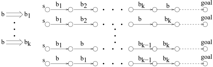
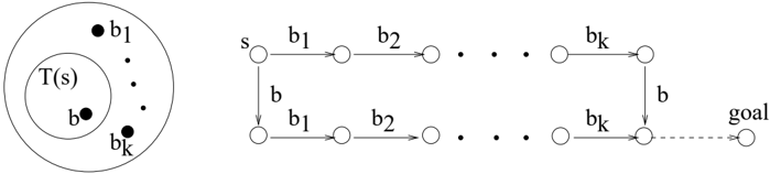
This diagram plots the stubborn set condition A1 in Definition 11.

Fig. 1. Illustration of stubborn set.

Since planning also examines a large search space, we propose to develop a stubborn set theory for planning. To achieve this, we need to handle various subtle issues arising from the differences between model checking and planning. We first define the concept of stubborn sets for planning, adapted from the concepts in model checking.

Definition 11 Stubborn Set for Planning . For a SAS+ planning task, a set of actions T ( s ) is a stubborn set at state s if and only if

• A1) For any action b ∈ T ( s ) and actions b 1 , · · · , b k / ∈ T ( s ) , if ( b 1 , · · · , b k , b ) is a prefix of a path from s to a goal state, then ( b, b 1 , · · · , b k ) is a valid path from s and leads to the same state that ( b 1 , · · · , b k , b ) does; and
• A2) Any valid path from s to a goal state contains at least one action in T ( s ) .

The above definition is schematically illustrated in Figure 1. Once we define the stubborn set T ( s ) at each state s , we in effect reduce the state space graph to a subgraph: only the edges corresponding to actions in the stubborn sets are kept in the subgraph.

Definition 12. For a SAS+ planning task, given a stubborn set T ( s ) defined at each state s , the stubborn set method reduces its state space graph G to a subgraph G r such that V ( G r ) = V ( G ) and there is an edge ( s, s ′ ) in E ( G r ) if and only if there exists an action o ∈ T ( s ) such that s ′ = apply ( s, o ) .

A stubborn set method for planning is a reduction method that reduces the original state space graph G to a subgraph G r according to Definition 12. In other words, a stubborn set method expands actions only in a stubborn set in each state. In the sequel, we show that such a reduction method preserves actions, hence, it also preserves completeness and optimality.

Theorem 1. Any stubborn set method for planning is action-preserving.

Proof. We prove that for any solution sequence ( s 0 , p ) in the original state space graph G , there exists a solution sequence ( s 0 , p ′ ) in the reduced state space graph G r resulting from the stubborn set method, such that p ′ is a permutation of actions in p . We prove this fact by induction on k , the length of p .

When k = 1, let a be the only action in p , according to the second condition in Definition 12, a is in T ( s 0 ). Thus, ( s 0 , p ) is also a solution sequence in G r . The EC method is action-preserving in the base case.

ACM Journal Name, Vol. V, No. N, Month 20YY.

·

When k > 1, the induction assumption is that any path in G with length less than or equal to k -1 has a permutation in G r that leads to the same final state. Now we consider a solution sequence ( s 0 , p ) in G : p = ( a 1 , . . . , a k ). Let s i = apply ( s i -1 , a i ) , i = 1 , . . . , k . If a 1 ∈ T ( s ), we can invoke the induction assumption for the state s 1 and prove our induction assumption for k .

We now consider the case where a 1 / ∈ T ( s ). Let a j be the first action in p such that a j ∈ T ( s ). Such an action must exist because of the condition A2 in Definition 11.

Consider the sequence p ∗ = ( a j , a 1 , · · · , a j -1 , a j +1 , · · · , a k ). According to condition A1 in Definition 12, ( a j , a 1 , · · · , a j -1 ) is also a valid sequence from s 0 which leads to the same state that ( a 1 , · · · , a j ) does. Hence, we know that ( s 0 , p ∗ ) is also a solution path. Therefore, let s ′ = apply ( s 0 , a j ), we know ( a 1 , · · · , a j -1 ) is an executable action sequence starting from s ′ . Let p ∗∗ = ( a 1 , · · · , a j -1 , a j +1 , · · · , a k ), ( s ′ , p ∗∗ ) is a solution sequence in G . From the induction assumption, we know there is a sequence p ′ which is a permutation of p ∗∗ , such that ( s ′ , p ′ ) is a solution sequence in G r . Since a j ∈ T ( s 0 ), we know that a j followed by p ′ is a solution sequence from s 0 and is a permutation of actions in p ∗ , which is a permutation of actions in p . Thus, the stubborn set method is action-preserving. /squaresolid

Since being action-preserving is a sufficient condition for being completenesspreserving and optimality-preserving, when the preference is action set invariant, we have the following result.

Corollary 1. A stubborn set method for planning is completeness-preserving. In addition, it is optimality-preserving when the preference is action set invariant.

3.3 Left commutativity in SAS+ planning

Note that although Theorem 1 provides an important result for reduction, it is not directly applicable since the conditions in Definition 11 are abstract and not directly implementable in algorithms. We need to find sufficient conditions for Definition 11 that can facilitate the design of reduction algorithms. In the following, we define several concepts that can lead to sufficient conditions for Definition 11.

Definition 13 State-Dependent Left Commutativity . For a SAS+ planning task, an ordered action pair ( a, b ) , a, b ∈ O is left commutative in state s , if ( a, b ) is a valid path at s , and ( b, a ) is also a valid path at s and results in the same state. We denote such a relationship by s : b ⇒ a .

Definition 14 State-Independent Left Commutativity . For a SAS+ planning task, an ordered action pair ( a, b ) , a, b ∈ O is left commutative if, for any state s , it is true that s : b ⇒ a . We denote such a relationship by b ⇒ a .

Note the following. 1) Left commutativity is not a symmetric relationship. b ⇒ a does not imply a ⇒ b . 2) The order in the notation b ⇒ a suggests that we should always try only ( b, a ) during the search instead of trying both ( a, b ) and ( b, a ). Also, not every state-independent left commutative action pair is state-dependent left commutative. For instance, in a SAS+ planning task with three state variables { x 1 , x 2 , x 3 } , action a with pre ( a ) = { x 1 = 0 } , eff ( a ) = { x 2 = 1 } and action b with pre ( b ) = { x 2 = 1 , x 3 = 2 } , eff ( b ) = { x 3 = 3 } are left commutative in state

·

In this diagram, the left part plots the condition L1 in Definition 15 and the right part plots the strategy in the proof to Theorem 2.

Fig. 2. Illustration of left commutative set.

s 1 = { x 1 = 0 , x 2 = 1 , x 3 = 3 } but not in state s 2 = { x 1 = 0 , x 2 = 0 , x 3 = 2 } as b is not applicable in state s 2 .

We introduce state-independent left commutativity as it can be used to derive sufficient conditions for finding stubborn sets.

Definition 15 State-Independent Left Commutative Set . For a SAS+ planning task, a set of actions T ( s ) is a left commutative set at a state s if and only if

• L1) For any action b ∈ T ( s ) and any action a ∈ O -T ( s ) , if there exists a valid path from s to a goal state that contains both a and b , then it is the case that b ⇒ a ; and
• A2) Any valid path from s to a goal state contains at least one action in T ( s ) .

Theorem 2. For a SAS+ planning task, for a state s , if a set of actions T ( s ) is a state-independent left commutative set, it is also a stubborn set.

Proof. We only need to prove that L1 in Definition 15 implies A1 in Definition 11. The proof strategy is schematically shown in Figure 2.

For an action b ∈ T ( s ) and actions b 1 , · · · , b k / ∈ T ( s ), if ( b 1 , · · · , b k , b ) is a prefix of a path from s to a goal state, then according to L1, we see that b ⇒ b i , for i = 1 , · · · , k . According to the definition of left commutativity, we see that b k and b can be swapped and that the resulting path ( b 1 , · · · , b, b k ) is still a valid path that leads to the same state that ( b 1 , · · · , b k , b ) does. We can subsequently swap b with b k -1 , · · · , and b 1 to obtain equivalent paths, before finally obtaining ( b, b 1 , · · · , b k ), as shown in the schematic illustration in the right part of Figure 2. Hence, we have shown that if p = ( b 1 , · · · , b k , b ) is a prefix of a path from s to a goal state, then p ′ = ( b, b 1 , · · · , b k ) is a also valid path from s that leads to the same state that p does, which is exactly the condition A 1 in Definition 11. /squaresolid

From the above proof, we see that the requirement of state-independent left commutativity in Definition 15 is unnecessarily strong. Instead, only certain statedependent left commutativity is necessary. In fact, when we change ( b 1 , · · · , b k , b ) to ( b 1 , · · · , b, b k ), we only require s ′ : b ⇒ b k where s ′ is the state after b k -1 is executed. Similarly, when we change ( b 1 , · · · , b k , b ) to ( b 1 , · · · , b, b k -1 , b k ), we only ACM Journal Name, Vol. V, No. N, Month 20YY.

·

require s ′′ : b ⇒ b k -1 where s ′′ is the state after b k -2 is executed. Based on the above analysis, we can refine the sufficient conditions.

Definition 16 State-Dependent Left Commutative Set . For a SAS+ planning task, a set of actions T ( s ) is a left commutative set at a state s if and only if

L1') For any action b ∈ T ( s ) and actions b 1 , · · · , b k / ∈ T ( s ) , if ( b 1 , · · · , b k , b ) is a prefix of a path from s to a goal state, then s ′ : b ⇒ b k , where s ′ is the state after ( b 1 , · · · , b k -1 ) is executed; and

• A2) Any valid path from s to a goal state contains at least one action in T ( s ) .

We only need to slightly modify the proof to Theorem 2 in order to prove the following theorem.

Theorem 3. For a SAS+ planning task, for a state s , if a set of actions T ( s ) is a state-dependent left commutative set, it is also a stubborn set.

The above result gives sufficient conditions for finding stubborn sets in planning. The concept of state-dependent left commutative set requires a less stringent condition than the state-independent left commutative set. Such a nuance actually leads to different previous POR algorithms with varying performances. Therefore, it will result in smaller T ( s ) sets and stronger reduction. Next, we present our algorithm for finding such a set at each state to satisfy these conditions.

3.4 Determining left commutativity

Theorem 3 provides a key result for POR. However, the conditions in Definition 13 are still abstract and not directly implementable. The key issue is to efficiently find left commutative action pairs. Now we give necessary and sufficient conditions for Definition 13 that can practically determine left commutativity and facilitate the design of reduction algorithms.

Theorem 4. For a SAS+ planning task, for a valid action path ( a, b ) in state s , we have s : b ⇒ a if and only if pre ( a ) and eff ( b ) , pre ( b ) and eff ( a ) , eff ( a ) and eff ( b ) are all conflict-free and b is applicable at s .

/negationslash

Proof. First, from the definition of s : b ⇒ a , we know that action b is applicable in state apply ( s, a ). This implies that pre ( b ) and eff ( a ) are conflict-free. Symmetrically, since action a is applicable in state apply ( s, b ), pre ( a ) and eff ( b ) are also conflict-free. Now we prove eff ( a ) and eff ( b ) are conflict-free by contradiction. If eff ( a ) and eff ( b ) are not conflict-free, without loss of generality, we can assume that eff ( a ) contains x i = v i and eff ( b ) contains x i = v ′ i = v i . Thus, the value of x i is v i for state s ab = apply ( apply ( s, a ) , b ) and v ′ i for state s ba = apply ( apply ( s, b ) , a ), i.e., s ab is different than s ba . This contradicts our assumption that a and b are left commutative. Thus, eff ( a ) and eff ( b ) are conflict-free.

Second, if pre ( a ) and eff ( b ), eff ( a ) and pre ( b ), eff ( a ) and eff ( b ) are all conflictfree, since a is applicable in s , a is also applicable in state apply ( s, b ) as pre ( a ) and eff ( b ) are conflict-free. Hence, ( b, a ) is a valid path at s . Also, for any state variable x i , its value in states s ab = apply ( apply ( s, a ) , b ) and s ba = apply ( apply ( s, b ) , a ) are the same, because eff ( a ) and eff ( b ) are conflict-free. Therefore, we have s ab = s ba . Hence, we have s : b ⇒ a . /squaresolid

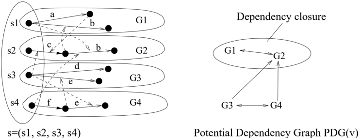
Fig. 3. A SAS+ task with four DTGs. The dashed arrows show preconditions (prevailing and transitional) of each edge (action). Actions are marked with letters a to f. We see that b and e are associated with more than one DTG.

Theorem 4 gives necessary and sufficient conditions for deciding whether two actions are left-commutative or not. Based on this result, we later develop practical POR algorithms that find stubborn sets using left commutativity.

4. EXPLANATION OF PREVIOUS POR ALGORITHMS

Previously, we have proposed two POR algorithms for planning: expansion core (EC) [Chen and Yao 2009] and stratified planning (SP) [Chen et al. 2009], both of which showed good performance in reducing the search space. However we did not have a unified explanation for them. We now explain how these two algorithms can be explained by our theory. Full details of the two algorithms can be found in our papers [Chen and Yao 2009; Chen et al. 2009].

4.1 Explanation of EC

Expansion core (EC) algorithm is a POR-based reduction algorithm for planning. We will see that, in essence, the EC algorithm exploits the SAS+ formalism to find a left commutative set for each state. To describe the EC algorithm, we need the following definitions.

Definition 17. For a SAS+ task, for each DTG G i , i = 1 , . . . , N , for a vertex v ∈ V ( G i ) , an edge e ∈ E ( G i ) is a potential descendant edge of v (denoted as v ✁ e ) if 1) G i is goal-related and there exists a path from v to the goal state in G i that contains e ; or 2) G i is not goal-related and e is reachable from v .

Definition 18. For a SAS+ task, for each DTG G i , i = 1 , . . . , N , for a vertex v ∈ V ( G i ) , a vertex w ∈ V ( G i ) is a potential descendant vertex of v (denoted as v ✁ w ) if 1) G i is goal-related and there exists a path from v to the goal state in G i that contains w ; or 2) G i is not goal-related and w is reachable from v .

/negationslash

Definition 19. For a SAS+ task, given a state s = ( s 1 , · · · , s N ) , for any 1 ≤ i, j ≤ N,i = j , we call s i a potential precondition of the DTG G j if there exist o ∈ O and e j ∈ E ( G j ) such that

ACM Journal Name, Vol. V, No. N, Month 20YY.

/negationslash

·

Definition 20. For a SAS+ task, given a state s = ( s 1 , . . . , s N ) , for any 1 ≤ i, j ≤ N,i = j , we call s i a potential dependent of the DTG G j if there exists o ∈ O , e i = ( s i , s ′ i ) ∈ E ( G i ) and w j ∈ V ( G j ) such that

/negationslash

Definition 21. For a SAS+ task, for a state s = ( s 1 , . . . , s N ) , its potential dependency graph PDG( s ) is a directed graph in which each DTG G i , i = 1 , · · · , N corresponds to a vertex, and there is an edge from G i to G j , i = j , if and only if s i is a potential precondition or potential dependent of G j .

Figure 3 illustrates the above definitions. In PDG( s ), G 1 points to G 2 as s 1 is a potential precondition of G 2 and G 2 points to G 1 as s 2 is a potential dependent of G 1 .

Definition 22. For a directed graph H , a subset C of V ( H ) is a dependency closure if there do not exist v ∈ C and w ∈ V ( H ) -C such that ( v, w ) ∈ E ( H ) .

Intuitively, a DTG in a dependency closure may depend on other DTGs in the closure but not those DTGs outside of the closure. In Figure 3, G 1 and G 2 form a dependency closure of PDG( s ).

The EC algorithm is defined as follows:

Definition 23 Expansion Core Algorithm . For a SAS+ planning task, the EC method reduces its state space graph G to a subgraph G r such that V ( G r ) = V ( G ) and for each vertex (state) s ∈ V ( G ) , it expands actions in the following set T ( s ) ⊆ O :

where exec ( s ) is the set of executable actions in s and C ( s ) ⊆ { 1 , · · · , N } is an index set satisfying:

EC1) The DTGs { G i , i ∈ C ( s ) } form a dependency closure in PDG( s ); and

• EC2) There exists i ∈ C ( s ) such that G i is goal-related and s i is not the goal state in G i .

Intuitively, the EC method can be described as follows. To reduce the original state-space graph, for each state, instead of expanding actions in all the DTGs, it only expands actions in DTGs that belong to a dependency closure of PDG( s ) under the condition that at least one DTG in the dependency closure is goal-related and not at a goal state.

The set C ( s ) can always be found for any non-goal state s since PDG( s ) itself is always such a dependency closure. If there is more than one such closure, theoretically any dependency closure satisfying the above conditions can be used in EC. In practice, when there are multiple such dependency closures, EC picks the one with less actions in order to get stronger reduction. EC has adopted the following scheme to find the dependency closure for any state s .

Given a PDG( s ), EC first finds its strongly connected components (SCCs). If each SCC is contracted to a single vertex, the resulting graph is a directed acyclic

ACM Journal Name, Vol. V, No. N, Month 20YY.

·

graph S . Note that each vertex in S with a zero out-degree corresponds to a dependency closure. It then topologically sorts all the vertices in S to get a sequence of SCCs: S 1 , S 2 , · · · , and picks the minimum m such that S m includes a goal-related DTG that is not in its goal state. It chooses all the DTGs in S 1 , · · · , S m as the dependency closure.

Now we explain the EC algorithm using the POR theory we developed in Section 3. We show that the EC algorithm can be viewed as an algorithm for finding a state-dependent left-commutative set in each state.

Lemma 1. For a SAS+ planning task, the EC algorithm defines a state-dependent left commutative set for each state.

Proof. Consider the set of actions T ( s ) expanded by the EC algorithm in each state s , as defined in (3). We prove that T ( s ) satisfies conditions L1' and A2 in Definition 16.

Consider an action b ∈ T ( s ) and actions b 1 , · · · , b k / ∈ T ( s ) such that ( b 1 , · · · , b k , b ) is a prefix of a path from s to a goal state, we show that s ′ : b ⇒ b k , where s ′ is the state after ( b 1 , · · · , b k -1 ) is applied to s .

Let C ( s ) be the index set of the DTGs that form a dependency closure, as used in in (3). Since b ∈ T ( s ), there must exist m ∈ C ( s ) such that b /turnstileleft G m . Let the state after applying ( b 1 , · · · , b k ) to s be s ∗ . We see that we must have s ∗ m = s m because otherwise there must exist a b j , 1 ≤ j ≤ m that changes the assignment of state variable x m . However, that would imply that b k ∈ T ( s ). Since b is applicable in s ∗ , we see that s m = s ∗ m ∈ pre ( b ).

If there exists a state variable x i such that an assignment to x i is in both eff ( b k ) and pre ( b ), then G m will point to the DTG G i as s m is a potential dependent of G i , forcing G i to be included in the dependency closure, i.e. i ∈ C ( s ). However, as b k /turnstileleft G i , it will violate our assumption that b k / ∈ T ( s ). Hence, none of the precondition assignments of b is added by b k . Therefore, since b is applicable in apply ( s ′ , b k ), it is also applicable in s ′ .

On the other hand, if b k has a precondition assignment in a DTG that b is associated with, then G m will point to that DTG since s m is a potential precondition of b k , forcing that DTG to be in C ( s ), which contradicts the assumption that b k / ∈ T ( s ). Hence, b does not alter any precondition assignment of b k . Therefore, since b k is applicable in s ′ , it is also applicable in the state apply ( s ′ , b ).

Finally, if there exists a state variable x i such that an assignment to x i is altered by both b and b k , then we know b /turnstileleft G i and b k /turnstileleft G i . In this case, G m will point to G i since s m is a potential precondition of G i , making b k ∈ T ( s ), which contradicts our assumption. Hence, eff ( b ) and eff ( b k ) correspond to assignments to distinct sets of state variables. Therefore, applying ( b k , b ) and ( b, b k ) to s ′ will lead to the same state.

From the above, we see that b is applicable in s ′ , b k is applicable in apply ( s ′ , b ), and hence ( b, b k ) is applicable in s ′ . Further we see that ( b, b k ) leads to the same state as ( b k , b ) does when applied to s ′ . We conclude that s ′ : b ⇒ b k and T ( s ) satisfies L1'.

Moreover, for any goal-related DTG G i , if in a state s , its assignment s i is not the goal state in G i , then some actions associated with G i have to be executed in any solution path from s . Since T ( s ) includes all the actions in at least one goal-related

·

DTG G i , any solution path must contain at least one action in T ( s ). Therefore, T ( s ) also satisfies A2 and it is indeed a state-dependent left commutative set. /squaresolid

From Lemma 1 and Theorem 3, we obtain the following result, which shows that EC fits our framework as a stubborn set method for planning.

Theorem 5. For any SAS+ planning task, the EC algorithm defines a stubborn set in each state.

4.2 Explanation of SP

The stratified planning (SP) algorithm exploits commutativity of actions directly [Chen et al. 2009]. To describe the SP algorithm, we need the following definitions first.

/negationslash

Definition 24. Given a SAS+ planning task Π with state variable set X , the causal graph ( CG ) is a directed graph CG (Π) = ( X,E ) with X as the vertex set. There is an edge ( x, x ′ ) ∈ E if and only if x = x ′ and there exists an action o such that x ∈ eff ( o ) and x ′ ∈ pre ( o ) or eff ( o ) .

Definition 25. For a SAS+ task Π , a stratification of the causal graph CG (Π) as ( X,E ) is a partition of the node set X : X = ( X 1 , · · · , X k ) in such a way that there exists no edge e = ( x, y ) where x ∈ X i , y ∈ X j and i > j .

By stratification, each state variable is assigned a level L ( x ), where L ( x ) = i if x ∈ X i , 1 ≤ i ≤ k . Subsequently, each action o is assigned a level L ( o ), 1 ≤ L ( o ) ≤ k . L ( o ) is the level of the state variable(s) in eff ( o ). Note that all state variables in the same eff ( o ) must be in the same level, hence, our L ( o ) is well-defined.

Definition 26 Follow-up Action . For a SAS+ task Π , an action b is a followup action of a (denoted as a /triangleright b ) if eff ( a ) ∩ pre ( b ) = ∅ or eff ( a ) ∩ eff ( b ) = ∅ .

/negationslash

/negationslash

The SP algorithm can be combined with standard search algorithms, such as breadth-first search, depth-first search, and best-first search (including A ∗ ). During the search, for each state s that is going to be expanded, the SP algorithm examines the action a that leads to s . Then, for each applicable action b in state S , SP makes the following decisions.

Definition 27 Stratified Planning Algorithm . For a SAS+ planning task, in any non-initial state s , assuming a is the action that leads directly to s , and b is an applicable action in s , then SP does not expand b if L ( b ) < L ( a ) and b is not a follow-up action of a . Otherwise, SP expands b . In the initial state s 0 , SP expands all applicable actions.

The following result shows the relationship between the SP algorithm and our new POR theory.

Lemma 2. If an action b is not SP-expandable after a , and state s is the state before action a , then s : b ⇒ a .

Proof. Since b is not SP-expandable after a , following the SP algorithm, we have L ( a ) > L ( b ) and b is not a follow-up action of a . According to Definition 26, we have eff ( a ) ∩ pre ( b ) = eff ( a ) ∩ eff ( b ) = ∅ . These imply that eff ( a ) and pre ( b ) are conflict-free, and that eff ( a ) and eff ( b ) are conflict-free. Also, since b is applicable

in apply ( s, a ) and eff ( a ) and pre ( b ) are conflict-free, b must be applicable in s (Otherwise eff ( a ) must change the value of at least one variable in pre ( b ), which means eff ( a ) and pre ( b ) are not conflict-free).

/negationslash

Now we prove that pre ( a ) and eff ( b ) are conflict-free by showing pre ( a ) ∩ eff ( b ) = ∅ . If their intersection is non-empty, we assume a state variable x is assigned by both pre ( a ) and eff ( b ). By the definition of stratification, x is in layer L ( b ). However, since x is assigned by pre ( a ), there must be an edge from layer L ( a ) to layer L ( x ) = L ( b ) since L ( a ) = L ( b ). In this case, we know that L ( a ) < L ( b ) from the definition of stratification. Nevertheless, this contradicts with the assumption that L ( a ) > L ( b ). Thus, pre ( a ) ∩ eff ( b ) = ∅ , and pre ( a ) and eff ( b ) are conflict-free.

With all three conflict-free pairs, we have s : b ⇒ a according to Theorem 2. /squaresolid

Although SP reduces the search space by avoiding the expansion of certain actions, it is in fact not a stubborn set based reduction algorithm. We have the following theorem for the SP algorithm.

Definition 28. For a SAS+ planning task S , a valid path p a = ( a 1 , · · · , a n ) is an SP-path if and only if p a is a path in the search space of the SP algorithm applied to S.

Theorem 6. For a SAS+ planning task S , for any initial s 0 and any valid path p a = ( a 1 , · · · , a n ) from s 0 , there exists a path p b = ( b 1 , · · · , b n ) from s 0 such that p b is an SP-path, and both p a and p b lead to the same state from s 0 , and p b is a permutation of actions in p a .

Proof. We prove by induction on the number of actions.

When n = 1, since there is no action before s 0 , any valid path ( a 1 ) will also be a valid path in the search space of the SP algorithm.

Now we assume this proposition is true of for n = k, k ≥ 1 and prove the case when n = k + 1. For a valid path p 0 = ( a 1 , · · · , a k , a k +1 ), by our induction hypothesis, we can rearrange the first k actions to obtain a path ( a 1 1 , a 1 2 , · · · , a 1 k ).

By the induction hypothesis, if p 1 ′ is still not an SP-path, we can rearrange the first k actions in p 1 ′ to get a new path p 2 = ( a 2 1 , · · · , a 2 k , a 1 k ). Otherwise we let p 2 = p 1 ′ . Comparing p 1 and p 2 , we know L ( a k +1 ) > L ( a 1 k ), namely, the level value of the last action in p 1 is strictly larger than that in p 2 . We can repeat the above process to generate p 3 , · · · , p m , · · · as long as p j ( j ∈ Z + ) is not an SP-path. Our transformation from p j to p j +1 also ensures that every p j is a valid path from s and leads to the same state that p a does.

Now we consider a new path p 1 = ( a 1 1 , · · · , a 1 k , a k +1 ). There are two cases. First, if L ( a k +1 ) < L ( a 1 k ), or L ( a k +1 ) > L ( a 1 k ) and a k +1 is a follow-up action of a 1 k , then p 1 is already an SP-path. Otherwise, we have L ( a k +1 ) > L ( a 1 k ) and a k +1 is not a follow-up action of a 1 k . In this case, by Lemma 2, path p 1 ′ = ( a 1 1 , · · · , a 1 k -1 , a k +1 , a 1 k is also a valid path that leads s to the same state as p a does.

Since we know that the layer value of the last action in each p j is monotonically decreasing as j increases, such a process must stop after a finite number of iterations. Suppose it finally stops at p m = ( a ′ 1 , a ′ 2 , · · · , a ′ k , a ′ k +1 , we must have that L ( a ′ k +1 ) ≤ L ( a ′ k ) or L ( a ′ k +1 ) > L ( a ′ k ) and a ′ k +1 is a follow-up action of a k ′ . Hence, p m now is an SP-path. We then assign p m to p b and the induction step is proved. /squaresolid

·

Theorem 6 shows that the SP algorithm cannot reduce the number of states expanded in the search space. The reason is as follows: for any state in the original search space that is reachable from the initial state s 0 via a path p , there is still an SP-path that reaches s . Therefore, every reachable state in the search space is still reachable by the SP algorithm. In other words, SP reduces the number of generated states, but not the number of expanded states.

SP is not a stubborn set based reduction algorithm. This can be illustrated by the following example.

Assuming a SAS+ planning task S that contains two state variables x 1 and x 2 , where both x 1 and x 2 have domain { 0 , 1 } , with the initial state as { x 1 = 0 , x 2 = 0 } and the goal as { x 1 = 1 , x 2 = 1 } . Actions a and b are two actions in S where pre ( a ) is { x 1 = 0 } and eff ( a ) is { x 1 = 1 } and pre ( b ) is { x 2 = 0 } and eff ( b ) is { x 2 = 1 } . It is easy to see that a and b are not follow-up actions of each other, and that x 1 , x 2 will be in different layers after stratification. Without loss of generality, we can assume L ( a ) = L ( x 1 ) > L ( x 2 ) = L ( b ). Therefore, we know that action b will not be expanded after action a in state s : { x 1 = 1 , x 2 = 0 } . However, apply ( s, b ) is the goal. Not expanding b in state s violates condition A 2 in Definition 11 where any valid path from s to a goal state has to contain at least one action in the expansion set of s .

We can also see in the above example that the search space explored by SP contains four states, namely, the initial state s 0 , apply ( s 0 , a ), apply ( s 0 , b ) and the goal state. Meanwhile, under the EC algorithm, in state s 0 , the DTGs for x 1 and x 2 are not in each other's dependency closures. This implies that in s 0 , EC expands either action a or b , but not both. Therefore, EC expands three states while SP expands four. This illustrates our conclusion in Theorem 6 that the SP algorithm cannot reduce the number of expanded states.

5. A NEW POR ALGORITHM FRAMEWORK FOR PLANNING

We have developed a POR theory for planning and explained two previous POR algorithms using the theory. Now, based on the theory, we propose a new POR algorithm which is stronger than the previous EC algorithm.

Our theory shows in Theorem 3 that the condition for enabling POR reduction is strongly related to left commutativity of actions. In fact, constructing a stubborn set can be reduced to finding a left commutativity set. As we show in Theorem 5, the EC algorithm follows this idea. However, the basic unit of reduction in EC is DTG (i.e. either all actions in a DTG are expanded or none of them are), which is not necessary according to our theory. Based on this insight, we propose a new algorithm that operates with the granularity of actions instead of DTGs.

Definition 29. For a state s , an action set L is a landmark action set if and only if any valid path starting from s to a goal state contains at least one action in L .

Definition 30. For a SAS+ task, an action a ∈ O is supported by an action b if and only if pre ( a ) ∩ eff ( b ) = ∅ .

/negationslash

Definition 31. For a state s , its action support graph (ASG) at s is defined as a directed graph in which each vertex is an action, and there is an edge from a

ACM Journal Name, Vol. V, No. N, Month 20YY.

to b if and only if a is not applicable in s and a is supported by b .

The above definition of ASG is a direct extension of the definition of a causal graph. Instead of having domains as basic units, here we directly use actions as basic units.

Definition 32. For an action a and a state s , the action core of a at s , denoted by AC s ( a ) , is the set of actions that are in the transitive closure of a in ASG ( s ) . The action core for a given set of actions A is the union of action cores of every action in A .

/negationslash

Lemma 3. For a state s , if an action a is not applicable in s and there is a valid path p starting from s whose last action is a , then p contains an action b, b = a, b ∈ AC s ( a ) .

Proof. We prove this by induction on the length of p .

In the base case where | p | = 2, we assume p = ( b, a ). Since a is not applicable in s , it must be supported by b . Thus, b ∈ AC s ( a ). Suppose this lemma is true for 2 ≤ | p | ≤ k -1, we prove the case for | p | = k . For a valid path p = ( o 1 , . . . , o k ), again there exists an action b before a that supports a . If b is applicable in s , then b ∈ AC s ( a ). Otherwise, we have a path p ′ = ( o 1 , . . . , b ) with 2 ≤ | p ′ | ≤ k -1. Thus, by the induction assumption, p ′ contains at least one action in AC s ( b ), which is a subset of AC s ( a ), according to Definition 31 and 32. /squaresolid

Definition 33. Given a SAS+ planning task Π with O as set of all actions O , for a state s and a set of action A , the action closure of action set A at s , denoted by by C s ( A ) , is a subset of O and a super set of A such that for any applicable action a ∈ C s ( A ) at s and any action b ∈ O \ C s ( A ) , eff ( a ) and eff ( b ) are conflict-free. In addition, if pre ( b ) ∈ S , eff ( a ) and pre ( b ) are conflict-free.

Intuitively, actions in C s ( A ) can be executed without affecting the completeness and optimality of search. Specifically, because any applicable action in C s ( A ) and any action not in C s ( A ) will not assign different values to the same state variable, for action a ∈ C s ( A ) and action b ∈ O \ C s ( A ) at s , path ( a, b ) will lead to the same state that ( b, a ) does. Additionally, because pre ( b ) and eff ( a ) are conflict-free when pre ( b ) ∈ s , executing action a will not affect the applicability of action b in future. Therefore, actions in C s ( A ) can be safely expanded first during the search, while actions outside it can be expanded later.

A simple procedure, shown in Algorithm 1, can be used to find the action closure for a given action set A .

The proposed POR algorithm, called stubborn action core (SAC), works as follows. At any given state s , the expansion set E ( s ) of state s is determined by Algorithm 2.

There are various ways to find a landmark action set for a given state. Here we give one example that is used in our current implementation. To find a landmark action set L at s , we utilize the DTGs associated with the SAS+ formalism. We first find a transition set that includes all possible transitions ( s i , v i ) in an unachieved goal-related DTG G i where s i is the current state of G i in s . It is easy to see that all actions that mark transitions in this set make up a landmark action set, because

ACM Journal Name, Vol. V, No. N, Month 20YY.

·

input : A SAS+ task with action set O , an action set A ⊆ Q , and a state s output : An action closure C ( A ) of A

/negationslash

C ( A ) ← A ; repeat foreach action a in C ( A ) applicable in s do foreach action b in O \ C ( A ) do if pre ( b ) ∩ s = ∅ and pre ( b ) and eff ( a ) are not conflict-free then C ( A ) ← C ( A ) ∪ { b } ; end if eff ( b ) and eff ( a ) are not conflict-free then C ( A ) ← C ( A ) ∪ { b } ; end end end until C ( A ) is not changing ; return C ( A ) ; Algorithm 1: A procedure to find action closure input : A SAS+ planning task and state s output : The expansion set E ( s ) Find a landmark action set L at s ; Calculate the action core AC s ( L ) of L using Algorithm 1; Use AC s ( L ) as E ( s ) ;

Algorithm 2: The SAC algorithm

G i is unachieved and at least one action starting from s i has to be performed in any solution plan.

There are also other ways to find a landmark action set. For instance, the preprocessor in the LAMA planner [Richter et al. 2008] can be used to find landmark facts, and all actions that lead to these landmark facts also make up a landmark action set.

Theorem 7. For a state s , the expansion set E ( s ) defined by the SAC algorithm is a stubborn set at s .

Proof. We first prove that our expansion set E ( s ) satisfies condition A 1 in Definition 11, namely, for any action b ∈ E ( S ), and actions b 1 , · · · , b k / ∈ E ( s ), if ( b 1 , · · · , b k , b ) is a valid path from s , then ( b, b 1 , · · · , b k ) is also a valid path, and leads to the same state that ( b 1 , · · · , b k , b ) does.

To simplify this proof, we can treat action sequence ( b 1 , · · · , b k ) as a 'macro' action B where an assignment x t = v t in pre ( B ) if and only if x t = v t is in the precondition of some b i ∈ B and x t = v t is not in the effects of a previous action b j ( j < i ), and an assignment x t = v t is in eff ( B ) if and only if x t = v t is in the effect set of some b i ∈ B , and x t is not assigned to any value other than v t in the effects of later action b j ( j > i ). In the following proof, we use the macro action B in place of the path ( b 1 , · · · , b k ).

To prove A 1, we only need to prove that if ( B,b ) is a valid path, then s : b ⇒ B . According to Theorem 4, s : b ⇒ B if and only if the following four propositions are true.

a) Action b must be applicable in s . We prove this by contradiction. Let s ′ = apply ( s, B ), if b is not applicable in s , but applicable in s ′ , then B supports b . Since all effects of B are from actions in the path ( b 1 , · · · , b k ), there exists an action b i ∈ { b 1 , · · · , b k } such that b i supports b . However, according to Definition 32, b i is in the transitive closure of b in ASG ( s ). According to our algorithm, b i should be in E ( s ). This contradicts with our assumption that b i / ∈ E ( s ). Thus, b must be applicable at s .

b) pre ( B ) and eff ( b ) are conflict-free. We prove this proposition by contradiction. If pre ( B ) and eff ( b ) are not conflict-free, we assume that pre ( B ) has x t = v t that conflicts with an assignment in eff ( b ). According to the way we define B , there exists an action b i ∈ ( b 1 , · · · , b k ), such that x t = v t . Also, since B is applicable in s , we know that x t takes the value v t at s also. Therefore, we know that pre ( b i ) and eff ( b ) are not conflict-free. However, according to Definition 33 and Algorithm 1, b i is in E ( s ). This contradicts with our assumption that b i is not in E ( s ). Thus, pre ( B ) and eff ( b ) are conflict-free.

c) eff ( B ) and eff ( b ) are conflict-free. The proof of this proposition is very similar to the one above. If they are not conflict-free, we must have action b i ∈ ( b 1 , · · · , b k ), such that eff ( b ) and eff ( b i ) are not conflict-free. However, according to Definition 33 and Algorithm 1, b i is in E ( s ). This contradicts with our assumption that b i is not in E ( s ). Thus, eff ( B ) and eff ( b ) are conflict-free.

d) pre ( b ) and eff ( B ) are conflict-free. This proposition is true as we assumed in condition A 1 that ( B,b ) is a valid path from s .

Thus, from Theorem 4, we see that s : b ⇒ B and that condition A 1 in Definition 11 is true.

Now we verify condition A 2 by showing that any solution path p from s contains at least one action in E ( s ). From the definition of landmark action sets, we know that there exists an action l ∈ L such that p contains l . From Lemma 3 we know that AC s ( l ) contains at least one action, applicable in s , in p . Thus, E ( s ) indeed contains at least one action in p .

Since E ( s ) satisfies conditions A 1 and A 2 in Definition 11, E ( s ) is a stubborn set in state s .

/squaresolid

5.1 SAC vs. EC

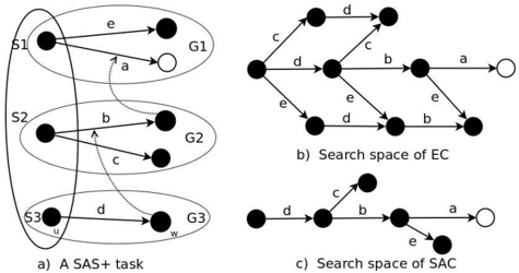
SAC gives stronger reduction than the previous EC algorithm, since it is based on actions, which have a finer granularity than DTGs do. Specifically, SAC gives more reduction than EC for two reasons. First, applicable actions that are not associated with landmark transitions, even if they are in the same DTG, are expanded by EC but not by SAC. Second, applicable actions that do not support any actions in the landmark action set, even if they are in the same DTG, are expanded by EC but not by SAC.

To give an example, in Figure 4a, G1, G2, G3 are three DTGs. The goal assignment is marked as an unfilled circle in G1. a, b, c, d, e are actions. Dashed arrows denote the preconditions of actions. For instance, the lower dashed arrow means

ACM Journal Name, Vol. V, No. N, Month 20YY.

that b requires a precondition x 3 = w .

In this example, according to EC, G1 is a goal DTG and G2 and G3 are in the dependency closure of G1. Thus, before executing a , EC expands every applicable action in G1, G2 and G3 at any state. SAC, on the other hand, starts with a singleton set { a } as the initial landmark action set and ignores action e . Applicable action c is also not included in the action closure in state s since it does not support a . The search graphs are compared in Figure 4 and we see that SAC gives stronger reduction.

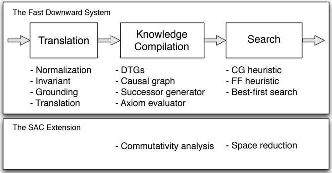
6. SYSTEM IMPLEMENTATION

We adopt the Fast Downward (FD) planning system [Helmert 2006] as our code base. The overall architecture of FD is described in Figure 5. A complete FD system contains three parts corresponding to three phases in execution: translation, knowledge compilation and search. Translation module will convert planning tasks

ACM Journal Name, Vol. V, No. N, Month 20YY.

·

described into a SAS+ planning task. The knowledge compilation module will generate domain transition graphs and causal graph for the SAS+ planning task. The search module implements various state-space-search algorithms as well as heuristic functions. All these three modules communicate by temporary files.

We make two additions to the above system to implement our SAC planning system, as shown in Figure 5. First, we add a 'commutativity analysis' module into the knowledge compilation step to identify commutativity between actions. Second, we add a 'space reduction' module to the search module to conduct state space reduction. The commutativity analysis module is used to build left commutativity relations between actions and build the action support graph. It reads action information from the output of knowledge compilation module and determines the left commutativity relations between actions according to conditions in Theorem 3. In addition, this module also determines if one action is supported by another and builds the action support graph defined in Definition 31. The reduction module for search is used to generate a stubborn set of a given state. We implement the SAC algorithm in this module. Starting from a landmark action set L as the target action set, we find the action closure AC s ( L ) iteratively add actions that support actions in the target action set to the target action set until it is not changing. We then use the applicable actions in the action closure as the set of actions to expand at s . In other words, in our SAC system, during the search, for any given state s , instead of using successor generator provided by FD to generate a set of applicable operators, we use the reduction module to generate a stubborn set in state s and use it as the expansion set.

It is easy to see that the overall time complexity of determining left commutativity relationships between actions is O ( | A | 2 ) where | A | is the number of actions. We implement this module in Python. Since the number of actions | A | is usually not large, in most of the cases, the commutativity analysis module takes less than 1 second to finish. This module only runs once for solving a planning problem. Therefore, the commutativity analysis module amounts to an insignificant amount of overhead to the system. Theoretically, the worst case time complexity for finding the action closure is O ( | A | 2 ) where | A | is the number of actions. However, in practice, by choosing the landmark action set L that associated with transitions in an unarchived goal-related DTG starting from current state, the procedure of finding action closure terminates quickly after about 4 to 5 iterations. Therefore, adding the reduction module does not increase the overall search overhead significantly either. We implement this module in C++ and incorporate it into the search module of FD.

7. EXPERIMENTAL RESULTS

We test our algorithm on problems in the recent International Planning Competitions (IPCs): IPC4, and IPC5. We implemented our algorithm on top of the Fast Downward (FD) planner [Helmert 2006]. We only modified the state expansion part.

We have implemented our SAC algorithm and tested it along with Fast Downward and its combination with the EC extension on a Red Hat Linux server with 2Gb memory and one 2.0GHz CPU. The admissible HSP h max heuristic [Bonet and

ACM Journal Name, Vol. V, No. N, Month 20YY.

·

Geffner 2001] and inadmissible Fast Forward (FF) heuristic [Hoffmann and Nebel 2001] are used in our experiments.

First, we apply our SAC algorithm to A ∗ search with the HSP h max heuristic [Bonet and Geffner 2001]. We also turn off the option of preferred operators [Helmert 2006] since it compromises the optimality of A ∗ search. Table I shows the detailed results on node expansion and generation during the search. We also compare the solving times of these three algorithms. As we can clearly see from Table I, the numbers of expanded nodes of the SAC-enhanced A ∗ algorithm are consistently lower than those of the baseline A ∗ algorithm and the EC-enhanced A ∗ algorithm. There are some cases where the generated nodes of the SAC-enhanced algorithm are slightly larger than those of the baseline A ∗ or EC-enhanced A ∗ algorithm. This is possible due to the tie-breaking of states with equal heuristic values during search.

We can also see that the computational overhead of SAC is low. For instance, in the Freecell domain, the running time of the SAC-enhanced algorithm is only slightly higher than the baseline and lower than the EC-enhanced algorithm, despite their equal number of expanded and generated nodes.

Aside from the A ∗ algorithm, we also test SAC on best-first search algorithms. Although POR preserves completeness and optimality, it can also be combined with suboptimal searches such as best-first search to reduce their search space. In this comparison, we turned off the option of preferred operators in our experiment for FD. Preferred operator is another space reduction method that does not preserve completeness, and using it with EC or SAC will lead to worse performance. We will investigate how to find synergy between these two approaches in our future work. We summarize the performance of three algorithms, original Fast Downward (FD), FD with EC, and FD with SAC, in Table II by presenting the number of problem instances in a planning domain that can be solved within 1800 seconds by each solver. We also ignore small problem instances with solving time less than 0 . 01 seconds. All there solvers uses inadmissible Fast Forward (FF) heuristic. As we can see from Table II, when combined with a best-first-search algorithm, SAC can still reduce the number of generated and expanded nodes compared to the baseline FD algorithm and the EC-enhanced algorithm. In many problems (e.g. pipesworld18 , tpp15 , truck13 ), the saving on the number of expanded states can be of orders of magnitude.

8. RELATED WORK

We discuss some related work in this section.

8.1 Symmetry

Symmetry detection is another way for reducing the search space [Fox and Long 1999]. From the view of node expansion on a SAS+ formalism for planning, we can see that symmetry removal is different from SAC. For example, consider a domain with three objects A 1 , A 2 , and B , where A 1 and A 2 are symmetric, and actions associated with B have no conflict with any actions associated with A 1 or A 2 . In this case, symmetry removal will expand actions associated with ( A 1 and B ) or ( A 2 and B ), whereas SAC will only expand actions associated with the DTG for B if we pick a landmark action set based on it. This is because both the action

core and the action closure will not include any actions associated with A 1 or A 2 as they have no conflict with actions in B .

Intuitively, symmetric removal finds that it is not important whether A 1 or A 2 is used since they are symmetric, whereas SAC finds that it is not important whether actions associated with B is used before or after actions associated with A i , i = 1 , 2 since there is no conflict. In fact, SAC can also detect stronger relationships such as the fact that it is safe to use actions associated with B before those associated with A i , since any path that uses actions associated with A i before those associated with B corresponds to another valid path with the same cost.

Further, there is limited research on domain-independent detection and removal of symmetry. The method by Fox and Long [Fox and Long 1999] detects symmetry from the specification of initial and goal states and may miss many symmetries.

8.2 Factored planning

Factored planning [Amir and Engelhardt 2003; Brafman and Domshlak 2006; Kelareva et al. 2007] is a class of search algorithms that exploits the decomposition of state space. In essence, factored planning finds all the subplans for each individual subgraph and tries to merge them. There are some limitations of factored planning.

First, for some problems with dense subgraphs, the number of subplans in each subgraph may be very large, making the search very expensive. What is worse is that there are many subgraphs in which the goal is not specified, leading to more subplans that need to be considered. We have done some empirical study on this matter. For example, for pipesworld20, there are 96 DTGs, 18 out of which have goal facts. Even if we only consider one DTG and apply the canonicality assumption that each state can be included at most once in any subplan, the number of subplans from the initial state to the goal can be as high as 1.96 × 10 9 in DTG #16 generated by Fast Downward. The number is high because there are multiple transition paths, and each transition can be associated with many actions. If we multiply the numbers of possible subplans of the 18 DTGs containing goals, the number will approximately be of the order of 10 120 . Thus, the search space will be extremely large if we consider all the 96 DTGs (78 of which do not even have a goal state) and remove the canonicality assumption. Of course, techniques such as tree search and pruning [Kelareva et al. 2007] can speed up the process but the potential speedup is largely unknown.

Second, since the canonicality assumption is generally not true for many domains, and there are potentially infinite number of subplans without restriction on the subplan length, the factored planning algorithm needs to use certain schemes such as iterative deepening [Brafman and Domshlak 2006] to restrict the subplan length. These schemes further increase the complexity and may compromise the global optimality of the resulting plan [Kelareva et al. 2007].

In summary, although factored planning has shown potential on some domaindependent studies, its practicality for general domain-independent planning has not been established yet. We note that POR algorithms we studied in this paper are not exclusive to factored planning and it is possible that POR can be integrated into factored planning to reduce the cost of search.

8.3 Planning utilizing the SAS+ decomposition

Our POR method is based on the SAS+ representation [Helmert 2006]. Recently there has been increasing interest in utilizing the SAS+ representation.

The Fast Downward planner [Helmert 2006] develops its heuristic function by analyzing the causal graphs on top of the SAS+ models. Another SAS+ based heuristic for optimal planning is recently obtained via a linear programming model encoding DTGs [van den Briel et al. 2007]. The LAMA planner derives inadmissible heuristic values by analyzing landmarks in SAS+ models [Richter et al. 2008]. An admissible version of it is proposed in [Karpas and Domshlak 2009] by using action cost partitioning. Yet another admissible heuristic called 'mergeand-shrink' is developed based on abstraction of domain transitions [Helmert et al. 2007], which strictly dominates the admissible landmark heuristics [Helmert and Domshlak 2009]. Moreover, long-distance mutual exclusion constraints based on a DTG analysis is proposed and shown to be effective in speeding up SAT-based optimal planners [Chen et al. 2009]. The DTG-Plan planner searches directly on the space of DTGs in a hierarchical decomposition fashion [Chen et al. 2008]. The algorithm is shown to be fast but is not complete or optimal.

Comparing to the above recent work, POR offers a completely new approach to exploit the state-space decomposition in the SAS+ representation. It is orthogonal to the design of better heuristics and it provides a systematical, theoretically sound way to reduce search costs.

POR is most effective for problems where the action support graphs are directional and the inter-action dependencies are not dense. It may not be useful for problems where the actions are strongly connected and there is a high degree of inter-action dependencies. For example, it is not useful for the 15-puzzle where each action on each piece is supported by surrounding actions, which makes the action support graph strongly connected. In this case, POR cannot give reductions during the search.

9. CONCLUSIONS AND FUTURE WORK

Previous work in both model checking and AI planning has demonstrated that POR is a powerful method for reducing search costs. POR is an enabling technique for modeling checking, which will not be practical without POR due to its high complexity. Although POR has been extensively studied for model checking, its theory has not been developed for AI planning. In this paper, we developed a new POR theory for planning that is parallel to the stubborn set theory in model checking.

In addition, by analyzing the structure of actions in planning problems, we derived a practical criterion that defines left commutativity between actions. Based on the notion of left commutativity, we developed sufficient conditions for finding stubborn sets during search for planning.

Furthermore, we applied our theory to explain two previous POR algorithms for planning. The explanation provided useful insights that lead to a stronger and more efficient POR algorithm called SAC. Compared to previous POR algorithms, SAC finds stubborn sets based on a finer granularity for checking left commutativity, leading to strong reduction. We compared the performance of SAC to the previously

·

·

proposed EC algorithm on both optimal and non-optimal state space searches. Experimental results showed that the proposed SAC algorithm led to significantly stronger node reduction and less overhead.

In our future work, we plan to develop stronger POR algorithms for planning based on our theoretical framework and study its interaction with other search reduction techniques such as preferred operators [Helmert 2006], abstraction heuristics [Helmert et al. 2007], landmarks [Richter et al. 2008], and symmetry detection [Fox and Long 1999].

REFERENCES

• Amir, E. and Engelhardt, B. 2003. Factored planning. In Proc. IJCAI .
• Bonet, B. and Geffner, H. 2001. Planning as heuristic search. Artificial Intelligence, Special issue on Heuristic Search 129, 1.
• Brafman, R. and Domshlak, C. 2006. Factored planning: How, when, and when not. In Proc. AAAI .
• Briel, M. V. D. , Benton, J. , and Kambhampati, S. 2007. An lp-based heuristic for optimal planning. In 13th International Conference on Principles and Practice of Constraint Programming . 651-665.
• Chen, Y. , Huang, R. , and Zhang, W. 2008. Fast planning by search in domain transition graphs. In Proc. AAAI .
• Chen, Y. , Xu, Y. , and Yao, G. 2009. Stratified planning. In Proc. IJCAI .
• Chen, Y. and Yao, G. 2009. Completeness and optimality preserving reduction for planning. In Proc. IJCAI .
• Chen, Y. , Zhao, X. , and Zhang, W. 2009. Long distance mutual exclusion for planning. Artificial Intelligence 173, 2, 365-391.
• Clarke, E. M. , Grumberg, O. , and Peled, D. A. 2000. Model Checking . The MIT Press.
• Fox, M. and Long, D. 1999. The detection and exploitation of symmetry in planning problems. In Proc. IJCAI .
• Helmert, M. 2006. The Fast Downward planning system. Journal of Artificial Intelligence Research 26 , 191-246.
• Helmert, M. and Domshlak, C. 2009. Landmarks, critical paths and abstractions: What's the difference anyway? In Proc. ICAPS .
• Helmert, M. , Haslum, P. , and Hoffmann, J. 2007. Flexible abstraction heuristics for optimal sequential planning. In Proc. ICAPS . 176-183.
• Helmert, M. and R¨ oger, G. 2008. How good is almost perfect. In Proc. AAAI .
• Hoffmann, J. and Nebel, B. 2001. The FF planning system: Fast plan generation through heuristic search. Journal of Artificial Intelligence Research 14 , 253-302.
• Holzmann, G. J. 1997. The model checker spin. IEEE Trans. on Software Engineering 23 , 279-295.
• Jonsson, P. and B¨ ackstr¨ om, C. 1998. State-variable planning under structural restrictions: Algorithms and complexity. Artificial Intelligence 100, 1-2, 125-176.
• Karpas, E. and Domshlak, C. 2009. Cost-optimal planning with landmarks. In Proceedings of the 21st international jont conference on Artifical intelligence . Morgan Kaufmann Publishers Inc., 1728-1733.
• Kelareva, E. , Buffet, O. , Huang, J. , and Thi´ ebaux, S. 2007. Factored planning using decomposition trees. In Proc. IJCAI .
• Richter, S. , Helmert, M. , and Westphal, M. 2008. Landmarks revisited. In Proceedings of the Twenty-Third AAAI Conference on Artificial Intelligence . AAAI Press.
• Valmari, A. 1988. State space generation: Efficiency and practicality. Ph.D. thesis, Tampere University of Technology Publications.
• Valmari, A. 1989. Stubborn sets for reduced state space generation. In Proceedings of the 10th International Conference on Applications and Theory of Petri Nets .

ACM Journal Name, Vol. V, No. N, Month 20YY.

• Valmari, A. 1990. A stubborn attack on state explosion. In Proceedings of the 1990 International Workshop on Computer Aided Verification .
• Valmari, A. 1991. Stubborn sets of coloured petri nets. In Proceedings of the 12th International Conference on Application and Theory of Petri Nets . 102-121.
• Valmari, A. 1993. On-the-fly verification with stubborn sets. In CAV '93: Proceedings of the 5th International Conference on Computer Aided Verification . Springer-Verlag, London, UK, 397-408.
• Valmari, A. 1998. The state explosion problem. Lectures on Petri Nets I: Basic Models, Lecture Notes in Computer Science 1491 , 429-528.
• van den Briel, M. , Benson, J. , Kambhampati, S. , and Vossen, T. 2007. An LP-based heuristic for optimal planning. In Proc. Constraint Programming Conference .
• Varpaaniemi, K. 2005. On stubborn sets in the verification of linear time temporal properties. Formal Methods in System Design 26, 1, 45-67.

Table I: Comparison of FD, EC, and SAC using A* with h max heuristic on IPC domains. We show numbers of expanded and generated nodes. '-' means timeout after 300 seconds. For each problem, we also highlight the best values of expanded and generated nodes among three algorithms, if there is any difference.

Domain	FD			EC			SAC
	Expanded	Generated	Time	Expanded	Generated	Time	Expanded	Generated	Time
airport 1	9	9	0	9	9	0	9	9	0
airport 2	16	17	0	16	17	0	16	17	0
airport 3	38	102	0	35	90	0.01	✄ ✂ /a0 ✁ 27	✄ ✂ /a0 ✁ 43	0.01
airport 4	21	21	0	21	21	0.01	21	✄ ✂ /a0 ✁ 20	0.01
airport 5	22	28	0	22	28	0.01	22	✄ ✂ /a0 23	0.01
airport 6	138	335	0.01	120	230	0.07	✄ /a0 86	✁ ✄ /a0 202	0.06
airport 7	221987	5305641	81.02	221987	5305641	91.07	✂ ✁ ✄ ✂ /a0 ✁ 221901	✂ ✁ ✄ ✂ /a0 ✁ 709575 /a0	74.95
airport 8	2420	11190	0.73	2364	6621	1.93	✄ ✂ /a0 ✁ 699	✄ ✂ 2860	0.56
airport 9	11005	60058	4.66	11005	39027	16.35	✄ ✂ /a0 ✁ 4923	✁ ✄ ✂ /a0 ✁ 24244	5.86
airport 10	19	20	0.01	19	20	0.01	19	✄ /a0 ✁ 18	0.01
airport 11	22	28	0.01	22	28	0.01	22	✂ ✄ /a0 23	0.01
airport 12	122	328	0.03	104	119	0.07	✄ ✂ /a0 ✁ 80	✂ ✁ ✄ ✂ /a0 ✁ 195	0.06
airport 13	112	295	0.01	94	182	0.07	✄ ✂ /a0 76	✄ ✂ /a0 187	0.08
airport 14	2300	11144	0.84	2246	6324	2.14	✁ ✄ ✂ /a0 ✁ 626	✁ ✄ ✂ /a0 ✁ 2700	0.61
airport 15	1910	9240	0.69	1904	5396	1.94	✄ ✂ /a0 ✁ 493	✄ ✂ /a0 ✁ 2124	0.46
depot 1	159	1000	0.01	159	1000	0.02	159	✄ /a0 981	0.02
depot 2	2294	17803	0.01	2310	17894	0.52	2294	✂ ✁ ✄ /a0 ✁ 16404	0.34
depot 3	2389	21172	0.2	2389	✄ /a0 ✁ 20724	0.3	2389	✂ 21168	0.76
depot 4	42435	366989	5.08	42435	✂ 366989	7.08	✄ /a0 ✁ 42362	✄ /a0 ✁ 364883	4.35
depot 5	13096	119388	2.35	13096	119388	4.15	✂ 13096	✂ 119388	3.07

continued on next page

·

continued from previous page

Domain	FD			EC			SAC
	Expanded	Generated	Time	Expanded	Generated	Time	Expanded /a0	Generated	Time
depot 7	9672	91795	0.81	9672	91795	1.89	✄ ✂ ✁ 9658	✄ ✂ /a0 ✁ 91460 ✄	1.73
depot 8	173184	1999709	40.15	173184	1999709	60.8	✄ ✂ /a0 ✁ 173157	✂ /a0 ✁ 1993740	51.68
drivelog 1	57	373	0	57	355	0	✄ /a0 30	✄ /a0 183	0
drivelog 2	55780	417679	2.35	55387	393334	3.2	✂ ✁ ✄ ✂ /a0 ✁ 52124	✂ ✁ ✄ ✂ /a0 ✁ 325004 /a0	4.12
drivelog 3	2982	22693	0.12	2858	21247	0.16	✄ ✂ /a0 ✁ 2682	✄ ✂ ✁ 19774	0.13
drivelog 4	460727	4798803	31.33	446341	4175538	35.38	✄ ✂ /a0 ✁ 414148	✄ ✂ /a0 4004775	28.65
drivelog 5	2077987	24224013	167.86	2040088	✄ ✂ /a0 22120590	202.42	✄ ✂ /a0 ✁ 1943657	✁ 22156584	168.73
freecell 1	63	407	0.01	63	✁ 407	0.01	63	407	0.03
freecell 2	212	1603	0.06	212	1603	0.18	212	1603	0.23
freecell 3	162	1156	0.07	162	1156	0.37	162	1156	0.26
freecell 4	792	4765	0.35	792	4765	2.35	792	4765	1.76
freecell 5	526	2930	0.49	526	2930	1.81	526	2930	1.81
freecell 6	430	2834	0.88	430	2834	3.39	430	2834	2.38
freecell 7	1429	8347	2.5	1429	8347	5.5	1429	8347	4.02
freecell 8	1682	12015	6.68	1682	12015	16.21	1682	12015	14.66
freecell 9	2001	12122	7.44	2001	12122	18.42	2001	12122	16.32
freecell 10	1953	14383	11.66	1953	14383	31.57	1953	14383 /a0	23.54
rover 1	323	2043	0	323	2043	0.01	✄ ✂ /a0 ✁ 114 /a0	✄ ✂ 558	0
rover 2	161	1019	0	161	1019	0	✄ ✂ ✁ 64	✁ ✄ ✂ /a0 239	0
rover 3	863	5724	0.01	863	5724	0.04	✄ ✂ /a0 ✁ 390	✁ ✄ ✂ /a0 ✁ 2007	0.01
rover 4	291	2399	0	291	2399	0.01	✄ /a0 79	✄ ✂ /a0 397	0
rover 5	324204	5714884	6.42	324204	5714884	9.23	✂ ✁ ✄ ✂ /a0 ✁ 95369	✁ ✄ ✂ /a0 ✁ 1093514	5.1
rover 6	-	-	-	-	-	-	✄ ✂ /a0 ✁ 251276	✄ ✂ /a0 ✁ 2437578 /a0	10.48
rover 7	156150	2179859	2.64	156150	2179859	5.21	✄ ✂ /a0 ✁ 34772	✄ ✂ ✁ 387527	2.01

continued on next page

·

continued from previous page

Domain	FD			EC			SAC
	Expanded	Generated	Time	Expanded	Generated	Time	Expanded	Generated ✄ /a0	Time
truck 1	390	4306	0.03	390	4306	0.03	390 ✄ /a0	✂ ✁ 1145 ✄ /a0	0.04
truck 2	943	13212	0.01	943	13212	0.12	✂ ✁ 942 ✄ /a0	✂ ✁ 2432 ✄ /a0	0.11
truck 3	9162	178481	1.12	9162	178481	1.82	✂ ✁ 9157 ✄ /a0	✂ ✁ 44098 ✄ /a0	1.03
truck 4	37799	258286	1.77	8792	15177	1.77	✂ ✁ 6841	✂ ✁ 12570	1.51

Table II: Comparison of FD, EC and SAC with no-preferred operators on IPC's domains. Weshow numbers of expanded and generated nodes. '-' means timeout after 1800 seconds. For each problem, we also highlight the best values of expanded and generated nodes among three algorithms if there is any difference.

Domains	FD			EC			SAC
	Expanded	Generated	Time	Expanded	Generated	Time	Expanded	Generated	Time
airport 13	✄ /a0 ✁ 43	106	0.03	46	102	0.08	45	✄ /a0 ✁ 68 /a0	0.05
airport 14	✂ 78	321	0.07	70	199	0.19	70	✂ ✄ ✂ 161	0.12
airport 15	67	224	0.06	66	163	0.2	✄ ✂ /a0 ✁ 64	✁ ✄ ✂ /a0 141	0.12
airport 16	310	1541	0.35	315	1549	1.05	310	✁ ✄ ✂ /a0 740	0.62
airport 17	815	4682	1.15	21819	140496	101.16	✄ ✂ /a0 809	✁ ✄ ✂ /a0 2315	2.1
airport 18	✄ ✂ /a0 ✁ 18653	142281	44.3	82007	655661	529.57	✁ 18712	✁ ✄ ✂ /a0 ✁ 76214	78.78
airport 19	10564	65299	15.07	10621	65480	48.12	✄ ✂ /a0 ✁ 5041	✄ ✂ /a0 17123	15.5
airport 20	✄ ✂ /a0 ✁ 25377	182487	52.94	150816	1272996	959.32	25636	✁ ✄ ✂ /a0 ✁ 116148	53.58
airport 21	102	274	0.24	102	256	1.57	102	✄ ✂ /a0 ✁ 193 /a0	0.56
airport 22	149	524	0.51	150	509	3.34	149	✄ ✂ ✁ 370	1.52
airport 23	169	620	0.81	169	561	6.03	169	✄ ✂ /a0 ✁ 500	1.51
airport 24	166	888	1.14	1902	7459	70.58	✄ ✂ /a0 ✁ 111	604	1.08
airport 25	33751	197109	256.95	-	-	-	✄ ✂ /a0 ✁ 18752	✄ ✂ /a0 ✁ 66186	161.84
driveslog 11	24	284	0.01	24	284	0.02	87	949	0.05
driveslog 12	78	1059	0.05	✄ ✂ /a0 ✁ 64	✄ /a0 ✁ 224	0.04	150	1875	0.13
driveslog 13	583	6396	0.25	75	✂ 864	0.06	75	864	0.07
driveslog 14	248	3378	0.13	75	883	0.07	75	✄ ✂ /a0 416	0.05
driveslog 16	64971	1331293	146.32	50855	1017221	110.91	✄ ✂ /a0 ✁ 38746	✁ ✄ ✂ /a0 ✁ 737836 /a0	142.11
driveslog 17	24860	804116	204.9	149938	5012829	1253.07	✄ ✂ /a0 ✁ 15620	✄ ✂ ✁ 537050	138.37
driveslog 19	834	26406	9.77	727	14443	7.37	✄ ✂ /a0 ✁ 573	✄ ✂ /a0 ✁ 1105	5.19

continued on next page

·

continued from previous page

Domains	FD			EC			SAC
	Expanded	Generated	Time	Expanded	Generated	Time	Expanded	Generated	Time
freecell 1	10	59	0.08	11	63	0.09	10	✄ ✂ /a0 ✁ 54	0.08
freecell 2	17	114	0.1	17	114	0.1	17	✄ ✂ /a0 ✁ 100	0.01
freecell 3	20	144	0.3	✄ ✂ /a0 ✁ 19	✄ ✂ /a0 ✁ 122	0.14	20	127	0.13
freecell 4	48	268	0.39	61	401	0.26	✄ ✂ /a0 ✁ 35	✄ ✂ /a0 ✁ 238	0.17
freecell 5	88	510	0.62	123	668	0.82	✄ ✂ /a0 ✁ 63	✄ ✂ /a0 ✁ 236 /a0	0.35
freecell 6	98	510	0.74	97	496	0.71	✄ ✂ /a0 ✁ 58 ✄	✄ ✂ 384 ✄	0.7
freecell 7	412	1594	4.26	233	884	1.93	✂ /a0 ✁ 215	✁ ✂ /a0 ✁ 814	2.23
freecell 8	106	700	1.02	✄ ✂ /a0 ✁ 71	✄ ✂ /a0 ✁ 436	0.83	85	501	1.13
freecell 9	✄ ✂ /a0 ✁ 68	✄ ✂ /a0 ✁ 500	2.6	112	667	3.93	122	719	3.3
freecell 10	797	5043	50.79	4057	34183	217.53	✄ ✂ /a0 ✁ 112	✄ ✂ /a0 ✁ 597 /a0	5.49
freecell 11	120	530	3.72	119	620	4.07	✄ ✂ /a0 ✁ 118	✄ ✂ ✁ 527	4.21
freecell 12	192	1085	5.6	✄ ✂ /a0 ✁ 58	✄ ✂ /a0 ✁ 420	2.58	96	491	3.51
freecell 13	✄ ✂ /a0 ✁ 412	✄ ✂ /a0 ✁ 2655	10.21	589	2896	9.26	592	2996	13.16
freecell 14	287	2274	31.27	339	2054	29.96	✄ ✂ /a0 ✁ 78	✄ ✂ /a0 560	8.86
freecell 15	1913	8642	140.72	531	2795	35.44	✄ ✂ /a0 ✁ 248	✁ ✄ ✂ /a0 1197	18.21
freecell 16	3818	31173	143.88	409	2381	10.87	✄ ✂ /a0 ✁ 371	✁ ✄ ✂ /a0 ✁ 1722 /a0	7.14
freecell 17	246	1402	19.71	244	2849	23.62	✄ ✂ /a0 ✁ 104	✄ ✂ 740	10.99
freecell 18	3480	✄ ✂ /a0 ✁ 17263	354.43	6069	32509	685.41	✄ ✂ /a0 ✁ 3036	✁ 19476	174.69
pipesworld 7	13	685	1.19	13	685	0.73	13	685	0.71
pipesworld 8	12	550	0.79	12	✄ ✂ /a0 ✁ 473	0.74	12	531	0.79
pipesworld 9	319	8297	10.05	✄ ✂ /a0 ✁ 165	5002	6.31	166	✄ ✂ /a0 ✁ 4996	5.74
pipesworld 10	✄ ✂ /a0 ✁ 50	✄ ✂ /a0 ✁ 1572 /a0	2.92	115	3322	5.14	168	4684	7.4
pipesworld 11	✄ ✂ /a0 ✁ 197	✄ ✂ ✁ 970	0.34	451302	2168501	459.77	1615	7311	4.24

continued on next page

·

continued from previous page

Domains	FD			EC			SAC
	Expanded	Generated	Time	Expanded	Generated	Time	Expanded ✄ /a0	Generated /a0	Time
pipesworld 13	-	-	-	8083	54502	40.44	✂ ✁ 4272	✄ ✂ ✁ 20342	6.16
pipesworld 14	3412	16652	6.01	✄ ✂ /a0 2520	✄ ✂ /a0 11302	4.33	2815	13066	10.66
pipesworld 15	568191	2792188	1284.82	✁ 561869	✁ 2776786	1405.04	✄ ✂ /a0 ✁ 93320	✄ ✂ /a0 802500 ✄	316.24
pipesworld 17	156733	561923	292.99	✄ ✂ /a0 ✁ 89829	334833	188.93	93169	✁ ✂ /a0 ✁ 324196	140.06
pipesworld 18	21164	230257	1049.83	491	5057	30.25	491	✄ ✂ /a0 ✁ 2948 ✄ /a0	28.16
pipesworld 20	-	-	-	-	-	-	✄ ✂ /a0 ✁ 1417 ✄ /a0	✂ ✁ 30469 ✄ /a0	596.39
pipesworld 21	4486	29504	32.43	-	-	-	✂ ✁ 896	✂ ✁ 4412	8.38
tpp 8	675	4987	0.12	✄ ✂ /a0 ✁ 570	✄ ✂ /a0 ✁ 3854	0.14	581	4735	0.16
tpp 9	✄ ✂ /a0 ✁ 570	✄ ✂ /a0 ✁ 3839	0.09	960	7430	0.28	1184 ✄ /a0	10098 ✄ /a0	0.29
tpp 10	585	5861	0.13	3679	37791	1.18	✂ ✁ 442 ✄	✂ ✁ 4186 ✄	0.14
tpp 11	6294	68216	3.21	3815	33688	1.93	✂ /a0 ✁ 2678 ✄ /a0	✂ /a0 ✁ 28276 ✄ /a0	1.75
tpp 12	12922	139267	7.42	6888	63805	3.88	✂ ✁ 1947 ✄ /a0	✂ ✁ 22579 ✄ /a0	1.56
tpp 13	7757	91630	6.8	5554	70013	5.49	✂ ✁ 4555 ✄ /a0	✂ ✁ 58212 ✄ /a0	4.68
tpp 14	12291	1705578	190.82	15700	211138	22.96	✂ ✁ 6054 ✄	✂ 76611 ✄	8.02
tpp 15	9203	112319	15.12	13788	181676	29.22	✂ /a0 ✁ 3149	✁ ✂ /a0 36960	4.82
tpp 16	-	-	-	48549	783502	176.84	✄ ✂ /a0 ✁ 17808 ✄	✁ ✄ ✂ /a0 256920 ✄	61.04
tpp 20	-	-	-	-	-	-	✂ /a0 ✁ 278126	✁ ✂ /a0 ✁ 4503504	1309.18
storage 13	✄ ✂ /a0 ✁ 1353	✄ ✂ /a0 ✁ 4606	0.18	1354	4607	0.25	1634 ✄	5645	0.68
storage 14	265	2727	0.2	212	2137	0.19	✂ /a0 ✁ 172 /a0	✄ ✂ /a0 ✁ 1829	0.26
storage 15	57	✄ ✂ /a0 ✁ 603	0.13	59	622	0.13	✄ ✂ ✁ 56 ✄ /a0	629 ✄ /a0	0.18
storage 16	52	697	0.25	31	412	0.21	✂ ✁ 26	✂ 357	0.22
storage 17	✄ ✂ /a0 ✁ 308	✄ ✂ /a0 ✁ 4128	0.63	337	4480	0.77	339 ✄	✁ 4553 ✄	1.15
storage 18	361	5628	1.68	482	6173	1.86	✂ /a0 ✁ 346	✂ /a0 ✁ 5402	2.42

continued on next page

·

continued from previous page

Domains	FD			EC			SAC
	Expanded /a0	Generated	Time	Expanded	Generated	Time	Expanded	Generated	Time
storage 19	✄ ✂ ✁ 133171	✄ ✂ /a0 ✁ 1426180	594.48	133771	1442383	607.67	133425	1436330	619.37
truck 1	22	230	0.01	22	230	0.01	22	✄ ✂ /a0 ✁ 74	0.01
truck 2	327	4434	0.05	327	4434	0.07	✄ ✂ /a0 ✁ 113	✄ ✂ /a0 ✁ 298	0.03
truck 3	35	672	0.05	35	672	0.05	✄ ✂ /a0 ✁ 34	✄ ✂ /a0 ✁ 148 /a0	0.05
truck 4	40	931	0.02	40	931	0.03	40	✄ ✂ ✁ 227	0.02
truck 5	37	1255	0.05	37	1255	0.05	✄ ✂ /a0 ✁ 35 /a0	✄ ✂ /a0 244	0.05
truck 6	47	1822	0.08	47	1822	0.09	✄ ✂ 41	✁ ✄ ✂ /a0 255	0.07
truck 7	23913	525066	9.24	23913	525066	9.76	✁ 23914 /a0	✁ ✄ ✂ /a0 ✁ 80585 /a0	8.32
truck 8	300	9217	0.24	300	9217	0.23	✄ ✁ 257	✄ 798	0.17
truck 9	3390	154042	2.87	3390	154042	2.95	✂ 3390	✂ ✁ 154042 ✄	2.95
truck 10	139416	8111005	179.09	139416	8111005	186.29	✄ ✂ /a0 ✁ 86993 ✄ /a0	✂ /a0 ✁ 218926 ✄ /a0	46.46
truck 11	4715	344079	13.89	4715	344079	14.25	✂ 4526	✂ 12044	8.38
truck 12	320765	30119993	1357.29	320765	30119993	1352.82	✁ 320790 ✄	✁ ✄ ✂ /a0 ✁ 1068035 /a0	518.89
truck 13	525967	27598625	1181.73	525967	27598625	1182.49	✂ /a0 ✁ 289825 /a0	✄ ✂ ✁ 698071	349.43
truck 14	37380	863543	46.23	37380	863543	47.36	✄ ✂ ✁ 20713	✄ ✂ /a0 ✁ 496998 /a0	36.68
truck 15	59659	1356218	79.9	59659	1356218	84.26	✄ ✂ /a0 ✁ 57584	✄ ✂ ✁ 148886	62.78
truck 17	-	-	-	-	-	-	✄ ✂ /a0 ✁ 159519 /a0	✄ ✂ /a0 ✁ 452932 /a0	553.03
rover 7	30	464	0.01	30	464	0.01	✄ ✂ 20	✄ ✂ 224	0.01
rover 8	36	866	0.01	36	866	0.02	✁ ✄ ✂ /a0 28	✁ ✄ ✂ /a0 554	0.01
rover 9	281	5865	0.06	368	8349	0.11	✁ ✄ ✂ /a0 ✁ 113 /a0	✁ ✄ ✂ /a0 ✁ 1148	0.02
rover 10	232	7321	0.09	232	7321	0.12	✄ ✂ ✁ 81	✄ ✂ /a0 ✁ 1186 /a0	0.03
rover 11	1074	24425	0.28	1074	24425	0.35	✄ ✂ /a0 ✁ 418	✄ ✂ ✁ 7754 /a0	0.13
rover 12	26	531	0.01	26	531	0.01	26	✄ ✂ ✁ 438	0.01

continued on next page

·

continued from previous page

Domains	FD			EC			SAC
	Expanded	Generated	Time	Expanded	Generated	Time	Expanded	Generated /a0	Time
rover 13	175	4523	0.09	175	4523	0.12	191	✄ ✂ ✁ 3685	0.1
rover 14	81	2075	0.03	81	2075	0.04	215	2424 /a0	0.06
rover 15	570	16587	0.25	570	16587	0.29	✄ ✂ /a0 ✁ 499 ✄	✄ ✂ ✁ 15850 ✄ /a0	0.17
rover 16	545	13945	0.24	545	13945	0.27	✂ /a0 ✁ 103 ✄ /a0	✂ ✁ 1771 ✄ /a0	0.05
rover 17	-	-	-	445	16811	0.54	✂ 172 ✄	✂ 2319	0.11
rover 18	37590	1532969	52.87	37590	1532969	63.4	✁ ✂ /a0 ✁ 4801	✁ ✄ ✂ /a0 ✁ 110878 /a0	4.77
openstack 5	39	171	0.01	39	171	0.01	39	✄ ✂ ✁ 170	0.01
openstack 6	109	712	0.05	109	712	0.06	109	712 ✄ /a0	0.08
openstack 7	100	673	0.05	100	673	0.06	100 ✄ /a0	✂ ✁ 672 ✄ /a0	0.09
pathway 3	28	344	0.01	28	344	0.01	✂ ✁ 22 ✄ /a0	✂ ✁ 84 /a0	0.01
pathway 4	76	726	0.01	76	726	0.03	✂ ✁ 61 ✄ /a0	✄ ✂ 624 /a0	0.01
pathway 5	47	1296	0.02	47	1296	0.03	✂ 37 ✄	✁ ✄ ✂ ✁ 1061 ✄ /a0	0.02
pathway 6	255	6402	0.12	255	6402	0.28	✁ ✂ /a0 ✁ 68	✂ 626	0.04
pathway 7	21147 ✄	750778	20.76	21147	750778	47.21	21147	✁ ✄ ✂ /a0 ✁ 533384 ✄ /a0	17.28
pathway 8	✂ /a0 ✁ 21507	858174	24.93	-	-	-	39088 ✄ /a0	✂ ✁ 472722 ✄ /a0	31.25
pathway 9	-	-	-	471	13639	1.39	✂ ✁ 151	✂ ✁ 2155	0.19

·