Topological Parameters for time-space tradeoff

Rina Dechter

Information and Computer Science University of California, Irvine dechter@ics. uci. edu

Abstract

In this paper we propose a family of algo­ rithms combining tree-clustering with condi­ tioning that trade space for time. Such algo­ rithms are useful for reasoning in probabilis­ tic and deterministic networks as well as for accomplishing optimization tasks. By ana­ lyzing the problem structure it will be possi­ ble to select from a spectrum the algorithm that best meets a given time-space specifica­ tion.

1 INTRODUCTION

while reasonable time complexity guarantees are main­ tained. Is it possible to have the time guarantees of clustering while using linear space? On some problem instances, it is possible. Specifically, on those problems whose associated graph has a tree width and a cutset of comparable sizes (e.g., on a ring, the cutset size is 1 and the tree width is 2, leading to identical time bounds). In general, however, it is probably not pos­ sible, because in general the minimal cycle-cutset of a graph can be much larger than its tree width, namely, r $ c + 1, where cis the minimal cycle-cutset and r is the tree width. Furthermore, we conjecture that any algorithm that has a time bound that is exponential in the tree-width will, on some problem instances, require exponential space in the tree width.

Topology-based algorithms for constraint satisfac­ tion and probabilistic reasoning fall into two distinct classes. One class is centered on tree-clustering, the other on cycle-cutset decomposition. Tree-clustering involves transforming the original problem into a tree­ like problem that can then be solved by a specialized tree-solvin g. algorithm [Mackworth and Freuder, 1985; Pearl, 1986j. The tree-clustering algorithm is time and space exponential in the induced width (also called tree width) of the problem's graph. The transforming algo­ rithm identifies subproblems that together form a tree, and the solutions to the subproblems serve as the new values of variables in a tree metalevel problem. The metalevel problem is called a join-tree.

The cycle-cutset method exploits the problem's struc­ ture in a different way. A cycle-cutset is a subset of the nodes in a graph which cuts all of the graph's cy­ cles. A typical cycle-cutset method enumerates the possible assignments to a set of cutset variables and, for each cutset assignment, solves (or reasons about) a tree-like problem in polynomial time. The overall time complexity is exponential in the size of the cycle­ cutset [Dechter, 1992]. Fortunately, enumerating all the cutset's assignments can be accomplished in linear space.

Since the space complexity of tree-clustering can severely limit its usefulness, we investigate the ex­ tent to which its space complexity can be reduced,

The space complexity of tree-clustering can be bounded more tightly using the separator width, which is defined as the size of the maximum subset of vari­ ables shared by adjacent subproblems in the join-tree. Our initial investigation employs separator width to control the time-space tradeoff. The idea is to com­ bine adjacent subproblems joined by a large separator into one big cluster so that the remaining separators are of smaller size. Once a join-tree with smaller sep­ arators is generated, its potentially larger clusters can be solved using the cycle-cutset method.

We will develop such time-space tradeoffs for belief network processing, constraint processing, and opti­ mization tasks, yielding a sequence of algorithms that can trade space for time. With this characterization it will be possible to select from a spectrum of algorithms the one that best meets some time-space requirement. Algorithm tree-clustering and cycle-cutset decomposi­ tion are two extremes in this spectrum.

We introduce the ideas using belief networks (section 2) and then show how they are applicable to con­ straint networks (section 3) and to optimization prob­ lems (section 4).

2 PROBABILISTIC NETWORKS

The observation that methods based on condition­ ing are inferior time-wise and superior space-wise in

a worst-case sense to methods based on clustering is not widely acknowledged in belief network processing. T h is can be partially attributed to [ S hac ht e r et a/., 1 991], wh e r e it is argued that conditioning is a special case of clustering. While there are always abstract cri­ t e ri a according to which one algorithm can be viewed a special case of another, one should not abstract away the hard fact that conditioning takes linear space while clustering is space hungry.

A belief n et w o r k is a concise description of a com­ p le te probability distribution. It is d e fi ne d by a di­ rected acyclic graph over nodes representing random variables, and each variable is annotated with the con­ ditional probability matrices specifying its probability given each value combination of its parent variables. A belief network uses the concept of a directed graph.

Definition 1 [Directed g r a p h ] A directed graph G = { V , E }, where V = { X 1, ... ,Xn} is a set of elements and E::::: {(X;,Xj)IX;,Xi E V} is the set of edges. If an arc (X;, Xi) E E, we s a y that X; points to Xi. Fo r each variable X;, pa( X;) is the set of variables pointing to X; in G, w hil e ch(X;) is the set of va r iabl es that X; p o i n t s to. The family of X, includes X, and its parent variables. A directed graph is acyclic if it has no directed cycles.

Definition 2[Belief Netwo rk s ] Let X= {X1, ... ,Xn} be a s e t of random variables over multi-valued do­ mains, D1, ... , Dn. A belief network is a pair (G, P) where G is a directed acyclic graph and P = {Pi} are the conditional probability matrices over the fam­ i l ie s of G, P; = {P(Xdpa(X;)}. An as si g n m e n t (X1 = Xt, . .. , Xn = xn) can be abbreviated as x = ( x 1, ... , xn). The belief network re p re s e n t s a probability distribu­ tion over X having the product form

wh ere Xpa(X;) d e n o t es the projection of a tuple x ov er pa(Xi)· An evidence set e is an instantiated subset of variables. A moral graph of a belief network is an undi­ re c t e d graph generated by connecting any two head­ to-head pointing arcs in the belief n e t wo r k ' s directed graph and removing t h e a r r ows .

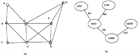
F ig u r e 1 shows a belief network's acyclic graph and its associated moral graph. Two of the m o st common tasks over b e l i e f networks are determining posterior beliefs and, given a set of observations finding the most probable explanation (MPE).

2.1 TREE-CLUSTERING

The most widely used method for processing belief net­ works is tree-clustering. Tree-clustering methods have two parts: determining the structure of the newly gen­ erated tree problem, and assembling the conditional probabilistic distributions between subproblems. The structure of the join-tree is generated using graph in­ formation only. F i rs t the m o r a l graph is embedded in a chordal graph by adding some edges. This is normally accomplished by picking a variable ordering d = X1, · . · , Xn, then, moving from X,. to X1, recur­ sively connecting all the neighbors of X; that precede it in the o rder i ng . The induced width (or tree wi d th ) of this o r d e r e d gr aph , d en o t e d w *(d), is the maximal number of earlier n e i gh b o rs in the resulting graph of each node. The maximal cliques in the newly gener­ ated chordal graph form a clique-tree and serve as the subproblems (or clusters) in the final tree, the join­ tree. The i n duc ed w id th w * (d) equals the maximal clique minus 1. The size of the smallest induced width o ve r all the graph's clique-tree embeddings is th e in­ duced width (or, tree-width), W* of the graph. A subset of nodes is called a cycle-cutset if t h e i r removal makes the graph cycle-free.

Once the tree structure is d e t e r m i n e d , each subprob­ l e m is viewd as a metavariable whose values are all the value combinations of the original variables in the clus­ ter. The conditional probabilities between neighboring cliques c an then be computed [Pearl, 1988]. A l t e r na ­ tively, the marginal p r o b a bi l i t y distributions for each clique can be computed [Lauritzen and Spi eg elh a lte r , 1988]. In b o t h cases, the c o mput a t i o n is e xpone nt ial in the clique's size, so clustering is time and space ex­ p o n e n t ia l in the moral graph's induced-width [Pearl, 1988; Lauritzen and Spiegelhalter, 1988}.

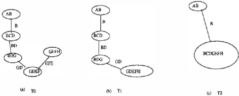
Example 1: Since the moral graph in Figure 1 (b) is c h o rda l no arc is added in the first step of clus­ tering. The maximal cliques of t h e chordal graph are {(A, B), (B, C, D), (B, D, G), (G, D, E, F), (H, G, F, E )}, a n d an associated join-tree is given in Figure 2(a). The tree width of this problem is 3, the separator width is 3, and its minimal cycle-cutset has size 3 ( G , D, E is a c y cl e -c ut s et ) . A b rut ef or c e application of tree­ clustering to this problem is time an d space exponen­ tial in 4.

The implementation of tree-clustering can be tailored to particular queries, to yield better space complexity on some insta n c es. For instance, one way to c o m p u te the belief of a particular variable, once the structure of a join-tree is available, is to generate a rooted join­ tree whose root-clique contains the variable whose be­ lief we wish to update. Then cliques can be processed recursively from leaves to the root. Processing a clique involves computing the marginals over the separators,

which is defined as the intersection between the clique and its parent clique. A brute-force way of accom­ plishing this is to multiply the probabilistic functions in the clique for each clique's tuple and accumulate a sum over the variables in the clique that do not par­ ticipate in the separator. Such computation is time exponential in the clique's size, but it requires only linear space to record the oputput. In our case, the output space is exponential in the separator's size (See example in section 2.4).

Once the computation of a clique terminates, the com­ puted marginal on its separator is added to the parent clique and the clique is removed. Computation re­ sumes over new leaf-cliques until only the root-clique, containing the variable whose belief we wish to assess, remains1. Such a modification is applicable to vari­ ous tasks and, in particular, to belief assessment and MPE.

This modification tightens the bound on space com­ plexity by using the separator width of the join-tree. The separator width of a join-tree is the maximal size of the intersections between any two cliques, and the separator width of a graph is the minimal separator width among the separator widths over all the graph's clique-tree embeddings.

In summary,

Theorem 1: [time-space of clustering] Gwen a be­ lief network whose moral graph can be embedded in a clique-tree having induced width r and separator width s, the time complexity for determining the beliefs and the MPE is O(n · exp(r)) while the space complexity is O(n · exp(s)). 0

Clearly s � r. Note that since in our example the sep­ arator width is 3 and the tree width is also 3, we do not gain much space-wise by the modified algorithm out­ lined above. There are, however, many cases where the separator width is much smaller than the tree width.

2.2 CUTSET CONDITIONING

Alternatively, belief networks may be processed by cutset conditioning [Pearl, 1988]. Conditioning com­ putes conditioned beliefs and MPE for each assign­ ment to a cycle-cutset, using a tree algorithms ap­ plied to the tree resulting from deleting the condition­ ing variables, and then computes the overall belief by taking a weighted sum or performing a maximization. The weights are the belief associated with each cut­ set assignment. The time complexity of conditioning is therefore worst-case exponential in the cycle-cutset size of the network's moral graph and it is space linear. This latter fact is not obvious since it requires comput­ ing the beliefs of every cutset's value combination, in linear time and space.

1 We disregard algorithmic details that do not affect asymptotic worst-ca.5e analysis here.

Lemma 1: Given a moral graph and given a cycle­ cutset C, computing the belief of C = c is time and space linear.

2.3 TRADING SPACE FOR TIME

Assume now that we have a problem whose join-tree has induced width r and separator width s but space restrictions do not allow the necessary O(exp(s)) mem­ ory required by (modified) tree-clustering. One way to overcome this problem is to collapse cliques joined by large separators into one big cluster. The result­ ing join-tree has larger subproblems but smaller sep­ arators. This yields a sequence of tree-decomposition algorithms parameterized by the sizes of their separa­ tors.

Definition 3[Primary and secondary join-trees]: Let T be a clique-tree embedding of the moral graph G. Let s0, s1 , ... , Sn be the sizes of the separators in T listed in strictly descending order. With each separa­ tor size s;, we associate a tree decomposition T; gener­ ated by combining adjacent clusters whose separator sizes are strictly greater than s;. T = To is called the primary join-tree, while n. when i > 0, is a secondary join-tree. We denote by r; the largest cluster size in T; minus 1.

Note that as s; decreases, r; increases. Clearly, from Theorem 1, it follows that

Theorem 2: Given a join-tree T, belief updating and MPE computation can be accomplished using any one of the following time and space bounds b;, where b; = (O(n·exp(ri)) time, and O(n·exp(s;)) space). 0

We know that finding the smallest tree width of a graph is NP-hard [Arnborg, 1985; Arnborg et a/., 1987]; nevertheless, many greedy ordering algorithms provide useful upper bounds that can be inspected in linear time. We denote by W*· the smallest tree width among all the tree embeddings of G whose separators are of sizes or less. Finding W*· may be hard as well, however. We conclude:

Corollary 1: Given a belief network B N, for any s � n, belief updating and MPE can be computed in time O(exp(w*,)), ifO(exp(s)) space can be used. 0

Finally, instead of executing a brute-force algorithm to compute the marginal joint probability distributions over the cliques, we can use the conditioning scheme and then record the marginals over the separators only. This leads to the following conclusion:

Theorem 3: Given a constant s ::::; n, belief assess­ ment and M P E determination can be done in space O(n · e:�:p(s)) and in time O(n · e:�:p(c·,)), where C*· is the maximum size of a minimal cycle-cutset in any subnetwork defined by a cluster in a cli q ue-tree whose separator width is of size s or less, while assuming S::::; C*·. 0

Example 2: When Theorem 2 is applied to the belief network in Figure 1 using the join-trees given in Fig­ ure 2, we see that finding the beliefs and an MPE can be accomplished in either O(k4) time and O(k3) space (based on the primary join-tree T0), or O(k5) time and O(k2) space (based on TI), or O(e) time and linear space (based on T2). In these cases, the joint distribu­ tions over the s u bp r ob le m s defined by the c l i q u e s were presumably computed by a brute-force algorithm. If we apply cutset conditioning to each such subnetwork, we get no improvement in the bound for To because the largest cutset size in a cluster is 2. For T1, we can im­ prove the time bound from O(k5) to O(k4) with only 0( exp(2)) space (because the cutset size of the sub­ graph restricted to {G,D,E,F,H}, is 2); and when applying conditioning to the clusters in T2, we get a time bound of O(k5) with just linear space (because here, using T 2 the cycle-cutset of the whole problem is 3). Thus, the dominating tradeoffs (when considering only the exponents) are between an algorithm based on T1 that requires O(k4) time and quadratic space and an algorithm based on T 2 that requires O(k5) time and linear space.

shrink The special case of singleton separators was dis­ cussed previously in the context of belief networks. When the moral graph can be decomposed to nonsep­ arable components, the conditioning method can be modified to be time exponential in the maximal cut­ set in each c om r o n e n t only [Peot and Shachter, 1991; Darwiche, 1995 .

2.4 EXAMPLE

We conclude this section by demonstrating in details the mechanics of processing a subnetwork by tree­ clustering, by a brute-force methods and by condi­ tioning applied to our example in Figure 1. We will use the join-tree T -2 and process cluster { B, C, D, E, F, G, H}. Processing this cluster amounts to computing the marginal distribution over the sepa­ rator B, namely (we annotate constant by primes):

Migrating the components as far to the left as possi­ ble to exploit a variable elimination scheme which is similar to clustering (for details see [Dechter, 1996]), we get:

Clustering. Summing on the variables one by one from right to left, while recording intermediate tables is equivalent to tree-clustering. First, summing over h yields the function hn(g,/, e)= Lh P(h/g,/, e). This takes time exponential in 4 (since there are 4 vari­ ables) and space exponential in 3 to record the 3-arity resulting function. Subsequently, summing over F we compute hp(g,e,d) = L.. 1 P(J/g)P(eld,J)hn(g,f,e), which is also time exponential in 4 and space expo­ nential in 3. Summing over C yields, hc(g, e, d, b') = L.. P(c/b')P(djc)hF(g, e, d) in time exponential in 4 ( re�ember that b' is fixed) and in space exponential in 3. Continuing in this way we compute he(g, d, b') = Le h c (g, e, d, b') (which is time exponential in 3 and space exponential in 2), then, summing over G, re­ sults in ha(d, b') = L g P(glb', d)hE(g, d) (time expo­ nential in 2 and space exponential in 1) and, finally, P(b') = Ld hc(d, b'}. Overall, the computation per each variable is time exponential in 4 and space expo­ nential in 3.

Brute-force. Alternatively we can do the same com­ putation in a brute-force manner. The same initial ex­ pression along the same variable ordering can be used. In this case we expand the probability tree in a forward manner assigning values one by one (conditioning) to all variables, and computing the tuple's probability. We can save computation by using partial common paths of the tree. With this approach we can compute P(b) in time exponential in 6 (the size of the probabil­ ity tree) and using linear space, since the sums can be accumulated while traversing the tree in a depth-first manner.

Conditioning. A third option is to use consi­ tioning within the cluster. Assume we condition on D, G, E. This makes the resulting problem a tree. Mechanically, it means that we will expand the probability tree forward using variables D, G, E, and for every assighnment g, d, e w e will use vari­ able elimination (or clustering) in a backwards man­ ner, while treating d, g, e as constant. We per­ form the backwards computation (denoting constants by primes) as follows. We compute hn (g', f, e') = LhP(hjg',f,e'). This takes time exponential in 2 and space exponential in 1. Subsequently, com­ pute hp(g', e', d') = L j P(f/g')P(e'/d', J)Hh(g', f, e') which takes time exponential in 1 and constant space. Finally, sum the result over variable C: hc(u',e',d',b') = EcP(c/b')P(d'jc)Hp(g',e',d') in time exponential in 1 and constant space. So far we

spent time exponential in 2 and space exponential in 1 at the most. Since we have to repeat this for every value of g, d, e the overall time will be eponential in 5 while the space will be linear.

3 CONSTRAINT NETWORKS

Definition 4 [Constraint network]: A constraint network consists of a finite set of variables X {Xl, . . . , X n } , each associated with a domain of discrete values, D1, ... , D n and a set of con­ straints, { C1, ... , Ct}. A constraint is a relation, de­ fined on some subset of variables, whose tuples are all the compatible value assignments. A constraint C; has two parts: (1) the subset of variables S; :::: {X;,, ... , X;j(>)}, on which the constraint is defined, called a constraint subset, and (2) a relation, rei;, de ­ fined over S; : rei; � D;, x · · · x D;,<;> . The scheme of a constraint network is the set of subsets on which constraints are defined. An assignment of a unique domain value to each member of some subset of vari­ ables is called an instantiation. A consistent instanti­ ation of all the variables is called a solution. Typical queries associated with constraint networks are to de­ termine whether a solution exists and to find one or all solutions.

Definition 5[Constraint graphs]: Two graphical rep­ resentations of a constraint network are its primal con­ straint graph and its dual constraint graph. A pnmal constraint graph represents variables by nodes and as­ sociates an arc with any two nodes residing in the same constraint. A dual constraint graph represents each c on str a i n t subset by a node and associates a labeled arc with any two nodes whose constraint subsets share variables. The arcs are labeled by the shared variables.

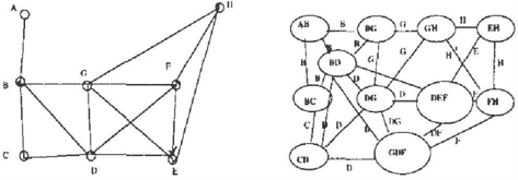
Example 3: Figure 3 depicts the primal and the dual representations of a network having variables A, B, C, D, E, F, G, H whose constraints are de­ fined on the subsets {(A, B), (B, C), (B, D), (C, D), (D, G), (G, E), (B, G), (D,�, JC), (G, D, JC), (G,H), (�, H)(JC, H)}.

Tree-clustering for constraint networks is very similar to tree-clustering for probabilistic networks. In fact, the structuring part is identical. First, the constraint graph is embedded in a clique-tree, then the solution set for each clique is computed. This latter compu­ tation is exponential in the clique's size. Therefore, clustering has time and space complexities that are ex­ ponential in the induced width of its constraint graph [Pearl, 1988; Lauritzen and Spiegelhalter, 1988].

Example 4: Since the graph in Figure 3(a) is iden­ tical to the graph in Figure 1 (b), it possesses the same clique-tree em beddings. Namely, the maximal cliques of the chordal graph are {(A, B), (B, C, D), (B, D, G), (G, D, �.F), (H, G, F, E)} and the join-tree is g i v e n in Figure 2(a). The schemes of the subproblems associ­ ated with each clique are: CAB :::: {(A, B)}, CBcD :::: {(B, C), (C, D)}, CBDG = {(B, D), (B, G), (G, D)}, CcvEF {(G, D)(D, E), (E, F)(G, F)(D, F)} CcEFH :::: {(E, F)(G, F)(G, H)(F, H)(E, H)}. As in the probabilistic case, a brute-force application of tree­ clustering to the problem is time and space exponential in 4.

The ideas underlying both tree-clustering and condi­ tioning in constraint networks and the implementa­ tions of these methods in constraint networks are like those for belief networks. In particular, by refining the clustering method for constraint networks just as we did for probabilistic networks, it is easy to see that clustering in constraint networks obeys similar time and space complexities. Specifically, one way to de­ cide the consistency of a join-tree is to perform di­ rectional arc-consistency (also called pair-wise consis­ tency) along some directed rooted tree. If the empty relation is not generated, finding one solution can be done in a backtrack-free manner from root to leaves [Dechter and Pearl, 1987]. The operation of solving each subproblem in the clique-tree and the operation of pair-wise consistency can be interleaved. In this case, constraints may be recorded only on the intersection subsets of neighboring cliques. The time complexity of this modification is exponential in the tree width, while its space complexity is exponentially bounded only by the maximal separator between subproblems. We conclude:

Theorem 4: {Time-space of tree-clusteringj[Dechter and Pearl, 1989]: Given a constraint problem whose constraint graph can be embedded in a clique-tree hav­ ing tree width r and separator width s, the time com­ plexity of tree-clustering for deciding consistency and for finding one solution is 0( n · exp( r)) and its space complexity is 0( n · exp( s )) . The time complexity for generating all solutions is O(n · e x p ( r ) + isolutionsl), also requiring 0( n · exp( s)) memory. D

When the space required by clustering is beyond the available resources, tree-clustering can be coerced to yield smaller separators and larger subproblems, as we have seen earlier, for belief processing. This leads to a conclusion similar to Theorem 2.

Theorem 5: Given a constraint network whose con­ straint graph can be embedded in a pnmary clique-tree

having separator sizes s0, s1, . . . , Sn, whose correspond­ ing maximal clique sizes are ro, r,, . . . , rn, then deciding consistency and finding a solution can be accomplished using any one of the following bounds on the time and space: b; = (O(n·exp(r;)) time, O(n·exp(s;)) space). D

Any linear-space method can replace backtracking for solving each of the subproblems defined by the cliques. One possibility is to use the cycle-cutset scheme. The cycle-cutset method for constraint networks (like in belief networks ) enumerates the possible solutions to a set of cutset variables using a backtracking algorithm and, for each consistent cutset assignment, solves a tree-like problem in polynomial time. Thus, the overall time complexity is ex p onential in the size of the cycle­ cutset [Dechter, 1992j. More precisely, the cycle-cutset method is bounded by 0( n · kc+ 2 ), where cis the cutset size, k is the domain size, and n is the number of variables [Dechter, 1990). F ortu n at ely , enumerating all the cutset's assignments can be accomplished i n linear space using backtracking.

Theorem 6: Let G be a constraint graph and letT be a primary y"oin-tree with separator size s or less. Let c, be the largest minimal cycle-cutset in any subproblem in T. Then the problem can be solved in space 0( n · c xp ( s ) ) and in time O(n · exp ( max { ( c, + 2), s} ) ) .

Proof: Since the maximum separator size iss, then, from Th eo r e m 4, tree-clustering requires O(n · exp(s)) space. Since the cycle-cutset's size i n each cluster is bounded by c,, the time complexity is exponentially bounded by c,. H owe ver , since time complexity ex­ ceeds space complexity, the larger parameter applies, y ie l d i ng O(n · e xp( ma x { ( c, + 2), s} ) ) . D

Example 5: Applying the cycle-cutset method to each subproblem in To, T1, T2 shows, as before, t h a t the best alternatives are an algorithm having O(k4) time and quadratic space, and an algorithm having O(k5) time but using only linear space.

A special case of Theorem 6, observed before in [Dechter and Pearl, 1987; Freuder, 1985], is when the graph is d e co m p os e d into nonseparable components (i.e., when the separator size equals 1).

Corollary 2: If G has a decomposition to nonsepara­ ble components in which the size of the max1mal cutsets in each component is bounded by c, then the problem can be solved in O(n · e xp ( c ) ) u.sing linear space. D

4 OPTIMIZATION TASKS

Clustering and conditioning are applicable also to op­ timization tasks defined over probabilistic and deter­ ministic networks. An optimization task is defined relative to a r e al -v a lued criterion or cost function as­ sociated with every instantiation. In the context of constraint networks, the task is to find a consistent instantiation having maximum cost. In the context of probabilistic networks, the criterion function denotes a utility or a value function, and the task is to find an assignment to a subset of decision variables that maximize the expected criterion function. If the cri­ terion function is decomposable, its structure can be augmented onto the corresponding graph (constraint graph or moral graph) to subsequently be exploited by either tree-clustering or conditioning.

Definition 6 [Decomposable criterion function [Bac­ chus and Grove, 1995; D. H. Krantz and Tversky, 1976)]: A criterion function over n variables XI> ... , Xn having domains of values D1, . . . , Dn is additively de­ composable relative to a scheme Q1, ... , Q1 where Qi � X iff

where T = {1, ... , t} is a set of indices denoting the subsets of variables, {Q;}, x is an instantiation of all the variables. The functions f; are the components of the criterion function and are specified, in general, by means of stored tables.

Definition 7 [Constraint optimization, Augmented graph): Given a constraint network over a set of n variables X = X 1, . . . . , Xn defined by a. s et of con­ straints C1, ... , C1 having scheme S,, . . . , Sn, and given a criterion function f decomposable over Q1, ... , Q1, the constraint optimization problem is to find a con­ sistent assignment x su c h that the criterion function i s maximized. The augmented constraint graph con­ tains a node for ea ch variable and an arc connects any two variables that appear either in the same constraint component S; or in the same function component Qi.

Since constraint optimization can be performed in lin­ ear time when the augmented constraint graph is a t r e e , both tree-clustering and conditioning can ex­ tend the method to non-tree structures [Dechter et al., 1990]. We can c oncl u d e :

Theorem 7: [Time-space of constraint optimization): Given a constraint optimization problem whose aug­ mented constraint graph can be embedded in a clique­ tree having tree width r and separator width s and a cycle-cutset size c, the time complexity of finding an optimal consistent solution using tree-clustering is O(n · exp(r)) and space complexity O(n · e xp( s )) . The time complexity for finding a consistent optimal solu­ twn usmg conditioning is O(n · e xp ( c )) while its space complexity is linear. D

In a similar manner, the structure of the criterion func­ tion can augment the moral graph when computing the maximum expected utility (MEU) of some deci­ sions in a general influence diagram [Shachter, 1986]. An influence diagram is a belief network having deci­ sion variables as well as an additively decomposable utility function.

Definition 8 [Finding the MEU] Given a belief net­ work BN, and a real-valued utility function u(x) that is additively decomposable relative to Q1, ... , Qt, Qi � X, and given a subset of decision variables D = { D1, ... D.�:} that are root variables in the directed acyclic graph of BN, the MEU task is to find an as­ signment d0 = (d01, ... ,d0k) such that

The utility-augmented graph of an influence diagram is its moral graph with some additional edges; any two nodes appearing in the same component of the utility function are connected as well.

A linear-time propagation algorithm exists for the MEU task whenever the utility-augmented moral graph of the network is a tree [Jennsen and Jennsen, 1994]. Consequently, by exploiting the augmented moral graph, we can extend this propagation algo­ rithm to general influence diagrams. The two ap­ proaches that extend this propagation algorithm to multiply-connected networks, cycle-cutset and con­ ditioning, are applicable here as well [Pearl, 1988; Lauritzen and Spiegelhalter, 1988; Shachter, 1986]. It has also been shown that elimination algorithms are similar to tree-clustering methods [Dechter and Pearl, 1989]. In summary:

Theorem 8: [Time-space of finding the MEU]: Given a belief network having a subset of decision variables, and given an additively decomposable utility function whose augmented moral graph can be embedded in a clique-tree having tree width r and separator width s and a cycle-cutset size c, the time complexity of com­ puting theM EU using tree-clustering is O(n · exp(r)) and the space complexity is O(n · exp ( s ) ) . The time complexity for finding a M EU using conditioning is O(n · exp(c)) while the space complexity is linear. 0

Once we have established the graph that guides clus­ tering and conditioning for either constraint optimiza­ tion or finding the MEU, the same principle of trading space for time becomes applicable and will yield a col­ lection of algorithms governed by the primary and sec­ ondary clique-trees and cycle-cutsets of the augmented graphs as we have seen before.

The following theorem summarizes the time and space tradeoffs associated with optimization tasks.

Theorem 9: Given a constraint network (resp., a belief network) and given an additively decomposable criterion function f, if the augmented constraint graph {resp., moral graph) relative to the criterion func­ tion can be embedded in a clique-tree having separa­ tor sizes so, s1, and corresponding maxzmal clique sizes ro, r1, . . . , rn and corresponding maximal minimal cut­ set sizes co, c1, . . . , Cn, then finding an optimal solution (resp., finding the maximum expected criterion value) can be accomplished using any one of the following

bounds on the time and space: if a brute-force approach is used for processing each subproblem the bounds are bi = (O(n · exp(ri)) t i m e , O(n · exp(si)) s p ac e ) ; if conditioning is used for each cluster, the bounds are b; = (O(n · exp(c;)) time, O(n · exp(si)) space). O

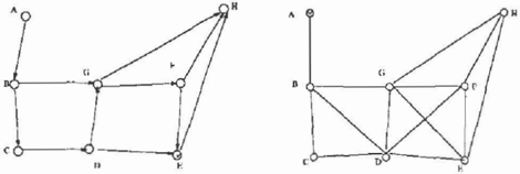
Example 6: If we define a criterion function whose components are singleton variables, then the complex­ ity bounds of optimization are identical to constraint satisfaction or finding the posterior probabilities. If we have the following criterion function defined on the belief network in Figure 1

then the augmented moral graph will have one addi­ tional edge connecting nodes A and G (see Figure 4(a), resulting in a primary clique-tree embedding in Figure 4(b) that differs from the tree in Figure 2( a).

5 CONCLUSIONS

We have shown that both constraint network process­ ing and belief network processing obey a time-space tradeoff based on structural properties that allow tai­ loring a combination of tree-clustering and cycle-cutset conditioning to certain time and space requirements. The same kind of tradeoff is obeyed by optimization problems when using the problem's graph augmented with arcs reflecting the structure of the criterion func­ tion.

Various algorithms that combine tree-clustering with conditioning were proposed in the past in the con­ text of constraint networks [Jegou, 1990] and belief networks [Darwiche, 1995; Peot and Shachter, 1991]. These algorithms are normally space linear (a point that is not always appreciated), and they seem to fall in the first tradeoff class, as they exploit singleton sep­ arators only. Our analysis presents a spectrum of algo­ rithms that will allow a richer time-space performance balance.

We would like to address breifly two questions. The first question is to what extent real-life problems pos­ sess structural properties that can be exploited by ei­ ther clustering, conditioning, or their hybrids. Recent empirical investigation using the domain of circuit di­ agnosisconfirm that the domain of circuit analysis can

benefit substantially from structure-based algorithms. The results are presented in a companion paper [Fat­ tah and Dechter, 1996}.

The second question is to what extent do worst-case bounds indeed reflect on average-case performance. Previous experimental work with clustering and condi­ tioning shows that while average-case performance of clustering methods correlates well with worst-case per­ formance, conditioning methods are sometimes much more effective than predicted by worst-case analysis. It is therefore necessary to implement and test the al­ gorithms implied by our analysis.

Acknowledgment

I would like to thank Rachel Ben-Eliyahu and Irina Rish for useful comments on the previous version of this paper. This work was partially supported by NSF grant IRI-91 57636, Air Force Office of S c ie n ti fi c Re­ search grant, AFOSR F49620-96-1-0224, and Rockwell MICRO grant #ACU-20755 and 95-043.

References

• [Arnborg et a/., 1 987] S.A. Arnborg, D.G. Corneil, and A. Proskurowski. Complexity of finding embed­ dings in a k-tree. SIAM Journal of Discrete Math­ ematics., 8:277-284, Hl87.
• [ A rn b o r g , 1 985] S.A. Arnborg. Efficient algorithms for combinatorial problems on graphs with bounded de­ composability - a survey. BIT, 25:2-23, 1985.
• [Bacchus and Grove, 1995] F Bacchus and A. Grove. Graphical models for preference and utility. In Un­ certainty in Artificial Intel ligence (U AI- 95), pages 3-10, 1 995.
• [ D. H. Krantz and Tversky, 1976] P. Suppes D. H. Krantz, R.D. Luce and A. T ve r ­ sky. Foundations of m e as u r eme n ts , academic press. 1 976.
• [Darwiche, 1995] A Darwiche. Conditioning a l g orithms for exact and approximate inference in causal networks. In Uncertainty in Artificial Intelligence (UAI-95), pages 99-107, 1995.
• [Dechter and Pearl, 1987] R. Dechter and J. Pearl. Network-based heuristics for constraint satisfaction problems. Artificial Intelligence, 34: 1-38, 1 987.
• [Dechter and Pearl, 1 989] R. Dechter and J. Pearl. Tree clustering for constraint networks. Artificial Intelligence, pages 353-366, 1989.
• [Dechter et a/. , 1 990] R. Dechter, A. Dechter, and J . Pearl. Optimization in constraint networks. In Influence Diagrams, Belief Nets and Deci.5ion Anal­ ysis, pages 41 1-425. John Wiley & Sons, Sussex, England, 1 990.
• [Dechter, 1 990] R. Dechter. Enhancement schems for constraint processing incorporating, backjumping, learning and c u ts e t decomposition. Artificial Intel­ ligence, 1 990 .
• [Dechter, 1 992] R. Dechter. Constraint networks. In S. Shapiro, editor, Encyclopedia of A rtificial Intelli­ gence, pages 276-285 . John Wiley & Sons, 1992.
• [Dechter, 1996] R. Dechter. Bucket elimination: A unif y i n g framework for probabilistic inference. In Uncertainty for Artificial Intelligence (UAI-96), 1 996.
• [Fattah and Dechter, 1996] Y.El . parameters for probabilistic reasoning: benchmark circuits. In Artificial Intelligence AI-96 , 1 996.
• Fattah and R. Dechter. An evaluation of structural results on Submitted to Uncertainty in (U )
• [Freuder, 1985] E. C. Freuder. A sufficient condition for backtrack-bounded search. Journal of the ACM, 34(4):755-761 , 1985.
• [Jegou, 1990] P Jegou. Cyclic c lus t e r in g : a compro­ mise between tree-clustering and the cycle-cutset method for improving search efficiency. In Euro­ pean Conference on AI (ECAI-90), pages 369-371, Stockholm, 1 990.
• [Jennsen and Jennsen, 1 994] F. Jennsen and F. Jennsen. Optimal junction trees. In Un­ certainty in A rtificial Intelligence {UAI-95}, pages 360-366, 1994.
• [Lauritzen and Spiegelhalter, 1988] S.L. Lauritzen and D .J . Spiegelhalter. Local computations with probabilities on graphical structures and their applications to expert systems. J. R. Stat. Soc., B 50: 1 27- 224, 1 988.
• [Mackworth and Freuder, 1985] A. K. Mackworth and E. C. Freuder. The complexity of some polynomial network consistency algorithms for constraint satis­ fac t i o n problems. Artificial Intelligence, 25( 1), 1985.
• [Pearl , 1986] J. Pearl. Fusion propagation and struc­ tu ri ng in belief networks. Artificial Intelligence, 29(3) :241-248, 1986.
• [Pearl, 1988] J. Pearl. Probabilistic Reasoning Intel­ ligent Systems. Morgan Kaoufmann, San Mateo, California, 1988.
• [Peat and Shachter, 1991] M.A. Peat and R.D. Shachter. Fusion and propagation with multiple observations i n belief networks. Artificial Intelligence, 48:299-318, 1991.
• [Shachter et al. , 1991] R.D. Shachter, S.K. Anderson, and P. Solovitz. Global conditioning for proba­ bilistic inference in belief networks. In Uncertainty in A rtificial Intel ligence (U AI-91 ) , pages 514-522, 1 99 1 .
• (Shachter, 1986] R.D. Shachter. Evaluating influence diagrams. Operations Research, 34(6), 1986.