Contents
0910.1266
Toward an automaton Constraint for Local Search
Jun He
Pierre Flener
Justin Pearson
Department of Information Technology Uppsala University, Box 337, SE - 751 05 Uppsala, Sweden
We explore the idea of using finite automata to implement new constraints for local search (this is already a successful technique in constraint-based global search). We show how it is possible to maintain incrementally the violations of a constraint and its decision variables from an automaton that describes a ground checker for that constraint. We establish the practicality of our approach idea on real-life personnel rostering problems, and show that it is competitive with the approach of [12].
1 Introduction
When a high-level constraint programming (CP) language lacks a (possibly global) constraint that would allow the formulation of a particular model of a combinatorial problem, then the modeller traditionally has the choice of (1) switching to another CP language that has all the required constraints, (2) formulating a different model that does not require the lacking constraints, or (3) implementing the lacking constraint in the low-level implementation language of the chosen CP language. This paper addresses the core question of facilitating the third option, and as a side effect often makes the first two options unnecessary.
The user-level extensibility of CP languages has been an important goal for over a decade. In the traditional global search approach to CP (namely heuristic-based tree search interleaved with propagation), higher-level abstractions for describing new constraints include indexicals [17]; (possibly enriched) deterministic finite automata (DFAs) via the automaton [2] and regular [11] generic constraints; and multivalued decision diagrams (MDDs) via the mdd [5] generic constraint. Usually, a generic but efficient propagation algorithm achieves a suitable level of local consistency by processing the higher-level description of the new constraint. In the more recent local search approach to CP (called constraint-based local search, CBLS, in [14]), higher-level abstractions for describing new constraints include invariants [9]; a subset of first-order logic with arithmetic via combinators [16] and differentiable invariants [15]; and existential monadic second-order logic for constraints on set decision variables [1]. Usually, a generic but incremental algorithm maintains the constraint and variable violations by processing the higher-level description of the new constraint.
In this paper, we revisit the description of new constraints via automata, already successfully tried within the global search approach to CP [2, 11], and show that it can also be successfully used within the local search approach to CP. The significance of this endeavour can be assessed by noting that 108 of the currently 313 global constraints in the Global Constraint Catalogue [3] are described by DFAs that are possibly enriched with counters and conditional transitions [2] (note that DFA generators can easily be written for other constraints, such as the pattern [4] and stretch [10] constraints, taking the necessarily ground parameters as inputs), so that all these constraints will instantly become available in CBLS once we show how to implement fully the enriched DFAs that are necessary for some of the described global constraints.
The rest of this paper is organised as follows. In Section 2, we present our algorithm for incrementally maintaining both the violation of a constraint described by an automaton, and the violations of
each decision variable of that constraint. In Section 3, we present experimental results establishing the practicality of our results, also in comparison to the prior approach of [12]. Finally, in Section 4, we summarise this work and discuss related as well as future work.
2 Incremental Violation Maintenance with Automata
In CBLS, three things are required of an implemented constraint: a method for calculating the violation of the constraint and each of its decision variables for the initial assignment (initialisation); a method for computing the differences of these violations upon a candidate local move (differentiability) to a neighbouring assignment; and a method for incrementally maintaining these violations when an actual move is made (incrementality). Intuitively, the higher the violation of a decision variable, the more can be gained by changing the value of that decision variable. It is essential to maintain incrementally the violations rather than recomputing them from scratch upon each local move, since by its nature a local search procedure will try many local moves to find one that ideally reduces the violation of the constraint or one of its decision variables.
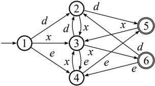
Our running example is the following, for a simple work scheduling constraint. There are values for two work shifts, day ( d ) and evening ( e ), as well as a value for enjoying a day off ( x ). Work shifts are subject to the following three conditions: one must take at least one day off before a change of work shift; one cannot work for more than two days in a row; and one cannot have more than two days off in a row. A DFA for checking ground instances of this constraint is given in Figure 1. The start state 1 is marked by a transition entering from nowhere, while the success states 5 and 6 are marked by double circles. Missing transitions, say from state 2 upon reading value e , are assumed to go to an implicit failure state, with a self-looping transition for every value (so that no success state is reachable from it).
2.1 Violations of a Constraint
To define and compute the violations of a constraint described by an automaton, we first introduce the notion of a segmentation of an assignment:
Definition 1 (Segmentation) Given an assignment V = 〈 d 1 , . . . , dn 〉 , a segmentation is a possibly empty sequence of non-empty sub-strings (referred to here as segments ) σ 1 , . . . , σ /lscript of d 1 · · · dn such that for each σ j = dp · · · dq and σ j + 1 = dr · · · ds we have that r > q.
For example, a possible segmentation of the assignment V = 〈 x , e , d , e , x , x 〉 is 〈 x , e 〉 , 〈 e , x , x 〉 ; note that the third character of the assignment is not part of any segment. In general, an assignment has multiple possible segmentations. We are interested in segmentations that are accepted by an automaton, in the following sense:
Definition 2 (Acceptance) Given an automaton and an assignment V = 〈 d 1 , . . . , dn 〉 , a segmentation σ 1 , . . . , σ /lscript is accepted by the automaton if there exist strings α 1 , . . . , α /lscript + 1 , where only α 1 and α /lscript + 1 may be empty, such that the concatenated string
is accepted by the automaton.
For example, given the automaton in Figure 1, the assignment V = 〈 x , e , d , e , x , x 〉 has a segmentation 〈 x , e 〉 , 〈 e , x , x 〉 with /lscript = 2, which is accepted by the automaton via the string 〈 x , e , x , e , x , x 〉 with α 1 = α 3 = ε (the empty string) and α 2 = 〈 d 〉 .
Given an assignment, the algorithm presented below initialises and updates a segmentation. The violations of the constraint and its decision variables are calculated relative to the current segmentation:
Definition 3 (Violations) Given an automaton describing a constraint c and given a segmentation σ 1 , . . . , σ /lscript of an assignment for a sequence of n decision variables V 1 , . . . , Vn:
- The constraint violation of c is n -∑ /lscript j = 1 | σ j | .
- The variable violation of decision variable Vi is 0 if there exists a segment index j in 1 , . . . , /lscript such that i ∈ σ j, and 1 otherwise.
It can easily be seen that the violation of a constraint is also the sum of the violations of its decision variables, and that it is never an underestimate of the minimal Hamming distance between the current assignment and any satisfying assignment.
Our approach, described in the next three sub-sections, greedily grows a segmentation from left to right across the current assignment relative to a satisfying assignment, and makes stochastic choices whenever greedy growth is impossible.
2.2 Initialisation
A finite automaton is first unrolled for a given length n of a sequence V = 〈 V 1 , . . . , Vn 〉 of decision variables, as in [11]:
Definition 4 (Layered Graph) Given a finite automaton with m states, the layered graph over a given number n of decision variables is a graph with m · ( n + 1 ) nodes. Each of the n + 1 vertical layers has a node for each of the m states of the automaton. The node for the start state of the automaton in layer 1 is marked as the start node. There is an arc labelled w from node f in layer i to node t in layer i + 1 if and only if there is a transition labelled w from f to t in the automaton. A node in layer n + 1 is marked as a success node if it corresponds to a success state in the automaton.
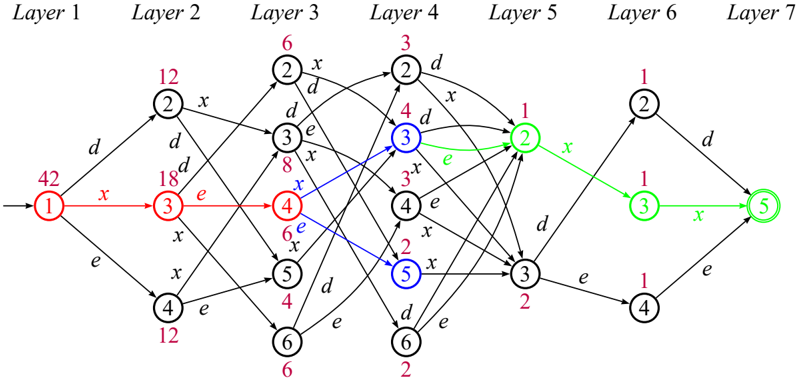
The layered graph is further processed by removing all nodes and arcs that do not lead to a success node. The resulting graph, seen as a DFA (or as an ordered MDD), need not be minimised (or reduced) for our approach (although this is a good idea for the global search approaches [2, 11], as argued in [7], and would be a good idea for the local search approach of [12]), as the number of arcs of the graph does not influence the time complexity of our algorithm below. For instance, the minimised unrolled version for n = 6 decision variables of the automaton in Figure 1 is given in Figure 2. Note that a satisfying assignment 〈 d 1 , . . . , dn 〉 corresponds to a path from the start node in layer 1 to a success node in layer n + 1, such that each arc from layer i to layer i + 1 of this path is labelled di .
Further, we require a number of data structures, where m is the number of states in the given automaton and n is the number of decision variables it was unrolled for:
- nbrPaths [ 1 ≤ i ≤ n , 1 ≤ j ≤ m ] records the number of paths from node j in layer i to a success node in the last layer; for example, see the numbers by each node in Figure 2;
- /lscript is the number of segments in the current segmentation;
- segments σ 1 , . . . , σ /lscript record the current segmentation;
- Violation [ 1 ≤ i ≤ n ] records the current violation of decision variable Vi (see Definition 3);
The nbrPaths matrix can be computed in straightforward fashion by dynamic programming. The other three data structures are initialised (when the starting position is s = 1) and maintained (when decision variable Vs is changed, with s ≥ 1) by the calcSegment ( s ) procedure of Algorithm 1. Upon some initialisations (lines 2 and 3), it (re)visits only the decision variables Vs , . . . , Vn (line 4). If the value of the currently visited decision variable Vi triggers the extension of the currently last segment (lines 6 and 9) or the creation of a new segment (lines 6 to 9), then its violation is 0 (line 10). Otherwise, its violation is 1 and a successor node is picked with a probability weighted according to the number of paths from the current node to a success node (lines 11 to 14). Toward this, we maintain the nodes of the picked path (line 16).
The time complexity of Algorithm 1 is linear in the number n of decision variables, because only one path (from layer s to layer n + 1) is explored, with a constant-time effort at each node. Once the pre-processing is done, the time complexity of Algorithm 1 is thus independent of the number of arcs of the unrolled automaton! Hence the minimisation (or reduction) of the unrolled automaton would be merely for space savings (and for the convenience of human reading) as well as for accelerating the preprocessing computation of the nbrPaths matrix. In our experiments, these space and time savings are not warranted by the time required for minimisation (or reduction).
Note that this algorithm works without change or loss of performance on non -deterministic finite automata (NFAs). This is potentially interesting since NFAs are often smaller than their equivalent DFAs, but (as just seen) the number of arcs has no influence on the time complexity of Algorithm 1.
Algorithm 1 Computation and update of the current segmentation from position s
1: procedure calcSegment ( s : 1 , . . . , n ) 2: let /lscript be the number of segments picked for 〈 V 1 , . . . , Vs -1 〉 at the previous run; assume /lscript = 0 at the first run 3: node [ 1 ] ← 1; inSegment ← true 4: for all i ← s to n do 5: if the current value, say a , of Vi is the label of an arc from node [ i ] to some node t then 6: if not inSegment then 7: /lscript ← /lscript + 1; σ /lscript ← ε ; inSegment ← true { c } reate a new segment 8: end if 9: σ /lscript ← σ /lscript · a 10: Violation [ i ] ← 0 11: else 12: inSegment ← false 13: Violation [ i ] ← 1 14: pick a successor t of node [ i ] with probability nbrPaths [ i + 1 , t ] / nbrPaths [ i , node [ i ]] 15: end if 16: node [ i + 1 ] ← t 17: end forFor example, in Figure 2, with the initial assignment V = 〈 x , e , d , e , x , x 〉 and a first call to Algorithm 1 with s = 1, the first segment will be 〈 x , e 〉 (the red path). Next, the assignment V 3 = d triggers a violation of 1 for decision variable V 3 (we say that it is a violated variable ) because there is no arc labelled d that connects the current node 4 in layer 3 with any nodes in layer 4. However, node 4 in layer 3 has two out-going arcs, namely to nodes 3 and 5 in layer 4 (in blue). In layer 4, there are 4 paths from node 3 to the last layer, compared to 2 such paths from node 5, so node 3 is picked with probability 4 6 and node 5 is picked with probability 2 6 (where the 2, 4, and 6 are the purple numbers by those nodes), and we assume that node 3 in layer 4 is picked. From there, we get the second segment 〈 e , x , x 〉 (the green path), which stops at success node 5 in the last layer. The violation of the constraint is thus 1, because the value of one decision variable does not participate in any segment.
Continuing the example, we assume now that decision variable V 3 is changed to value e , and hence we call Algorithm 1 with s = 3. Only /lscript = 1 segment can be kept from the previous segmentation picked for 〈 V 1 , V 2 〉 , namely 〈 x , e 〉 (the red path). Since there is an arc labelled e from the current node 4 in layer 3, namely to node 5 in layer 4, segment /lscript is extended (line 9) to 〈 x , e , e 〉 . However, with decision variable V 4 still having value e , this segment cannot be extended further, since there is no arc labelled e from node 5 in layer 4, and hence V 4 is violated. Similarly, decision variables V 5 = x and V 6 = x are violated no matter which successors are picked, so no new segment is ever created. The violation of the constraint is thus 3 because the value of three decision variables do not participate in any segment. Hence changing decision variable V 3 from value d to value e would not be considered a good local move, as the constraint violation increases from 1 to 3. Changing decision variable V 3 to value x instead would be a much better local move, as the first segment 〈 x , e 〉 is then extended to the entire current assignment 〈 x , e , d , e , x , x 〉 , without detecting any violated variables, so that the violation of the constraint is then 0, meaning that a satisfying assignment was found.
In Section 3, we experiment with a deterministic method [12] for picking the next node and experimentally show that our random pick is computationally quicker at finding solutions.
| Mon | Tue | Wed | Thu | Fri | Sat | Sun |
|---|---|---|---|---|---|---|
| x | x | x | d | d | d | d |
| x | x | e | e | e | x | x |
| d | d | d | x | x | e | e |
| e | e | x | x | n | n | n |
| n | n | n | n | x | x | x |
2.3 Differentiability
At present, the differences of the (constraint and variable) violations upon a candidate local move are calculated na¨ ıvely by first making the candidate move and th en undoing it.
2.4 Incrementality
Local search proceeds from the current assignment by checking a number of neighbours of that assignment and picking a neighbour that ideally reduces the violation: the exact heuristics are often problem dependent. But in order to make local search computationally efficient, the violations of the constraint and its decision variables have to be computed in an incremental fashion whenever a decision variable changes value. As shown in Subsection 2.2, our initialisation Algorithm 1 can also be invoked with an arbitrary starting position s when decision variable Vs is assigned a new value.
We have implemented this algorithm in Comet [14], an object-oriented CP language with among others a CBLS back-end (available at www.dynadec.com ).
3 Experiments
We now establish the practicality of the proposed violation maintenance algorithm by experimenting with it. All local search experiments were conducted under Comet (version 2.0 beta) on an Intel 2.4 GHz Linux machine with 512 MB memory while the constraint programming examples where implemented using SICStus Prolog.
Many industries and services need to function around the clock. Rotating schedules such as the one in Table 1 (a real-life example taken from [8]) are a popular way of guaranteeing a maximum of equity to the involved work teams (see [8]). In our first benchmark, there are day ( d ), evening ( e ), and night ( n ) shifts of work, as well as days off ( x ). Each team works maximum one shift per day. The scheduling horizon has as many weeks as there are teams. In the first week, team i is assigned to the schedule in row i . For any next week, each team moves down to the next row, while the team on the last row moves up to the first row. Note how this gives almost full equity to the teams, except, for instance, that team 1 does not enjoy the six consecutive days off that the other teams have, but rather three consecutive days off at the beginning of week 1 and another three at the end of week 5. The daily workload may be uniform: for instance, in Table 1, each day has exactly one team on-duty for each work shift, and two teams entirely off-duty; we denote this as ( 1 d , 1 e , 1 n , 2 x ) ; assuming the work shifts average 8h, each employee will work 7 · 3 · 8 = 168h over the five-week-cycle, or 33 . 6h per week. Daily workload, whether uniform or not, can be enforced by global cardinality ( gcc ) constraints [13] on the columns. Further, any number of consecutive workdays must be between two and seven, and any change in work shift can only occur after
Algorithm 2 The search procedure
1: void search(var{int}[] V, ConstraintSystemtwo to seven days off. This can be enforced by a pattern ( X , { ( d , x ) , ( e , x ) , ( n , x ) , ( x , d ) , ( x , e ) , ( x , n ) } ) constraint [4] and a circular stretch ( X , [ d , e , n , x ] , [ 2 , 2 , 2 , 2 ] , [ 7 , 7 , 7 , 7 ]) constraint [10] on the table flattened row-wise into a sequence X .
Our model posts the pattern and stretch constraints described by automata. The gcc constraints on the columns of the matrix are kept invariant: the first assignment is chosen so as to satisfy them, and then only swap moves inside a column are considered. As a meta-heuristic, we use tabu search with restarting. At each iteration, the search procedure in Algorithm 2 selects a violated variable x (line 4; recall that the violation of a decision variable is here at most 1) and another variable y of distinct value in the same column so that their swap (line 8) gives the greatest violation change (lines 5 to 7). The length of the tabu list is the maximum between 6 and the sum of the violations of all constraints (lines 9 and 10). The best solution so far is maintained (lines 11 to 14). Restarting is done every 2 · | X | iterations (lines 15 and 16). The expressions for the length of the tabu list and the restart criterion were experimentally determined.
Recall that Algorithm 1 computes a greedy random segmentation; hence it might give different segmentations when used for probing a swap and when used for actually performing that swap. Therefore, we record the segmentation of each swap probe, and at the actual swap we just apply its recorded segmentation.
We ran experiments over the eight instances from ( 2 d , 1 e , 1 n , 2 x ) to ( 16 d , 8 e , 8 n , 16 x ) (we write the latter as ( 2 d , 1 e , 1 n , 2 x ) · 8) with uniform daily workload, where the weekly workload is 37 . 3h. For example, instance ( 2 d , 1 e , 1 n , 2 x ) · 3 has the uniform daily workload of 2 · 3 teams on the day shift, 1 · 3 teams on the evening shift, 1 · 3 teams on the night shift, and 2 · 3 teams off-duty. Table 2 gives statistics on the run times and numbers of iterations to find the first solutions over 100 runs from random initial assignments.
Posting the product of the pattern and stretch automata (accepting the intersection of their two reg-
| optimisation time (ms) | number of iterations | |||||||
|---|---|---|---|---|---|---|---|---|
| instance | min | max | avg | σ | min | max | avg | σ |
| ( 2 d , 1 e , 1 n , 2 x ) · 1 | 6 | 100 | 22 | 20 | 9 | 528 | 115 | 108 |
| ( 2 d , 1 e , 1 n , 2 x ) · 2 | 12 | 692 | 168 | 154 | 32 | 2484 | 585 | 561 |
| ( 2 d , 1 e , 1 n , 2 x ) · 3 | 32 | 2588 | 688 | 611 | 44 | 6612 | 1726 | 1571 |
| ( 2 d , 1 e , 1 n , 2 x ) · 4 | 80 | 6553 | 1199 | 1275 | 86 | 11212 | 2125 | 2303 |
| ( 2 d , 1 e , 1 n , 2 x ) · 5 | 60 | 9373 | 1417 | 1545 | 72 | 15604 | 2292 | 2556 |
| ( 2 d , 1 e , 1 n , 2 x ) · 6 | 160 | 5901 | 1527 | 1227 | 161 | 8051 | 2051 | 1681 |
| ( 2 d , 1 e , 1 n , 2 x ) · 7 | 176 | 9896 | 1720 | 1686 | 157 | 11680 | 1966 | 1981 |
| ( 2 d , 1 e , 1 n , 2 x ) · 8 | 216 | 12472 | 2620 | 2309 | 150 | 12588 | 2603 | 2354 |
| optimisation time (ms) | number of iterations | |||||||
|---|---|---|---|---|---|---|---|---|
| instance | min | max | avg | σ | min | max | avg | σ |
| ( 2 d , 1 e , 1 n , 2 x ) · 1 | 1 | 16 | 2 | 3 | 6 | 61 | 11 | 9 |
| ( 2 d , 1 e , 1 n , 2 x ) · 2 | 1 | 64 | 12 | 12 | 13 | 235 | 34 | 46 |
| ( 2 d , 1 e , 1 n , 2 x ) · 3 | 12 | 76 | 25 | 13 | 21 | 173 | 46 | 29 |
| ( 2 d , 1 e , 1 n , 2 x ) · 4 | 28 | 172 | 51 | 27 | 32 | 297 | 72 | 49 |
| ( 2 d , 1 e , 1 n , 2 x ) · 5 | 28 | 200 | 79 | 42 | 34 | 286 | 106 | 61 |
| ( 2 d , 1 e , 1 n , 2 x ) · 6 | 56 | 368 | 135 | 76 | 61 | 487 | 156 | 101 |
| ( 2 d , 1 e , 1 n , 2 x ) · 7 | 84 | 768 | 188 | 123 | 69 | 848 | 189 | 140 |
| ( 2 d , 1 e , 1 n , 2 x ) · 8 | 112 | 764 | 233 | 112 | 72 | 736 | 202 | 113 |
ular languages) has been experimentally determined to be more efficient than posting the two automata individually, hence all experiments in this paper use the product automaton.
Further improvements can be achieved by using a non-random initial assignment. Table 3 gives statistics on the run times and numbers of iterations to find the first solutions over 100 runs, where the initial assignment of instance ( 2 d , 1 e , 1 n , 2 x ) · i consists of i copies of Table 4. The results show that this non-random initialisation provides a better starting point. Although much more experimentation is required, these initial results show that even on the instance ( 2 d , 1 e , 1 n , 2 x ) · 8 with 336 decision variables it is possible to find solutions quickly.
The only related work we are aware of is a Comet implementation [12] of the regular constraint [11], based on the ideas for the propagator of the soft regular constraint [6]. The difference is that they estimate the violation change compared to the nearest solution (in terms of Hamming distance from the current assignment), whereas we estimate it compared to one randomly picked solution. In our terminology (although it is not implemented that way in [12]), they find a segmentation, such that an accepting string for the automaton has the minimal Hamming distance to the current assignment.
Tables 5 and 6 give comparisons between (our re-implementation of) regular [12], our method, and
| Mon | Tue | Wed | Thu | Fri | Sat | Sun |
|---|---|---|---|---|---|---|
| d | d | d | d | d | d | d |
| e | e | e | e | e | e | e |
| n | n | n | n | n | n | n |
| x | x | x | x | x | x | x |
| d | d | d | d | d | d | d |
| x | x | x | x | x | x | x |
| optimisation time (ms) | number of iterations | ||||||||
|---|---|---|---|---|---|---|---|---|---|
| instance | our method | regular [12] | CP | our method | regular [12] | ||||
| avg | σ | avg | σ | avg | σ | avg | σ | ||
| ( 2 d , 1 e , 1 n , 2 x ) · 1 | 22 | 20 | 395 | 378 | 10 | 115 | 108 | 98 | 100 |
| ( 2 d , 1 e , 1 n , 2 x ) · 2 | 168 | 154 | 1584 | 1187 | 10 | 585 | 561 | 223 | 170 |
| ( 2 d , 1 e , 1 n , 2 x ) · 3 | 688 | 611 | 3441 | 2871 | 10 | 1726 | 1571 | 333 | 287 |
| ( 2 d , 1 e , 1 n , 2 x ) · 4 | 1199 | 1275 | 5584 | 4423 | 40 | 2125 | 2303 | 399 | 319 |
| ( 2 d , 1 e , 1 n , 2 x ) · 5 | 1417 | 1545 | 8828 | 7606 | 100 | 2292 | 2556 | 514 | 444 |
| ( 2 d , 1 e , 1 n , 2 x ) · 6 | 1527 | 1227 | 13888 | 10863 | 510 | 2051 | 1681 | 672 | 529 |
| ( 2 d , 1 e , 1 n , 2 x ) · 7 | 1720 | 1686 | 13170 | 9814 | 3520 | 1966 | 1981 | 536 | 485 |
| ( 2 d , 1 e , 1 n , 2 x ) · 8 | 2620 | 2309 | 20202 | 11530 | 25820 | 2603 | 2354 | 745 | 602 |
| St Louis Police | 12740 | 11199 | 50261 | 48026 | - | 20287 | 17952 | 3248 | 2498 |
a SICStus Prolog constraint program (CP) where the product automaton of the pattern and stretch constraints was posted using the built-in propagation-based implementation of the automaton constraint [2]. These experiments show:
- Compared with regular [12], our method has a higher number of iterations, as it is more stochastic. However, our run times are lower, as our cost of one iteration is much smaller (linear in the number of decision variables, instead of linear in the number of arcs of the unrolled automaton).
- Compared with the CP method, both local search methods need more time to find the first solution when the number of weeks is small. However, when the number of weeks increases, the runtime of CP increases sharply. From the instance ( 2 d , 1 e , 1 n , 2 x ) · 7, the runtime of CP exceeds the average runtime of our method. From the instance ( 2 d , 1 e , 1 n , 2 x ) · 8, the runtime of CP exceeds also the average runtime of regular [12].
Besides the rotating nurse instances, we ran experiments on another, harder real-life scheduling instance. The St Louis Police problem (described in [12]) has a seventeen-week-cycle; however it has more constraints than the rotating nurse problem. It has non-uniform daily workloads. For example, on Mondays, five teams work during the day, five at night, four in the evening, and three teams enjoy a day off; while on Sundays, three teams work during the day, four at night, four in the evening, and six teams
| optimisation time (ms) | number of iterations | |||||||
|---|---|---|---|---|---|---|---|---|
| instance | our method | regular [12] | our method | regular [12] | ||||
| avg | σ | avg | σ | avg | σ | avg | σ | |
| ( 2 d , 1 e , 1 n , 2 x ) · 1 | 2 | 3 | 44 | 26 | 11 | 9 | 10 | 7 |
| ( 2 d , 1 e , 1 n , 2 x ) · 2 | 12 | 12 | 182 | 65 | 34 | 46 | 22 | 9 |
| ( 2 d , 1 e , 1 n , 2 x ) · 3 | 25 | 13 | 478 | 201 | 46 | 29 | 41 | 17 |
| ( 2 d , 1 e , 1 n , 2 x ) · 4 | 51 | 27 | 834 | 254 | 72 | 49 | 56 | 18 |
| ( 2 d , 1 e , 1 n , 2 x ) · 5 | 79 | 42 | 1546 | 876 | 106 | 61 | 87 | 51 |
| ( 2 d , 1 e , 1 n , 2 x ) · 6 | 135 | 76 | 2414 | 1233 | 156 | 101 | 113 | 59 |
| ( 2 d , 1 e , 1 n , 2 x ) · 7 | 188 | 123 | 4517 | 3276 | 189 | 140 | 181 | 134 |
| ( 2 d , 1 e , 1 n , 2 x ) · 8 | 233 | 112 | 4473 | 1958 | 202 | 113 | 160 | 71 |
| St Louis Police | 3990 | 4012 | 67159 | 55632 | 5389 | 5598 | 3949 | 3159 |
enjoy a day off. Any number of consecutive workdays must be between three and eight, and any change in work shift can only occur after two to seven days off. The problem has other vertical constraints; for example, no team can work in the same shift on four consecutive Mondays. Further, the problem has complex pattern constraints that limit possible changes of work shifts; for example, only the patterns ( d , x , d ) , ( e , x , e ) , ( n , x , n ) , ( d , x , e ) , ( e , x , n ) , and ( n , x , d ) are allowed. For this hard real-life problem, our method still works well: experimental results can also be found in Tables 5 and 6.
It is possible to post (see Figure 3) the constraints of the rotating nurse problem using the differentiable invariants [15] of Comet . This is possible in general for any automaton by encoding all the paths to a success state by using Comet 's conjunction and disjunction combinators. As the automata get larger, these expressions can become too large to post, and even when it is possible to post these expressions our current experiments show that our approach is more efficient.
4 Conclusion
In summary, we have shown that the idea of describing novel constraints by automata can be successfully imported from classical (global search) constraint programming to constraint-based local search (CBLS). Our violation algorithms take time linear in the number of decision variables, whereas the propagation algorithms take amortised time linear in the number of arcs of the unrolled automaton [2, 11]. We have also experimentally shown that our approach is competitive with the CBLS approach of [12].
There is of course a trade-off between using an automaton to describe a constraint and using a handcrafted implementation of that constraint. On the one hand, a hand-crafted implementation of a constraint is normally more efficient during search, because properties of the constraint can be exploited, but it may take a lot of time to implement and verify it. On the other hand, the (violation or propagation) algorithm processing the automaton is implemented and verified once and for all, and our assumption is that it takes a lot less time to describe and verify a new constraint by an automaton than to implement and verify its algorithm. We see thus opportunities for rapid prototyping with constraints described by automata: once a sufficiently efficient model, heuristic, and meta-heuristic have been experimentally determined with
Figure 3: A model for the unrolled DFA in Figure 2 with Comet combinators
its help, some extra efficiency may be achieved, if necessary, by hand-crafting implementations of any constraints described by automata.
As witnessed in our experiments, constraint composition (by conjunction) is easy to experiment with under the DFA approach, as there exist standard and efficient algorithms for composing and minimising DFAs, but there is no known systematic way of composing violation (or propagation) algorithms when decomposition is believed to obstruct efficiency.
In the global search approach to CP, the common modelling device of reification can be used to shrink the size of DFAs describing constraints [2]. For instance, consider the element ([ x 1 , . . . , xn ] , i , v ) constraint, which holds if and only if xi = v . Upon reifying the decision variables x 1 , . . . , xn into new Boolean decision variables b 1 , . . . , bn such that xi = v ⇔ bi = 1, it suffices to pose the automaton ([ b 1 , . . . , bn ] , DFA ) constraint, where DFA corresponds to the regular expression 0 ∗ 1 ( 0 + 1 ) ∗ , meaning that at least one 1 must be found in the sequence of the bi decision variables. However, such explicit reification constraints are not necessary in constraint-based local search, as a total assignment of values to all decision variables is maintained at all times: instead of processing the values of the decision variables when computing the segments, one can process their reified values .
It has been shown that the use of counters (initialised at the start state and evolving during possibly conditional transitions) to enrich the language of DFAs and thereby shrink the size of DFAs can be handled in the global search approach to CP [2], possibly upon some concessions at the level of local consistency that can be achieved. In the Global Constraint Catalogue [3], some 31 of the currently 108 constraints described by DFAs use lists of counters, and another 25 constraints use arrays of counters. We need to investigate the effects on our violation maintenance algorithm of introducing counters and conditional transitions.
Acknowledgements
The authors are supported by grant 2007-6445 of the Swedish Research Council (VR), and Jun He is also supported by grant 2008-611010 of China Scholarship Council and the National University of Defence Technology of China. Many thanks to Magnus ˚ Agren (SICS) for some useful discussions on this work, and to the anonymous referees of both LSCS'09 and the Doctoral Programme of CP'09, especially for pointing out the existence of [12, 6].
References
- Magnus ˚ Agren, Pierre Flener & Justin Pearson (2007): Generic incremental algorithms for local search . Constraints 12(3), pp. 293-324. (Collects the results of papers at CP-AI-OR'05 , CP'05 , and CP'06 , published in LNCS 3524, 3709, and 4204).
- Nicolas Beldiceanu, Mats Carlsson & Thierry Petit (2004): Deriving filtering algorithms from constraint checkers . In: Mark Wallace, editor: Proceedings of CP'04, LNCS 3258. Springer-Verlag, pp. 107-122.
- Nicolas Beldiceanu, Mats Carlsson & Jean-Xavier Rampon (2007): Global constraint catalogue: Past, present, and future . Constraints 12(1), pp. 21-62. Dynamic on-line version at www.emn.fr/x-info/ sdemasse/gccat . Long version as Technical Report T2005:08, Swedish Institute of Computer Science, November 2005.
- St´ ephane Bourdais, Philippe Galinier & Gilles Pesant (2003): HIBISCUS: A constraint programming application to staff scheduling in health care . In: Francesca Rossi, editor: Proceedings of CP'03, LNCS 2833. Springer-Verlag, pp. 153-167.
- Kenil C. K. Cheng & Roland H. C. Yap (2008): Maintaining generalized arc consistency on ad hoc r-ary constraints . In: Peter J. Stuckey, editor: Proceedings of CP'08, LNCS 5202. Springer-Verlag, pp. 509-523.
- Willem-Jan van Hoeve, Gilles Pesant & Louis-Martin Rousseau (2006): On global warming: Flow-based soft global constraints . Journal of Heuristics 12(4-5), pp. 347-373.
- Mikael Z. Lagerkvist (2008): Techniques for Efficient Constraint Propagation . Technical Report, KTH - The Royal Institute of Technology, Stockholm, Sweden. Licentiate Thesis.
- Gilbert Laporte (1999): The art and science of designing rotating schedules . Journal of the Operational Research Society 50(10), pp. 1011-1017.
- Laurent Michel & Pascal Van Hentenryck (1997): Localizer: A modeling language for local search . In: Gert Smolka, editor: Proceedings of CP'97, LNCS 1330. Springer-Verlag, pp. 237-251.
- Gilles Pesant (2001): A filtering algorithm for the stretch constraint . In: Toby Walsh, editor: Proceedings of CP'01, LNCS 2239. Springer-Verlag, pp. 183-195.
- Gilles Pesant (2004): A regular language membership constraint for finite sequences of variables . In: Mark Wallace, editor: Proceedings of CP'04, LNCS 3258. Springer-Verlag, pp. 482-495.
- Benoit Pralong (2007): Impl´ ementation de la contrainte Regular en Comet . Master's thesis, ´ Ecole Polytechnique de Montr´ eal, Canada.
- Jean-Charles R´ egin (1996): Generalized arc-consistency for global cardinality constraint . In: Proceedings of AAAI'96. AAAI Press, pp. 209-215.
- Pascal Van Hentenryck & Laurent Michel (2005): Constraint-Based Local Search . The MIT Press.
- Pascal Van Hentenryck & Laurent Michel (2006): Differentiable invariants . In: Fr´ ed´ eric Benhamou, editor: Proceedings of CP'06, LNCS 4204. Springer-Verlag, pp. 604-619.
- Pascal Van Hentenryck, Laurent Michel & Liyuan Liu (2004): Constraint-based combinators for local search . In: Mark Wallace, editor: Proceedings of CP'04, LNCS 3258. Springer-Verlag, pp. 47-61.
- Pascal Van Hentenryck, Vijay Saraswat & Yves Deville (1993): Design, implementation, and evaluation of the constraint language cc(FD) . Technical Report CS-93-02, Brown University, Providence, USA. Revised
version in Journal of Logic Programming 37(1-3):293-316, 1998. Based on the unpublished manuscript Constraint Processing in cc(FD) , 1991.