Uncertainty in Soft Temporal Constraint Problems: A General Framework and Controllability Algorithms for The Fuzzy Case

Francesca Rossi Kristen Brent Venable

University of Padova, Department of Pure and Applied Mathematics, Via Trieste, 63 35121 PADOVA ITALY

Neil Yorke-Smith

SRI International,

333 Ravenswood Ave, Menlo Park, CA 94025 USA

Abstract

In real-life temporal scenarios, uncertainty and preferences are often essential and coexisting aspects. We present a formalism where quantitative temporal constraints with both preferences and uncertainty can be defined. We show how three classical notions of controllability (that is, strong, weak, and dynamic), which have been developed for uncertain temporal problems, can be generalized to handle preferences as well. After defining this general framework, we focus on problems where preferences follow the fuzzy approach, and with properties that assure tractability. For such problems, we propose algorithms to check the presence of the controllability properties. In particular, we show that in such a setting dealing simultaneously with preferences and uncertainty does not increase the complexity of controllability testing. We also develop a dynamic execution algorithm, of polynomial complexity, that produces temporal plans under uncertainty that are optimal with respect to fuzzy preferences.

1. Introduction

Current research on temporal constraint reasoning, once exposed to the difficulties of real-life problems, can be found lacking both expressiveness and flexibility. In rich application domains it is often necessary to simultaneously handle not only temporal constraints, but also preferences and uncertainty.

This need can be seen in many scheduling domains. The motivation for the line of research described in this paper is the domain of planning and scheduling for NASA space missions. NASA has tackled many scheduling problems in which temporal constraints have been used with reasonable success, while showing their limitations in their lack of capability to deal with uncertainty and preferences. For example, the Remote Agent (Rajan, Bernard, Dorais, Gamble, Kanefsky, Kurien, Millar, Muscettola, Nayak, Rouquette, Smith, Taylor, & Tung, 2000; Muscettola, Morris, Pell, & Smith, 1998) experiments, which consisted of placing an AI system on-board to plan and execute spacecraft activities, represents one of the most interesting examples of this. Remote Agent worked with high level goals which specified, for example, the duration and frequency of time windows within which the spacecraft had to take asteroid images to be used for orbit determination for the on-board navigator. Remote Agent dealt with both flexible time intervals and uncontrollable events; however, it did not deal with preferences: all the temporal constraints are hard. The benefit of adding preferences to this framework would be to allow the planner to handle uncontrollable events while at the same time maximizing the mission manager's preferences.

[email protected]

[email protected]

[email protected]

A more recent NASA application is in the rovers domain (Dearden, Meuleau, Ramakrishnan, Smith, & Washington, 2002; Bresina, Jonsson, Morris, & Rajan, 2005). NASA is interested in the generation of optimal plans for rovers designed to explore a planetary surface (e.g. Spirit and Opportunity for Mars) (Bresina et al., 2005). Dearden et al. (2002) describe the problem of generating plans for planetary rovers that handle uncertainty over time and resources. The approach involves first constructing a 'seed' plan, and then incrementally adding contingent branches to this plan in order to improve its utility. Again, preferences could be used to embed utilities directly in the temporal model.

A third space application, which will be used several times in this paper as a running example, concerns planning for fleets of Earth Observing Satellites (EOS) (Frank, Jonsson, Morris, & Smith, 2001). This planning problem involves multiple satellites, hundreds of requests, constraints on when and how to serve each request, and resources such as instruments, recording devices, transmitters and ground stations. In response to requests placed by scientists, image data is acquired by an EOS. The data can be either downlinked in real time or recorded on board for playback at a later time. Ground stations or other satellites are available to receive downlinked images. Different satellites may be able to communicate only with a subset of these resources, and transmission rates will differ from satellite to satellite and from station to station. Further, there may be different financial costs associated with using different communication resources. In (Frank et al., 2001) the EOS scheduling problem is dealt with by using a constraint-based interval representation. Candidate plans are represented by variables and constraints, which reflect the temporal relationship between actions and the constraints on the parameters of states or actions. Also, temporal constraints are necessary to model duration and ordering constraints associated with the data collection, recording, and downlinking tasks. Solutions are preferred based on objectives (such as maximizing the number of high priority requests served, maximizing the expected quality of the observations, and minimizing the cost of downlink operations). Uncertainty is present due to weather: specifically due to duration and persistence of cloud cover, since image quality is obviously affected by the amount of clouds over the target. In addition, some of the events that need to be observed may happen at unpredictable times and have uncertain durations (e.g. fires or volcanic eruptions).

Someexisting frameworks, such as Simple Temporal Problems with Preferences (STPPs) (Khatib, Morris, Morris, & Rossi, 2001), address the lack of expressiveness of hard temporal constraints by adding preferences to the temporal framework, but do not take into account uncertainty. Other models, such as Simple Temporal Problems with Uncertainty (STPUs) (Vidal & Fargier, 1999), account for contingent events, but have no notion of preferences. In this paper we introduce a framework which allows us to handle both preferences and uncertainty in Simple Temporal Problems. The proposed model, called Simple Temporal Problems with Preferences and Uncertainty (STPPUs), merges the two pre-existing models of STPPs and STPUs.

AnSTPPUinstance represents a quantitative temporal problem with preferences and uncertainty via a set of variables, representing the starting or ending times of events (which can be controllable by the agent or not), and a set of soft temporal constraints over such variables, each of which includes an interval containing the allowed durations of the event or the allowed times between events. Apreference function associating each element of the interval with a value specifies how much that value is preferred. Such soft constraints can be defined on both controllable and uncontrollable events. In order to further clarify what is modeled by an STPPU, let us emphasize that graduality is only allowed in terms of preferences and not of uncertainty. In this sense, the uncertainty represented by contingent STPPU constraints is the same as that of contingent STPU constraints: all

durations are assumed to be equally possible. In addition to expressing uncertainty, in STPPUs, contingent constraints can be soft and different preference levels can be associated to different durations of contingent events.

On these problems, we consider notions of controllability similar to those defined for STPUs, to be used instead of consistency because of the presence of uncertainty, and we adapt them to handle preferences. These notions, usually called strong , weak , and dynamic controllability, refer to the possibility of 'controlling' the problem, that is, of the executing agent assigning values to the controllable variables, in a way that is optimal with respect to what Nature has decided, or will decide, for the uncontrollable variables. The word optimal here is crucial, since in STPUs, where there are no preferences, we just need to care about controllability, and not optimality. In fact, the notions we define in this paper that directly correspond to those for STPUs are called strong, weak, and dynamic optimal controllability.

After defining these controllability notions and proving their properties, we then consider the same restrictions which have been shown to make temporal problems with preferences tractable (Khatib et al., 2001; Rossi, Sperduti, Venable, Khatib, Morris, & Morris, 2002), i.e, semi-convex preference functions and totally ordered preferences combined with an idempotent operator. In this context, for each of the above controllability notions, we give algorithms that check whether they hold, and we show that adding preferences does not make the complexity of testing such properties worse than in the case without preferences. Moreover, dealing with different levels of preferences, we also define testing algorithms which refer to the possibility of controlling a problem while maintaining a preference of at least a certain level (called α -controllability). Finally, in the context of dynamic controllability, we also consider the execution of dynamic optimal plans.

Parts of the content of this paper have appeared in (Venable & Yorke-Smith, 2003; Rossi, Venable, & Yorke-Smith, 2003; Yorke-Smith, Venable, & Rossi, 2003; Rossi, Venable, & Yorke-Smith, 2004). This paper extends the previous work in at least two directions. First, while in those papers optimal and α controllability (strong or dynamic) were checked separately, now we can check optimal (strong or dynamic) controllability and, if it does not hold, the algorithm will return the highest α such that the given problem is α -strong or α -dynamic controllable. Moreover, results are presented in a uniform technical environment, by providing a thorough theoretical study of the properties of the algorithms and their computational aspects, which makes use of several unpublished proofs.

This paper is structured as follows. In Section 2 we give the background on temporal constraints with preference and with uncertainty. In Section 3 we define our formalism for Simple Temporal Problems with both preferences and uncertainty and, in Section 4, we describe our new notions of controllability. Algorithms to test such notions are described respectively in Section 5 for Optimal Strong Controllability, in Section 6 for Optimal Weak Controllability, and in Section 7 for Optimal Dynamic Controllability. In Section 8 we then give a general strategy for using such notions. Finally, in Section 9, we discuss related work, and in Section 10 we summarize the main results and we point out some directions for future developments. To make the paper more readable, the proofs of all theorems are contained in the Appendix.

2. Background

In this section we give the main notions of temporal constraints (Dechter, Meiri, & Pearl, 1991) and the framework of Temporal Constraint Satisfaction Problems with Preferences (TCSPPs) (Khatib

et al., 2001; Rossi et al., 2002), which extend quantitative temporal constraints (Dechter et al., 1991) with semiring-based preferences (Bistarelli, Montanari, & Rossi, 1997). We also describe Simple Temporal Problems with Uncertainty (STPUs) (Vidal & Fargier, 1999; Morris, Muscettola, & Vidal, 2001), which extend a tractable subclass of temporal constraints to model agent-uncontrollable contingent events, and we define the corresponding notions of controllability, introduced in (Vidal &Fargier, 1999).

2.1 Temporal Constraint Satisfaction Problems

One of the requirements of a temporal reasoning system for planning and scheduling problems is an ability to deal with metric information; in other words, to handle quantitative information on duration of events (such as 'It will take from ten to twenty minutes to get home'). Quantitative temporal networks provide a convenient formalism to deal with such information. They consider instantaneous events as the variables of the problem, whose domains are the entire timeline. A variable may represent either the beginning or an ending point of an event, or a neutral point of time. An effective representation of quantitative temporal networks, based on constraints, is within the framework of Temporal Constraint Satisfaction Problems (TCSPs) (Dechter et al., 1991).

In this paper we are interested in a particular subclass of TCSPs, known as Simple Temporal Problems (STPs) (Dechter et al., 1991). In such a problem, a constraint between time-points X i and X j is represented in the constraint graph as an edge X i → X j , labeled by a single interval [ a ij , b ij ] that represents the constraint a ij ≤ X j -X i ≤ b ij . Solving an STP means finding an assignment of values to variables such that all temporal constraints are satisfied.

Whereas the complexity of a general TCSP comes from having more than one interval in a constraint, STPs can be solved in polynomial time. Despite the restriction to a single interval per constraint, STPs have been shown to be valuable in many practical applications. This is why STPs have attracted attention in the literature.

An STP can be associated with a directed weighted graph G d = ( V, E d ) , called the distance graph . It has the same set of nodes as the constraint graph but twice the number of edges: for each binary constraint over variables X i and X j , the distance graph has an edge X i → X j which is labeled by weight b ij , representing the linear inequality X j -X i ≤ b ij , as well as an edge X j → X i which is labeled by weight -a ij , representing the linear inequality X i -X j ≤ -a ij .

Each path from X i to X j in the distance graph G d , say through variables X i 0 = X i , X i 1 , X i 2 , . . . , X i k = X j induces the following path constraint : X j -X i ≤ ∑ k h =1 b i h -1 i h . The intersection of all induced path constraints yields the inequality X j -X i ≤ d ij , where d ij is the length of the shortest path from X i to X j , if such a length is defined, i.e. if there are no negative cycles in the distance graph. An STP is consistent if and only if its distance graph has no negative cycles (Shostak, 1981; Leiserson & Saxe, 1988). This means that enforcing path consistency, by an algorithm such as PC-2 , is sufficient for solving STPs (Dechter et al., 1991). It follows that a given STP can be effectively specified by another complete directed graph, called a d -graph , where each edge X i → X j is labeled by the shortest path length d ij in the distance graph G d .

In (Dechter et al., 1991) it is shown that any consistent STP is backtrack-free (that is, decomposable) relative to the constraints in its d -graph . Moreover, the set of temporal constraints of the form [ -d ji , d ij ] is the minimal STP corresponding to the original STP and it is possible to find one of its solutions using a backtrack-free search that simply assigns to each variable any value that satisfies the minimal network constraints compatibly with previous assignments. Two specific solu-

tions (usually called the latest and the earliest assignments) are given by S L = { d 01 , . . . , d 0 n } and S E = { d 10 , . . . , d n 0 } , which assign to each variable respectively its latest and earliest possible time (Dechter et al., 1991).

The d -graph (and thus the minimal network ) of an STP can be found by applying FloydWarshall's All Pairs Shortest Path algorithm (Floyd, 1962) to the distance graph with a complexity of O ( n 3 ) where n is the number of variables. If the graph is sparse, the Bellman-Ford Single Source Shortest Path algorithm can be used instead, with a complexity equal to O ( nE ) , where E is the number of edges. We refer to (Dechter et al., 1991; Xu & Choueiry, 2003) for more details on efficient STP solving.

2.2 Temporal CSPs with Preferences

Although expressive, TCSPs model only hard temporal constraints. This means that all constraints have to be satisfied, and that the solutions of a constraint are all equally satisfying. However, in many real-life situations some solutions are preferred over others and, thus, the global problem is to find a way to satisfy the constraints optimally, according to the preferences specified.

To address this need, the TCSP framework has been generalized in (Khatib et al., 2001) to associate each temporal constraint with a preference function which specifies the preference for each distance allowed by the constraint. This framework merges TCSPs and semiring-based soft constraints (Bistarelli et al., 1997).

Definition 1 (soft temporal constraint) A soft temporal constraint is a 4-tuple 〈{ X,Y } , I, A, f 〉 consisting of

• a set of two variables { X,Y } over the integers, called the scope of the constraint;
• a set of disjoint intervals I = { [ a 1 , b 1 ] , . . . , [ a n , b n ] } , where a i , b i ∈ Z , and a i ≤ b i for all i = 1 , . . . , n ;
• a set of preferences A ;
• a preference function f : I → A , which is a mapping of the elements of I into preference values, taken from the set A .

Given an assignment of the variables X and Y , X = v x and Y = v y , we say that this assignment satisfies the constraint 〈{ X,Y } , I, A, f 〉 iff there exists [ a i , b i ] ∈ I such that a i ≤ v y -v x ≤ b i . In such a case, the preference associated with the assignment by the constraint is f ( v y -v x ) = p . /Box

When the variables and the preference set of an STPP are apparent, we will omit them and write a soft temporal constraint just as a pair 〈 I, f 〉 .

Following the soft constraint approach (Bistarelli et al., 1997), the preference set is the carrier of an algebraic structure known as a c-semiring . Informally a c-semiring S = 〈 A, + , × , 0 , 1 〉 is a set equipped with two operators satisfying some proscribed properties (for details, see Bistarelli et al., 1997)). The additive operator + is used to induce the ordering on the preference set A ; given two elements a, b ∈ A , a ≥ b iff a + b = a . The multiplicative operator × is used to combine preferences.

Definition 2 (TCSPP) Given a semiring S = 〈 A, + , × , 0 , 1 〉 , a Temporal Constraint Satisfaction Problems with Preferences (TCSPP) over S is a pair 〈 V, C 〉 , where V is a set of variables and C is a set of soft temporal constraint over pairs of variables in V and with preferences in A . /Box

Definition 3 (solution) Given a TCSPP 〈 V, C 〉 over a semiring S , a solution is a complete assignment of the variables in V . A solution t is said to satisfy a constraint c in C with preference p if the projection of t over the pair of variables of c 's scope satisfies c with preference p . We will write pref ( t, c ) = p . /Box

Each solution has a global preference value , obtained by combining, via the × operator, the preference levels at which the solution satisfies the constraints in C .

Definition 4 (preference of a solution) Given a TCSPP 〈 V, C 〉 over a semiring S , the preference of a solution t = 〈 v 1 , . . . , v n 〉 , denoted val ( t ) , is computed by Π c ∈ C pref ( s, c ) . /Box

The optimal solutions of a TCSPP are those solutions which have the best global preference value, where 'best' is determined by the ordering ≤ of the values in the semiring.

Definition 5 (optimal solutions) Given a TCSPP P = 〈 V, C 〉 over the semiring S , a solution t of P is optimal if for every other solution t ′ of P , t ′ /negationslash≥ S t . /Box

Choosing a specific semiring means selecting a class of preferences. For example, the semiring

allows one to model the so-called fuzzy preferences (Ruttkay, 1994; Schiex, 1992), which associate to each element allowed by a constraint a preference between 0 and 1 (with 0 being the worst and 1 being the best preferences), and gives to each complete assignment the minimal among all preferences selected in the constraints. The optimal solutions are then those solutions with the maximal preference. Another example is the semiring S CSP = 〈{ false, true } , ∨ , ∧ , f alse, true 〉 , which allows one to model classical TCSPs, without preferences, in the more general TCSPP framework.

In this paper we will refer to fuzzy temporal constraints. However, the absence of preferences in some temporal constraints can always be modelled using just the two elements 0 and 1 in such constraints. Thus preferences can always coexists with hard constraints.

Aspecial case occurs when each constraint of a TCSPP contains a single interval. In analogy to what is done in the case without preferences, such problems are called Simple Temporal Problems with Preferences (STPPs). This class of temporal problems is interesting because, as noted above, STPs are polynomially solvable while general TCSPs are NP-hard, and the computational effect of adding preferences to STPs is not immediately obvious.

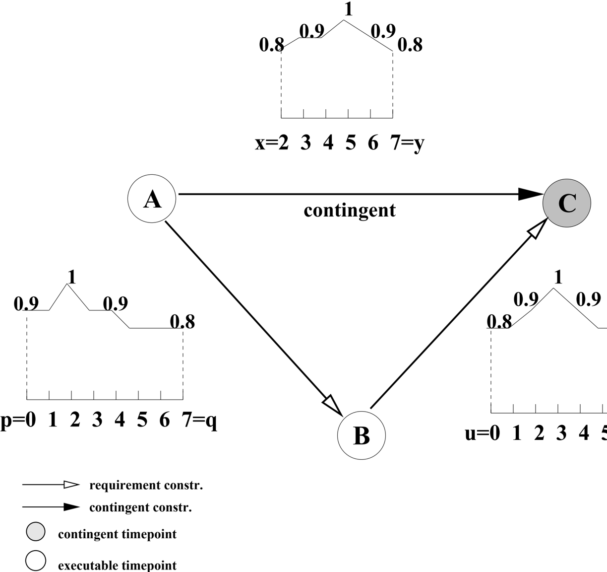
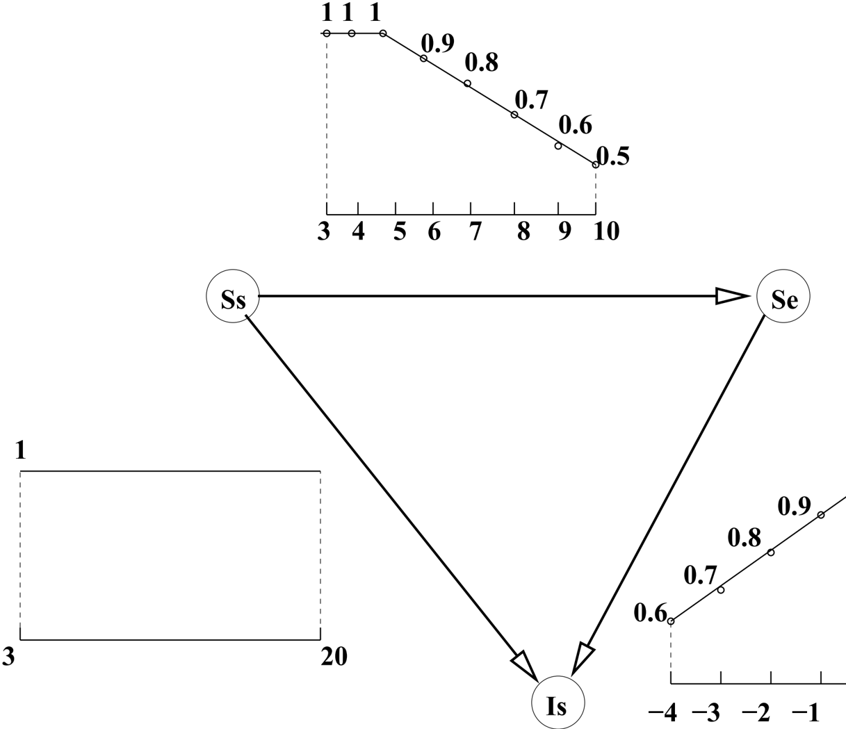
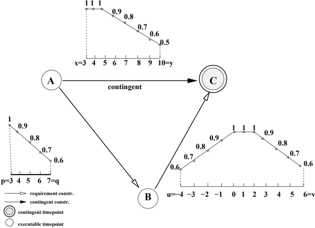
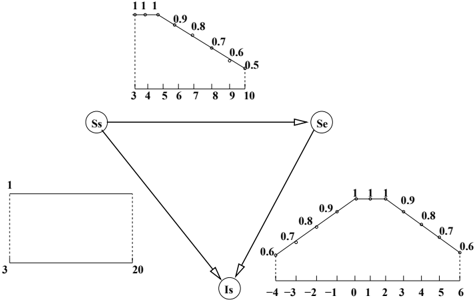
Example 1 Consider the EOS example given in Section 1. In Figure 1 we show an STPP that models the scenario in which there are three events to be scheduled on a satellite: the start time ( Ss ) and ending time ( Se ) of a slewing procedure and the starting time ( Is ) of an image retrieval. The slewing activity in this example can take from 3 to 10 units of time, ideally between 3 to 5 units of time, and the shortest time possible otherwise. The image taking can start any time between 3 and 20 units of time after the slewing has been initiated. The third constraint, on variables Is and Se , models the fact that it is better for the image taking to start as soon as the slewing has stopped. /Box

In the following example, instead, we consider an STPP which uses the set-based semiring: S set = 〈 ℘ ( A ) , ∪ , ∩ , ∅ , A 〉 . Notice that, as in the fuzzy semiring, the multiplicative operator, i.e., intersection, is idempotent, while the order induced by the additive operator, i.e., union, is partial.

Example 2 Consider a scenario where three friends, Alice, Bob, and Carol, want to meet for a drink and then for dinner and must decide at what time to meet and where to reserve dinner depending on how long it takes to get to the restaurant. The variables involved in the problem are: the global start time X 0 , with only the value 0 in its domain, the start time of the drink ( Ds ), the time to leave for dinner ( De ), and the time of arrival at the restaurant ( Rs ). They can meet, for the drink, between 8 and 9:00pm and they will leave for dinner after half an hour. Moreover, depending on the restaurant they choose, it will take from 20 to 40 minutes to get to dinner. Alice prefers to meet early and have dinner early, like Carol. Bob prefers to meet at 8:30 and to go to the best restaurant which is the farthest. Thus, we have the following two soft temporal constraints. The first constraint is defined on the variable pair ( X 0 , Ds ) , the interval is [8:00,9:00] and the preference function, f s , is such that, f s (8 : 00) = { Alice, Carol } , f s (8 : 30) = { Bob } and f s (9 : 00) = ∅ . The second constraint is a binary constraint on pair ( De , Rs ), with interval [20 , 40] and preference function f se , such that, f se (20) = { Alice, Carol } and f se (20) = ∅ and f se (20) = { Bob } . There is an additional 'hard' constraint on the variable pair ( Ds,De ) , which can be modeled by the interval [30 , 30] and a single preference equal to { Alice, Carol, Bob } . The optimal solution is ( X 0 = 0 , Ds = 8 : 00 , De = 8 : 30 , Rs = 8 : 50) , with preference { Alice, Carol } . /Box

Although both TCSPPs and STPPs are NP-hard, in (Khatib et al., 2001) a tractable subclass of STPPs is described. The tractability assumptions are: the semi-convexity of preference functions, the idempotence of the combination operator of the semiring, and a totally ordered preference set. Apreference function f of a soft temporal constraint 〈 I, f 〉 is semi-convex iff for all y ∈ /Rfractur + , the set { x ∈ I, f ( x ) ≥ y } forms an interval. Notice that semi-convex functions include linear, convex, and also some step functions. The only aggregation operator on a totally ordered set that is idempotent is min (Dubois & Prade, 1985), i.e. the combination operator of the S FCSP semiring.

If such tractability assumptions are met, STPPs can be solved in polynomial time. In (Rossi et al., 2002) two polynomial solvers for this tractable subclass of STPPs are proposed. One solver is

based on the extension of path consistency to TCSPPs. The second solver decomposes the problem into solving a set of hard STPs.

2.3 Simple Temporal Problems with Uncertainty

When reasoning concerns activities that an agent performs interacting with an external world, uncertainty is often unavoidable. TCSPs assume that all activities have durations under the control of the agent. Simple Temporal Problems with Uncertainty (STPUs) (Vidal & Fargier, 1999) extend STPs by distinguishing contingent events, whose occurrence is controlled by exogenous factors often referred to as 'Nature'.

As in STPs, activity durations in STPUs are modelled by intervals. The start times of all activities are assumed to be controlled by the agent (this brings no loss of generality). The end times, however, fall into two classes: requirement (free' inVidal & Fargier, 1999) and contingent . The former, as in STPs, are decided by the agent, but the agent has no control over the latter: it only can observe their occurrence after the event; observation is supposed to be known immediately after the event. The only information known prior to observation of a time-point is that nature will respect the interval on the duration. Durations of contingent links are assumed to be independent.

In an STPU, the variables are thus divided into two sets depending on the type of time-points they represent.

Definition 6 (variables) The variables of an STPU are divided into:

• executable time-points : are those points, b i , whose time is assigned by the executing agent;
• contingent time-points : are those points, e i , whose time is assigned by the external world. /Box

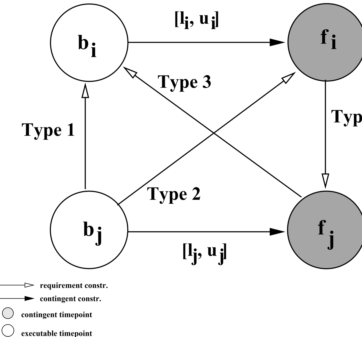
The distinction on variables leads to constraints which are also divided into two sets, requirement and contingent, depending on the type of variables they constrain. Note that as in STPs all the constraints are binary. Formally:

Definition 7 The constraints of an STPU are divided into:

• a requirement constraint (or link) r ij , on generic time-points t i and t j 1 , is an interval I ij = [ l ij , u ij ] such that l ij ≤ γ ( t j ) -γ ( t i ) ≤ u ij where γ ( t i ) is a value assigned to variable t i
• a contingent link g hk , on executable point b h and contingent point e k , is an interval I hk = [ l ij , u ij ] which contains all the possible durations of the contingent event represented by b h and e k . /Box

The formal definition of an STPU is the following:

Definition 8 (STPU) A Simple Temporal Problem with Uncertainty (STPU) is a 4-tuple N = { X e , X c , R r , R c } such that:

• X e = { b 1 , . . . , b n e } : is the set of executable time-points;
• X c = { e 1 , . . . , e n c } : is the set of contingent time-points;

1. In general t i and t j can be either contingent or executable time-points.

• R r = { c i 1 j 1 , . . . , c i C j C } : is the set C of requirement constraints;
• R c = { g i 1 j 1 , . . . , g i G j G } : is the set G of contingent constraints. /Box

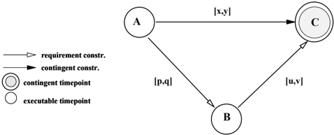
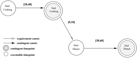
Example 3 This is an example taken from (Vidal & Fargier, 1999), which describes a scenario which can be modeled using an STPU. Consider two activities Cooking and Having dinner . Assume you don't want to eat your dinner cold. Also, assume you can control when you start cooking and when the dinner starts but not when you finish cooking or when the dinner will be over. The STPU modeling this example is depicted in Figure 2. There are two executable time-points { Startcooking, Start-dinner } and two contingent time-points { End-cooking, End-dinner } . Moreover, the contingent constraint on variables { Start-cooking, End-cooking } models the uncontrollable duration of fixing dinner which can take anywhere from 20 to 40 minutes; the contingent constraint on variables { Start-dinner, End-dinner } models the uncontrollable duration of the dinner that can last from 30 to 60 minutes. Finally, there is a requirement constraint on variables { End-cooking, Startdinner } that simply bounds to 10 minutes the time between when the food is ready and when the dinner starts. /Box

Assignments to executable variables and assignments to contingent variables are distinguished:

Definition 9 (control sequence) A control sequence δ is an assignment to executable time-points. It is said to be partial if it assigns values to a proper subset of the executables, otherwise complete . /Box

Definition 10 (situation) Asituation ω is a set of durations on contingent constraints. If not all the contingent constraints are assigned a duration it is said to be partial , otherwise complete . /Box

Definition 11 (schedule) A schedule is a complete assignment to all the time-points in X e and X c . A schedule T identifies a control sequence, δ T , consisting of all the assignments to the executable time-points, and a situation, ω T , which is the set of all the durations identified by the assignments in T on the contingent constraints. Sol ( P ) denotes the set of all schedules of an STPU. /Box

It is easy to see that to each situation corresponds an STP. In fact, once the durations of the contingent constraints are fixed, there is no more uncertainty in the problem, which becomes an STP, called the underlying STP . This is formalized by the notion of projection .

Definition 12 (projection) A projection P ω , corresponding to a situation ω , is the STP obtained leaving all requirement constraints unchanged and replacing each contingent constraint g hk with

the constraint 〈 [ ω hk , ω hk ] 〉 , where ω hk is the duration of event represented by g hk in ω . Proj ( P ) is the set of all projections of an STPU P . /Box

2.4 Controllability

It is clear that in order to solve a problem with uncertainty all possible situations must be considered. The notion of consistency defined for STPs does not apply since it requires the existence of a single schedule, which is not sufficient in this case since all situations are equally possible. 2 For this reason, in (Vidal & Fargier, 1999), the notion of controllability has been introduced. Controllability of an STPU is, in some sense, the analogue of consistency of an STP. Controllable means the agent has a means to execute the time-points under its control, subject to all constraints. The notion of controllability is expressed, in terms of the ability of the agent to find, given a situation, an appropriate control sequence. This ability is identified with having a strategy:

Definition 13 (strategy) A strategy S is a map S : Proj ( P ) → Sol ( P ) , such that for every projection P ω , S ( P ω ) is a schedule which induces the durations in ω on the contingent constraints. Further, a strategy is viable if, for every projection P ω , S ( P ω ) is a solution of P ω . /Box

We will write [ S ( P ω )] x to indicate the value assigned to executable time-point x in schedule S ( P ω ) , and [ S ( P ω )] <x the history of x in S ( P ω ) , that is, the set of durations of contingent constraints which occurred in S ( P ω ) before the execution of x , i.e. the partial solution so far.

In (Vidal & Fargier, 1999), three notions of controllability are introduced for STPUs.

2.4.1 STRONG CONTROLLABILITY

The first notion is, as the name suggests, the most restrictive in terms of the requirements that the control sequence must satisfy.

Definition 14 (Strong Controllability) An STPU P is Strongly Controllable (SC) iff there is an execution strategy S s.t. ∀ P ω ∈ Proj ( P ) , S ( P ω ) is a solution of P ω , and [ S ( P 1 )] x = [ S ( P 2 )] x , ∀ P 1 , P 2 projections and for every executable time-point x . /Box

In words, an STPU is strongly controllable if there is a fixed execution strategy that works in all situations. This means that there is a fixed control sequence that will be consistent with any possible scenario of the world. Thus, the notion of strong controllability is related to that of conformant planning. It is clearly a very strong requirement. As Vidal and Fargier (1999) suggest, SC may be relevant in some applications where the situation is not observable at all or where the complete control sequence must be known beforehand (for example in cases in which other activities depend on the control sequence, as in the production planning area).

In (Vidal & Fargier, 1999) a polynomial time algorithm for checking if an STPU is strongly controllable is proposed. The main idea is to rewrite the STPU given in input as an equivalent STP only on the executable variables. What is important to notice, for the contents of this paper, is that algorithm StronglyControllable takes in input an STPU P = { X e , X c , R r , R c } and returns in output an STP defined on variables X e . The STPU in input is strongly controllable iff the derived STP is consistent. Moreover, every solution of the STP is a control sequence which guarantees

2. Tsamardinos (2002) has augmented STPUs to include probability distributions over the possible situations; in this paper we implicitly assume a uniform, independent distribution on each link.

strong controllability for the STPU. When the STP is consistent, the output of StronglyControllable is its minimal form.

In (Vidal & Fargier, 1999) it is shown that the complexity of StronglyControllable is O ( n 3 ) , where n is the number of variables.

2.4.2 WEAK CONTROLLABILITY

On the other hand, the notion of controllability with the fewest restrictions on the control sequences is Weak Controllability.

Definition 15 (Weak Controllability) An STPU P is said to be Weakly Controllable (WC) iff ∀ P ω ∈ Proj ( P ) there is a strategy S ω s.t. S ω ( P ω ) is a solution of P ω . /Box

In words, an STPU is weakly controllable if there is a viable global execution strategy: there exists at least one schedule for every situation. This can be seen as a minimum requirement since, if this property does not hold, then there are some situations such that there is no way to execute the controllable events in a consistent way. It also looks attractive since, once an STPU is shown to WC, as soon as one knows the situation, one can pick out and apply the control sequence that matches that situation. Unfortunately in (Vidal & Fargier, 1999) it is shown that this property is not so useful in classical planning. Nonetheless, WC may be relevant in specific applications (as largescale warehouse scheduling) where the actual situation will be totally observable before (possibly just before ) the execution starts, but one wants to know in advance that, whatever the situation, there will always be at least one feasible control sequence.

In (Vidal & Fargier, 1999) it is conjectured and in (Morris & Muscettola, 1999) it is proven that the complexity of checking weak controllability is co-NP-hard. The algorithm proposed for testing WC in (Vidal & Fargier, 1999) is based on a classical enumerative process and a lookahead technique.

Strong Controllability implies Weak Controllability (Vidal & Fargier, 1999). Moreover, an STPU can be seen as an STP if the uncertainty is ignored. If enforcing path consistency removes some elements from the contingent intervals, then these elements belong to no solution. If so, it is possible to conclude that the STPU is not weakly controllable.

Definition 16 (pseudo-controllability) An STPU is pseudo-controllable if applying path consistency leaves the intervals on the contingent constraints unchanged. /Box

Unfortunately, if path consistency leaves the contingent intervals untouched, we cannot conclude that the STPU is weakly controllable. That is, WC implies pseudo-controllability but the converse is false. In fact, weak controllability requires that given any possible combination of durations of all contingent constraints the STP corresponding to that projection must be consistent. Pseudo-controllability, instead, only guarantees that for each possible duration on a contingent constraint there is at least one projection that contains such a duration and it is a consistent STP.

2.4.3 DYNAMIC CONTROLLABILITY

In dynamic applications domains, such as planning, the situation is observed over a time. Thus decisions have to be made even if the situation remains partially unknown. Indeed the distinction between Strong and Dynamic Controllability is equivalent to that between conformant and conditional planning. The final notion of controllability defined in (Vidal & Fargier, 1999) address this

Pseudocode of DynamicallyControllable

1. input STPU W;
2. If Wis not pseudo-controllable then write 'not DC' and stop ;
3. Select all triangles ABC, C uncontrollable, A before C, such that the upper bound of the BC interval, v , is non-negative.
4. Introduce any tightenings required by the Precede case and any waits required by the Unordered case.
5. Do all possible regressions of waits, while converting unconditional waits to lower bounds. Also introduce lower bounds as provided by the general reduction.
6. If steps 3 and 4 do not produce any new (or tighter)
7. constraints, then return true, otherwise go to 2.

Figure 4: A triangular STPU.

case. Here we give the definition provided in (Morris et al., 2001) which is equivalent but more compact.

Definition 17 (Dynamic Controllability) An STPU P is Dynamically Controllable (DC) iff there is a strategy S such that ∀ P 1 , P 2 in Proj ( P ) and for any executable time-point x :

1. S ( P 1 ) is a solution of P 1 and S ( P 2 ) is a solution of P 2 . /Box

In words, an STPU is dynamically controllable if there exists a viable strategy that can be built, step-by-step, depending only the observed events at each step. SC = ⇒ DC and that DC = ⇒ WC. Dynamic Controllability, seen as the most useful controllability notion in practice, is also the one that requires the most complicated algorithm. Surprisingly, Morris et al. (2001) and Morris and Muscettola (2005) proved DC is polynomial in the size of the STPU representation. In Figure 3 the pseudocode of algorithm DynamicallyControllable is shown.

In this paper we will extend the notion of dynamic controllability in order to deal with preferences. The algorithm we will propose to test this extended property will require a good (even if not complete) understanding of the DynamicallyControllable algorithm. Thus, we will now give the necessary details on this algorithm.

As it can be seen, the algorithm is based on some considerations on triangles of constraints. The triangle shown in Figure 4 is a triangular STPU with one contingent constraint, AC, two executable time-points, A and B, and a contingent time-point C. Based on the sign of u and v , three different cases can occur:

• Follow case ( v < 0 ): B will always follow C. If the STPU is path consistent then it is also DC since, given the time at which C occurs after A, by definition of path consistency, it is always possible to find a consistent value for B.
• Precede case ( u ≥ 0 ): B will always precede or happen simultaneously with C. Then the STPU is dynamically controllable if y -v ≤ x -u , and the interval [ p, q ] on AB should be replaced by interval [ y -v, x -u ] , that is by the sub-interval containing all the elements of [ p, q ] that are consistent with each element of [ x, y ] .
• Unordered case ( u < 0 and v ≥ 0 ): B can either follow or precede C. To ensure dynamic controllability, B must wait either for C to occur first, or for t = y -v units of time to go by after A. In other words, either C occurs and B can be executed at the first value consistent with C's time, or B can safely be executed t units of time after A's execution. This can be described by an additional constraint which is expressed as a wait on AB and is written < C,t > , where t = y -v . Of course if x ≥ y -v then we can raise the lower bound of AB, p , to y -v ( Unconditional Unordered Reduction ), and in any case we can raise it to x if x > p ( General Unordered reduction ) .

It can be shown that waits can be propagated (in Morris et al., 2001, the term 'regressed'is used ) from one constraint to another: a wait on AB induces a wait on another constraint involving A, e.g. AD, depending on the type of constraint DB. In particular, there are two possible ways in which the waits can be regressed.

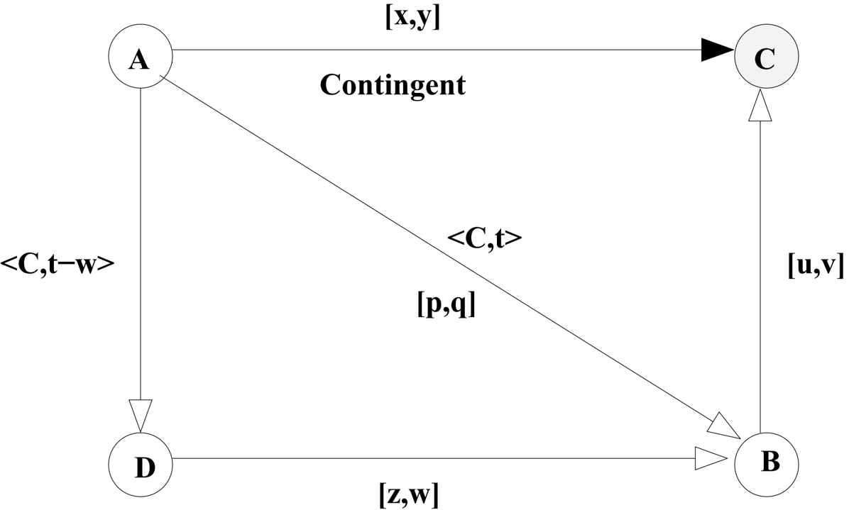
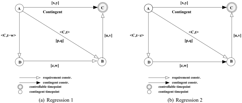
• Regression 1: assume that the AB constraint has a wait 〈 C,t 〉 . Then, if there is any DB constraint (including AB itself) with an upper bound, w , it is possible to deduce a wait 〈 C,t -w 〉 on AD . Figure 5(a) shows this type of regression.

/negationslash

• Regression 2: assume that the AB constraint has a wait 〈 C,t 〉 , where t ≥ 0 . Then, if there is a contingent constraint DB with a lower bound, z , and such that B = C , it is possible to deduce a wait 〈 C,t -z 〉 on AD . Figure 5(b) shows this type of regression.

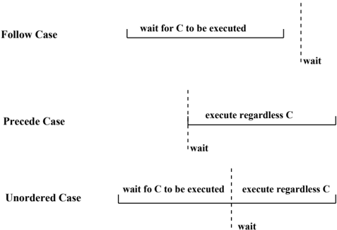
Assume for simplicity and without loss of generality that A is executed at time 0. Then, B can be executed before the wait only if C is executed first. After the wait expires, B can safely be executed at any time left in the interval. As Figure 6 shows, it is possible to consider the Follow and Precede cases as special cases of the Unordered. In the Follow case we can put a 'dummy' wait after the end of the interval, meaning that B must wait for C to be executed in any case (Figure 6 (a)). In the Precede case, we can set a wait that expires at the first element of the interval meaning that B will be executed before C and any element in the interval will be consistent with C (Figure 6 (b)). The Unordered case can thus be seen as a combination of the two previous states. The part of the interval before the wait can be seen as a Follow case (in fact, B must wait for C until the wait expires), while the second part including and following the wait can be seen as a Precede case (after the wait has expired, B can be executed and any assignment to B that corresponds to an element of this part of interval AB will be consistent with any possible future value assigned to C).

Figure 5: Regressions in algorithm DynamicallyControllable .

wait

Figure 6: The resulting AB interval constraint in the three cases considered by the DynamicallyControllable algorithm.

The DynamicallyControllable algorithm applies these rules to all triangles in the STPU and regresses all possible waits. If no inconsistency is found, that is no requirement interval becomes empty and no contingent interval is squeezed, the STPU is DC and the algorithm returns an STPU where some constraints may have waits to satisfy, and the intervals contain elements that appear in at least one possible dynamic strategy. This STPU can then be given to an execution algorithm which dynamically assigns values to the executables according to the current situation.

The pseudocode of the execution algorithm, DC-Execute , is shown in Figure 7. The execution algorithm observes, as the time goes by, the occurrence of the contingent events and accordingly executes the controllables. For any controllable B, its execution is triggered if it is (1) live , that is, if current time is within its bounds, it is (2) enabled , that is, all the executables constrained to

Pseudocode for DC-Execute

1. input STPU P ;
2. Perform initial propagation from the start time-point;
3. repeat
4. immediately execute any executable time-points that have reached their upper bounds;
5. arbitrarily pick an executable time-point x that is live and enabled and not yet executed, and whose waits, if any, have all been satisfied;
6. execute x ;
7. propagate the effect of the execution;
8. if network execution is complete then return;
9. else advance current time, propagating the effect of any contingent time-points that occur; 10. until false;

Figure 7: Algorithm that executes a dynamic strategy for an STPU.

happen before have occurred, and (3) all the waits imposed by the contingent time-points on B have expired.

DC-Execute produces dynamically a consistent schedule on every STPU on which algorithm DynamicallyControllable reports success (Morris et al., 2001). The complexity of the algorithm is O ( n 3 r ) , where n is the number of variables and r is the number of elements in an interval. Since the polynomial complexity relies on the assumption of a bounded maximum interval size, Morris et al. (2001) conclude that DynamicallyControllable is pseudopolynomial. A DC algorithm of 'strong' polynomial complexity is presented in (Morris & Muscettola, 2005). The new algorithm differs from the previous one mainly because it manipulates the distance graph rather than the constraint graph of the STPU. It's complexity is O ( n 5 ) . What is important to notice for our purposes is that, from the distance graph produced in output by the new algorithm, it is possible to directly recover the intervals and waits of the STPU produced in output by the original algorithm described in (Morris et al., 2001).

3. Simple Temporal Problems with Preferences and Uncertainty (STPPUs)

Consider a temporal problem that we would model naturally with preferences in addition to hard constraints, but one also features uncertainty. Neither an STPP nor an STPU is adequate to model such a problem. Therefore we propose what we will call Simple Temporal Problems with Preferences and Uncertainty , or STPPUs for short.

Intuitively, an STPPU is an STPP for which time-points are partitioned into two classes, requirement and contingent, just as in an STPU. Since some time-points are not controllable by the agent, the notion of consistency of an STP(P) is replaced by that of controllability, just as in an STPU. Every solution to the STPPU has a global preference value, just as in an STPP, and we seek a solution which maximizes this value, while satisfying controllability requirements.

More precisely, we can extend some definitions given for STPPs and STPUs to fit STPPUs in the following way.

Definition 18 In a context with preferences:

• an executable time-point is a variable, x i , whose time is assigned by the agent;
• a contingent time-point is a variable, e i , whose time is assigned by the external world;
• a soft requirement link r ij , on generic time-points t i and t j 3 , is a pair 〈 I ij , f ij 〉 , where I ij = [ l ij , u ij ] such that l ij ≤ γ ( t j ) -γ ( t i ) ≤ u ij where γ ( t i ) is a value assigned to variable t i , and f ij : I ij → A is a preference function mapping each element of the interval into an element of the preference set, A , of the semiring S = 〈 A, + , × , 0 , 1 〉 ;
• a soft contingent link g hk , on executable point b h and contingent point e k , is a pair 〈 I hk , f hk 〉 where interval I hk = [ l hk , u hk ] contains all the possible durations of the contingent event represented by b h and e k and f hk : I hk → A is a preference function that maps each element of the interval into an element of the preference set A . /Box

In both types of constraints, the preference function represents the preference of the agent on the duration of an event or on the distance between two events. However, while for soft requirement constraints the agent has control and can be guided by the preferences in choosing values for the time-points, for soft contingent constraints the preference represents merely a desire of the agent on the possible outcomes of Nature: there is no control on the outcomes. It should be noticed that in STPPUs uncertainty is modeled, just like in STPUs, assuming 'complete ignorance' on when events are more likely to happen. Thus, all durations of contingent events are assumed to be equally possible (or plausible) and different levels of plausibility are not allowed.

We can now state formally the definition of STPPUs, which combines preferences from the definition of an STPP with contingency from the definition of an STPU.

Definition 19 (STPPU) A Simple Temporal Problem with Preferences and Uncertainty (STPPU) is a tuple P = ( N e , N c , L r , L c , S ) where:

• N e is the set of executable time-points;
• N c is the set of contingent time-points;
• S = 〈 A, + , × , 0 , 1 〉 is a c-semiring;
• L r is the set of soft requirement constraints over S;
• L c is the set of soft contingent constraints over S. /Box

Note that, as STPPs, also STPPUs can model hard constraints by soft constraints in which each element of the interval is mapped into the maximal element of the preference set. Further, without loss of generality, and following the assumptions made for STPUs (Morris et al., 2001), we assume that no two contingent constraints end at the same time-point.

Once we have a complete assignment to all time-points we can compute its global preference, as in STPPs. This is done according to the semiring-based soft constraint schema: first we project the assignment on each soft constraint, obtaining an element of the interval and the preference

3. Again, in general t i and t j can be either contingent or executable time-points.

associated to that element; then we combine the preferences obtained on all constraints with the multiplicative operator of the semiring. Given two assignments with their preference, the best is chosen using the additive operator. An assignment is optimal if there is no other assignment with a preference which is better in the semiring's ordering.

In the following we summarize some of the definitions given for STPUs, extending them directly to STPPUs.

Definition 20 Given an STPPU P :

• A schedule is a complete assignment to all the time-points in N e and N c ;
• Sched(P) is the set of all schedules of P ; while Sol(P) the set of all schedules of P that are consistent with all the constraints of P (see Definition 1, Section 2.2);
• Given a schedule s for P , a situation (usually written ω s ) is the set of durations of all contingent constraints in s ;
• Given a schedule s for P , a control sequence (usually written δ s is the set of assignments to executable time-points in s ;
• T δ,ω is a schedule such that [ T δ,ω ] x = [ δ ] x 4 , ∀ x ∈ N e , and for every contingent constraint, g hk ∈ L c , defined on executable b h and contingent time-point e k , [ T δ,ω ] e k -[ T δ,ω ] b h = ω hk , where ω hk is the duration of g hk in ω ;
• A projection P ω corresponding to a situation ω is the STPP obtained from P by leaving all requirement constraints unchanged and replacing each contingent constraint g hk with the soft constraint 〈 [ ω hk , ω hk ] , f ( ω hk ) 〉 , where ω hk is the duration of the event represented by g hk in ω , and f ( ω hk ) is the preference associated to such duration;
• Given a projection P ω we indicate with Sol ( P ω ) the set of solutions of P ω and we define OptSol ( P ω ) = { s ∈ Sol ( P ω ) | /negationslash ∃ s ′ ∈ Sol ( P ω ) , pref ( s ′ ) > pref ( s ) } ; if the set of preferences is totally ordered we indicate with opt ( P ω ) the preference of any optimal solution of P ω ;
• Proj(P) is the set of all projections of an STPPU P;
• A strategy s is a map s : Proj ( P ) → Sched ( P ) such that for every projection P ω , s ( P ω ) is a schedule which includes ω ;
• A strategy is viable if ∀ ω , S ( P ω ) is a solution of P ω , that is, if it satisfies all its soft temporal constraints. Thus a viable strategy is a mapping S : Proj ( P ) -→ Sol ( P ) . In this case we indicate with pref ( S ( P ω )) the global preference associated to schedule S ( P ω ) in STPP P ω . /Box

4. Regarding notation, as in the case with hard constraints, given an executable time-point x , we will write [ S ( P ω )] x to indicate the value assigned to x in S ( P ω ) , and [ S ( P ω )] <x to indicate the durations of the contingent events that finish prior to x in S ( P ω ) .

Example 4 Consider as an example the following scenario from the Earth Observing Satellites domain (Frank et al., 2001) described in Section 1. Suppose a request for observing a region of interest has been received and accepted. To collect the data, the instrument must be aimed at the target before images can be taken. It might be, however, that for a certain period during the time window allocated for this observation, the region of interest is covered by clouds. The earlier the cloud coverage ends the better, since it will maximise both the quality and the quantity of retrieved data; but coverage is not controllable.

Suppose the time window reserved for an observation is from 1 to 8 units of time and that we start counting time when the cloud occlusion on the region of interest is observable. Also, suppose, in order for the observation to succeed, the aiming procedure must start before 5 units after the starting time, ideally before 3 units, and it actually can only begin after at least 1 time unit after the weather becomes observable. Ideally the aiming procedure should start slightly after the cloud coverage will end. If it starts too early, then, since the instrument is activated immediately after it is aimed, clouds might still occlude the region and the image quality will be poor. On the other hand, if it waits too long after the clouds have disappeared then precious time during which there is no occlusion will be wasted aiming the instrument instead of taking images. The aiming procedure can be controlled by the mission manager and it can take anywhere between 2 and 5 units of time. An ideal duration is 3 or 4 units, since a short time of 2 units would put the instrument under pressure, while a long duration, like 5 units, would waste energy.

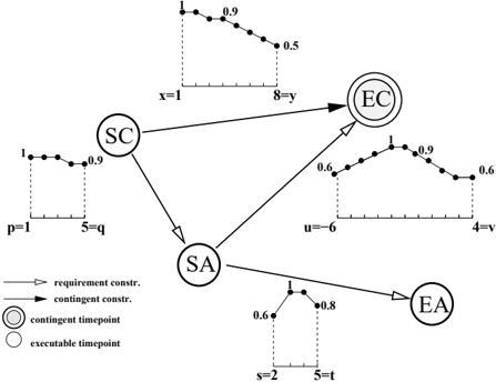
This scenario, rather tedious to describe in words, can be compactly represented by the STPPU shown in Figure 8 with the following features:

• a set of executable time-points SC (Start Clouds), SA (Start Aiming), EA (End Aiming);
• a contingent time-point EC (End Clouds);
• a set of soft requirement constraints on { SC → SA , SA → EC , SA → EA } ;
• a soft contingent constraint { SC → EC } ;

• the fuzzy semiring S FCSP = 〈 [0 , 1] , max , min , 0 , 1 〉 .

A solution of the STPPU in Figure 8 is the schedule s = { SC = 0 , SA = 2 , EC = 5 , EA = 7 } . The situation associated with s is the projection on the only contingent constraint, SC → EC , i.e. ω s = 5 , while the control sequence is the assignment to the executable time-points, i.e. δ s = { SC = 0 , SA = 2 , EA = 7 } . The global preference is obtained by considering the preferences associated with the projections on all constraints, that is pref(2) = 1 on SC → SA , pref(3) = 0 . 6 on SA → EC , pref(5) = 0 . 9 on SA → EA , and pref(5) = 0 . 8 on SC → EC . The preferences must then be combined using the multiplicative operator of the semiring, which is min , so the global preference of s is 0 . 6 . Another solution s ′ = { SC = 0 , SA = 4 , EC = 5 , EA = 9 } has global preference 0 . 8 . Thus s ′ is a better solution than s according to the semiring ordering since max(0 . 6 , 0 . 8) = 0 . 8 . /Box

4. Controllability with Preferences

We now consider how it is possible to extend the notion of controllability to accommodate preferences. In general we are interested in the ability of the agent to execute the time-points under its control, not only subject to all constraints but also in the best possible way with respect to preferences.

It transpires that the meaning of 'best possible way' depends on the types of controllability required. In particular, the concept of optimality must be reinterpreted due to the presence of uncontrollable events. In fact, the distinction on the nature of the events induces a difference on the meaning of the preferences expressed on them, as mentioned in the previous section. Once a scenario is given it will have a certain level of desirability, expressing how much the agent likes such a situation. Then, the agent often has several choices for the events he controls that are consistent with that scenario. Some of these choices might be preferable with respect to others. This is expressed by the preferences on the requirement constraints and such information should guide the agent in choosing the best possible actions to take. Thus, the concept of optimality is now 'relative' to the specific scenario. The final preference of a complete assignment is an overall value which combines how much the corresponding scenario is desirable for the agent and how well the agent has reacted in that scenario.

The concepts of controllability we will propose here are, thus, based on the possibility of the agent to execute the events under her control in the best possible way given the actual situation. Acting in an optimal way can be seen as not lowering further the preference given by the uncontrollable events.

4.1 Strong Controllability with Preferences

We start by considering the strongest notion of controllability. We extend this notion, taking into account preferences, in two ways, obtaining Optimal Strong Controllability and α -Strong Controllability , where α ∈ A is a preference level. As we will see, the first notion corresponds to a stronger requirement, since it assumes the existence of a fixed unique assignment for all the executable timepoints that is optimal in every projection. The second notion requires such a fixed assignment to be optimal only in those projections that have a maximum preference value not greater than α , and to yield a preference < α in all other cases.

/negationslash

Definition 21 (Optimal Strong Controllability) An STPPU P is Optimally Strongly Controllable (OSC) iff there is a viable execution strategy S s.t.

1. [ S ( P 1 )] x = [ S ( P 2 )] x , ∀ P 1 , P 2 ∈ Proj ( P ) and for every executable time-point x ;
2. S ( P ω ) ∈ OptSol ( P ω ) , ∀ P ω ∈ Proj ( P ) . /Box

In other words, an STPPU is OSC if there is a fixed control sequence that works in all possible situations and is optimal in each of them. In the definition, 'optimal' means that there is no other assignment the agent can choose for the executable time-points that could yield a higher preference in any situation. Since this is a powerful restriction, as mentioned before, we can instead look at just reaching a certain quality threshold:

Definition 22 ( α -Strong Controllability) An STPPU P is α -Strongly Controllable ( α -SC), with α ∈ A a preference, iff there is a viable strategy S s.t.

1. [ S ( P 1 )] x = [ S ( P 2 )] x , ∀ P 1 , P 2 ∈ Proj ( P ) and for every executable time-point x ;
2. S ( P ω ) ∈ OptSol ( P ω ) , ∀ P ω ∈ Proj ( P ) such that /negationslash ∃ s ′ ∈ OptSol ( P ω ) with pref ( s ′ ) > α ;

/negationslash

1. pref ( S ( P ω )) < α otherwise. /Box

In other words, an STPPU is α -SC if there is a fixed control sequence that works in all situations and results in optimal schedules for those situations where the optimal preference level of the projection is not > α in a schedule with preference not smaller than α in all other cases.

4.2 Weak Controllability with Preferences

Secondly, we extend similarly the least restrictive notion of controllability. Weak Controllability requires the existence of a solution in any possible situation, possibly a different one in each situation. We extend this definition by requiring the existence of an optimal solution in every situation.

Definition 23 (Optimal Weak Controllability) An STPPU P is Optimally Weakly Controllable (OWC) iff ∀ P ω ∈ Proj ( P ) there is a strategy S ω s.t. S ω ( P ω ) is an optimal solution of P ω . /Box

In other words, an STPPU is OWC if, for every situation, there is a control sequence that results in an optimal schedule for that situation.

Optimal Weak Controllability of an STPPU is equivalent to Weak Controllability of the corresponding STPU obtained by ignoring preferences, as we will formally prove in Section 6. The reason is that if a projection P ω has at least one solution then it must have an optimal solution. Moreover, any STPPU is such that its underlying STPU is either WC or not. Hence it does not make sense to define a notion of α -Weak Controllability.

4.3 Dynamic Controllability with Preferences

Dynamic Controllability (DC) addresses the ability of the agent to execute a schedule by choosing incrementally the values to be assigned to executable time-points, looking only at the past. When preferences are available, it is desirable that the agent acts not only in a way that is guaranteed to be consistent with any possible future outcome but also in a way that ensures the absence of regrets w.r.t. preferences.

Definition 24 (Optimal Dynamic Controllability) An STPPU P is Optimally Dynamically Controllable (ODC) iff there is a viable strategy S such that ∀ P 1 , P 2 ∈ Proj ( P ) and for any executable time-point x :

1. if [ S ( P 1 )] <x = [ S ( P 2 )] <x then [ S ( P 1 )] x = [ S ( P 2 )] x ;
2. S ( P 1 ) ∈ OptSol ( P 1 ) and S ( P 2 ) = OptSol ( P 2 ) . /Box

In other words, an STPPU is ODC if there exists a means of extending any current partial control sequence to a complete control sequence in the future in such a way that the resulting schedule will be optimal. As before, we also soften the optimality requirement to having a preference reaching a certain threshold.

Definition 25 ( α -Dynamic Controllability) An STPPU P is α -Dynamically Controllable ( α -DC) iff there is a viable strategy S such that ∀ P 1 , P 2 ∈ Proj ( P ) and for every executable time-point x :

1. if [ S ( P 1 )] <x = [ S ( P 2 )] <x then [ S ( P 1 )] x = [ S ( P 2 )] x ;
2. S ( P 1 ) ∈ OptSol ( P 1 ) and S ( P 2 ) ∈ OptSol ( P 2 ) if /negationslash ∃ s 1 ∈ OptSol ( P 1 ) with pref ( s 1 ) > α and /negationslash ∃ s 2 ∈ OptSol ( P 2 ) with pref ( s 2 ) > α ;

/negationslash

1. pref( S ( P 1 )) < α and pref( S ( P 2 )) < α otherwise. /Box

/negationslash

In other words, an STPPU is α -DC if there is a means of extending any current partial control sequence to a complete sequence; but optimality is guaranteed only for situations with preference > α . For all other projections the resulting dynamic schedule will have preference at not smaller than α .

4.4 Comparing the Controllability Notions

We will now consider the relation among the different notions of controllability for STPPUs.

Recall that for STPUs, SC = ⇒ DC = ⇒ WC (see Section 2). We start by giving a similar result that holds for the definitions of optimal controllability with preferences. Intuitively, if there is a single control sequence that will be optimal in all situations, then clearly it can be executed dynamically, just assigning the values in the control sequence when the current time reaches them. Moreover if, whatever the final situation will be, we know we can consistently assign values to executables, just looking at the past assignments, and never having to backtrack on preferences, then it is clear that every situation has at least an optimal solution.

Theorem 1 If an STPPU P is OSC, then it is ODC; if it is ODC, then it is OWC.

Proofs of theorems are given in the appendix. The opposite implications of Theorem 1 do not hold in general. It is in fact sufficient to recall that hard constraints are a special case of soft constraints and to use the known result for STPUs (Morris et al., 2001).

As examples consider the following two, both defined on the fuzzy semiring. Figure 9 shows an STPPU which is OWC but is not ODC. It is, in fact, easy to see that any assignment to A and C, which is a projection of the STPPU can be consistently extended to an assignment of B. However, we will show in Section 7 that the STPPU depicted is not ODC.

/negationslash

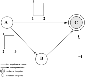
Figure 10, instead, shows an ODC STPPU which is not OSC. A and B are two executable timepoints and C is a contingent time-point. There are only two projections, say P 1 and P 2 , corresponding respectively to point 1 and point 2 in the AC interval. The optimal preference level for both is 1. In fact, 〈 A = 0 , C = 1 , B = 2 〉 is a solution of P 1 with preference 1 and 〈 A = 0 , C = 2 , B = 3 〉 is a solution of P 2 with preference 1. The STPPU is ODC. In fact, there is a dynamic strategy S that assigns to B value 2, if C occurs at 1, and value 3, if C occurs at 2 (assuming A is always assigned 0). However there is no single value for B that will be optimal in both scenarios.

Similar results apply in the case of α -controllability, as the following formal treatment shows.

Theorem 2 For any given preference level α , if an STPPU P is α -SC then it is α -DC.

Again, the converse does not hold in general. As an example consider again the STPPU shown in Figure 10 and α = 1 . Assuming α = 1 , such an STPPU is 1-DC but, as we have shown above, it is not 1 -SC.

Another useful result is that if a controllability property holds at a given preference level, say β , then it holds also ∀ α < β , as stated in the following theorem.

Theorem 3 Given an STPPU P and a preference level β , if P is β -SC (resp. β -DC), then it is α -SC (resp. α -DC), ∀ α < β .

Let us now consider case in which the preference set is totally ordered. If we eliminate the uncertainty in an STPPU, by regarding all contingent time-points as executables, we obtain an STPP. Such an STPP can be solved obtaining its optimal preference value opt . This preference level, opt , will be useful to relate optimal controllability to α -controllability. As stated in the following theorem, an STPPU is optimally strongly or dynamically controllable if and only if it satisfies the corresponding notion of α -controllability at α = opt .

Theorem 4 Given an STPPU P defined on a c-semiring with totally ordered preferences, let opt = max T ∈ Sol ( P ) pref ( T ) . Then, P is OSC (resp. ODC) iff it is opt -SC (resp. opt -DC).

For OWC, we will formally prove in Section 6 that an STPPU is OWC iff the STPU obtained by ignoring the preference functions is WC. As for the relation between α min -controllability and controllability without preferences, we recall that considering the elements of the intervals mapped in a preference ≥ α min coincides by definition to considering the underlying STPU obtained by ignoring the preference functions of the STPPU. Thus, α min -X holds iff X holds, where X is either SC or DC.

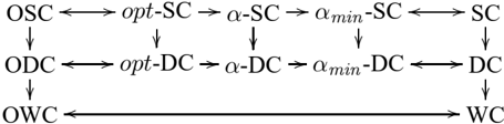
In Figure 11 we summarize the relationships holding among the various controllability notions when preferences are totally ordered. When instead they are partially ordered, the relationships opt -X and α min -X , where X is a controllability notion, do not make sense. In fact, in the partially ordered case, there can be several optimal elements and several minimal elements, not just one.

5. Determining Optimal Strong Controllability and α -Strong Controllability

In the next sections we give methods to determine which levels of controllability hold for an STPPU. Strong Controllability fits when off-line scheduling is allowed, in the sense that the fixed optimal control sequence is computed before execution begins. This approach is reasonable if the planning

/d15

/d15

/d15

/d15

/d15

/d15

/d111

/d111

/d47

/d47

Figure 11: Comparison of controllability notions for total orders. α min is the smallest preference over any constraint: opt ≥ α ≥ α min .

algorithm has no knowledge on the possible outcomes, other than the agent's preferences. Such a situation requires us to find a fixed way to execute controllable events that will be consistent with any possible outcome of the uncontrollables and that will give the best possible final preference.

5.1 Algorithm Best-SC

The algorithm described in this section checks whether an STPPU is OSC. If it is not OSC, the algorithm will detect this and will also return the highest preference level α such that the problem is α -SC.

All the algorithms we will present in this paper rely on the following tractability assumptions, inherited from STPPs: (1) the underlying semiring is the fuzzy semiring S FCSP defined in Section 2.2, (2) the preference functions are semi-convex, and (3) the set of preferences [0 , 1] is discretized in a finite number of elements according to a given granularity.

The algorithm Best-SC is based on a simple idea: for each preference level β , it finds all the control sequences that guarantee strong controllability for all projections such that their optimal preference is ≥ β , and optimality for those with optimal preference β . Then, it keeps only those control sequences that do the same for all preference levels > β .

The pseudocode is shown in Figure 12. The algorithm takes in input an STPPU P (line 1). As a first step, the lowest preference α min is computed. Notice that, to do this efficiently, the analytical structure of the preference functions (semi-convexity) can be exploited.

In line 3 the STPU obtained from P by cutting it at preference level α min is considered. Such STPU is obtained by applying function α min -Cut (STPPU G ) with G = P 5 . In general, the result of β -Cut ( P ) is the STPU Q β (i.e., a temporal problem with uncertainty but not preferences) defined as follows:

• Q β has the same variables with the same domains as in P;
• for every soft temporal constraint (requirement or contingent) in P on variables X i , and X j , say c = 〈 I, f 〉 , there is, in Q β , a simple temporal constraint on the same variables defined as { x ∈ I | f ( x ) ≥ β } .

Notice that the semi-convexity of the preference functions guarantees that the set { x ∈ I | f ( x ) ≥ β } forms an interval. The intervals in Q β contain all the durations of requirement and contingent events that have a local preference of at least β .

5. Notice that function β -Cut can be applied to both STPPs and STPPUs: in the first case the output is an STP, while in the latter case an STPU. Notice also that, α -Cut is a known concept in fuzzy literature.

/d111

/d111

/d111

/d111

/d47

/d47

/d47

/d47

/d15

/d15

/d47

/d47

/d47

/d47

/d15

/d15

/d47

/d47

/d47

/d47

/d15

/d15

/d111

/d111

/d111

/d111

/d47

/d47

/d47

/d47

/d15

/d15

Pseudocode for Best-SC 1. input STPPU P ; 2. compute α min ; 3. STPU Q α min ← α min -Cut ( P ); 4. if ( StronglyControllable ( Q α min ) inconsistent) write 'not α min -SC' and stop ; 5. else { 6. STP P α min ← StronglyControllable ( Q α min ); 7. preference β ← α min +1 ; 8. bool OSC ← false, bool α -SC ← false; 9. do { 10. STPU Q β ← β -Cut ( P ); 11. if ( PC ( Q β ) inconsistent) OSC ← true; 12. else { 13. if ( StronglyControllable ( PC ( Q β ) ) inconsistent) α -SC ← true; 14. else { 15. STP P β ← P β -1 ⊗ StronglyControllable ( PC ( Q β ) ) ; 16. if ( P β inconsistent) { α -SC ← true } ; 17. else { β ← β +1 } ; 18. } 19. } 20. } while (OSC=false and α -SC=false); 21. if (OSC=true) write 'P is OSC'; 22. if ( α -SC=true) write 'P is' ( β -1) '-SC'; 23. s e = Earliest-Solution( P β -1 ) , s l = Latest-Solution( P β -1 ) ; 24. return P β -1 , s e , s l ; 25. } ;

Once STPU Q α min is obtained, the algorithm checks if it is strongly controllable. If the STP obtained applying algorithm StronglyControllable (Vidal & Fargier, 1999) to STPU Q α min is not consistent, then, according to Theorem 3, there is no hope for any higher preference, and the algorithm can stop (line 4), reporting that the STPPU is not α -SC ∀ α ≥ 0 and thus is not OSC as well. If, instead, no inconsistency is found, Best-SC stores the resulting STP (lines 5-6) and proceeds moving to the next preference level α min +1 6 (line 7).

In the remaining part of the algorithm (lines 9-21), three steps are performed at each preference level considered:

• Cut STPPU P and obtain STPU Q β (line 10);
• Apply path consistency to Q β considering it as an STP: PC ( Q β ) (line 11);
• Apply strong controllability to STPU PC ( Q β ) (line 13).

Let us now consider the last two steps in detail.

Applying path consistency to STPU Q β means considering it as an STP, that is, treating contingent constraints as requirement constraints. We denote as algorithm PC any algorithm enforcing path-consistency on the temporal network (see Section 2.1 and Dechter et al., 1991). It returns the minimal network leaving in the intervals only values that are contained in at least one solution. This allows us to identify all the situations, ω , that correspond to contingent durations that locally have preference ≥ β and that are consistent with at least one control sequence of elements in Q β . In other words, applying path consistency to Q β leaves in the contingent intervals only durations that belong to situations such that the corresponding projections have optimal value at least β . If such a test gives an inconsistency, it means that the given STPU, seen as an STP, has no solution, and hence that all the projections corresponding to scenarios of STPPU P have optimal preference < β (line 11).

The third and last step applies StronglyControllable to path-consistent STPU PC ( Q β ), reintroducing the information on uncertainty on the contingent constraints. Recall that the algorithm rewrites all the contingent constraints in terms of constraints on only executable time-points. If the STPU is strongly controllable, StronglyControllable will leave in the requirement intervals only elements that identify control sequences that are consistent with any possible situation. In our case, applying StronglyControllable to PC ( Q β ) will find, if any, all the control sequences of PC ( Q β ) that are consistent with any possible situation in PC ( Q β ).

However, if STPU PC ( Q β ) is strongly controllable, some of the control sequences found might not be optimal for scenarios with optimal preference lower than β . In order to keep only those control sequences that guarantee optimal strong controllability for all preference levels up to β , the STP obtained by StronglyControllable ( PC ( Q β )) is intersected with the corresponding STP found in the previous step (at preference level β -1 ), that is P β -1 (line 15). We recall that given two two STPs, P 1 and P 2 , defined on the same set of variables, the STP P 3 = P 1 ⊗ P 2 has the same variables as P 1 and P 2 and each temporal constraint, c 3 ij = c 1 ij ⊗ c 2 ij , is the intersection of the corresponding intervals of P 1 and P 2 . If the intersection becomes empty on some constraint or the STP obtained is inconsistent, we can conclude that there is no control sequence that will guarantee strong controllability and optimality for preference level β and, at the same time, for all preferences

6. By writing α min +1 we mean the next preference level higher than α min defined in terms of the granularity of the preferences in the [0,1] interval.

Table 1: In this table each row corresponds to a preference level β and represents the intervals of STPU Q β obtained by cutting the STPPU in Figure 8 at level β .

STPU	( SC → EC )	( SC → SA )	( SA → EC )
Q 0 . 5 Q 0 . 6 Q 0 . 7 Q 0 . 8 Q 0 . 9 Q 1	[1 , 8] [1 , 7] [1 , 6] [1 , 5] [1 , 4] [1 , 2]	[1 , 5] [1 , 5] [1 , 5] [1 , 5] [1 , 5] [1 , 3]	[ - 6 , 4] [ - 6 , 4] [ - 5 , 2] [ - 4 , 1] [ - 3 , 0] [ - 2 , - 1]

Table 2: In this table each row corresponds to a preference level β and represents the intervals of STPU PC ( Q β ) obtained applying path consistency to the STPUs in Table 1.

STPU	( SC → EC )	( SC → SA )	( SA → EC )
PC ( Q 0 . 5 )	[1 , 8]	[1 , 5]	[ - 4 , 4]
PC ( Q 0 . 6 )	[1 , 7]	[1 , 5]	[ - 4 , 4]
PC ( Q 0 . 7 )	[1 , 6]	[1 , 5]	[ - 4 , 2]
PC ( Q 0 . 8 )	[1 , 5]	[1 , 5]	[ - 4 , 1]
PC ( Q 0 . 9 )	[1 , 4]	[1 , 5]	[ - 3 , 0]
PC ( Q 1 )	[1 , 2]	[2 , 3]	[ - 2 , - 1]

< β (line 16). If, instead, the STP obtained is consistent, algorithm Best-SC considers the next preference level, β +1 , and performs the three steps again.

The output of the algorithm is the STP, P β -1 , obtained in the iteration previous to the one causing the execution to stop (lines 23-24) and two of its solutions, s e and s l . This STP, as we will show shortly, contains all the control sequences that guarantee α -SC up to α = β -1 . Only if β -1 is the highest preference level at which cutting gives a consistent problem, then the STPPU is OSC. The solutions provided by the algorithm are respectively the the earliest, s e , and the latest, s l , solutions of P β -1 . In fact, as proved in (Dechter et al., 1991) and mentioned in Section 2.1, since P β -1 is minimal, the earliest (resp. latest) solution corresponds to assigning to each variable the lower (resp. upper) bound of the interval on the constraint defined on X 0 and the variable. This is indicated in the algorithm by procedures Earliest-Solution and Latest-Solution . Let us also recall that every other solution can be found from P β -1 without backtracking.

Before formally proving the correctness of algorithm Best-SC , we give an example.

Example 5 Consider the STPPU described in Example 4, and depicted in Figure 8. For simplicity we focus on the triangular sub-problem on variables SC , SA , and EC . In their example, α min = 0 . 5 . Table 1 shows the STPUs Q β obtained cutting the problem at each preference level β = 0 . 5 , . . . , 1 . Table 2 shows the result of applying path consistency (line 11) to each of the STPUs shown in Table 1. As can be seen, all of the STPUs are consistent. Finally, Table 3 shows the STPs defined only on executable variables, SC and SA , that are obtained applying StronglyControllable to the STPUs in Table 2.

Table 3: In this table each row corresponds to a preference level β and represents the intervals of STP StronglyControllable PC ( Q β ) obtained applying the strong controllability check to the STPUs in Table 2.

STP	( SC → SA )
StronglyControllable ( PC ( Q 0 . 5 ))	[4 , 5]
StronglyControllable ( PC ( Q 0 . 6 ))	[3 , 5]
StronglyControllable ( PC ( Q 0 . 7 ))	[4 , 5]
StronglyControllable ( PC ( Q 0 . 8 ))	[4 , 5]
StronglyControllable ( PC ( Q 0 . 9 ))	[4 , 4]
StronglyControllable ( PC ( Q 1 ))	[3 , 3]

By looking at Tables 2 and 3 it is easy to deduce that the Best-SC will stop at preference level 1. In fact, by looking more carefully at Table 3, we can see that STP P 0 . 9 consists of interval [4 , 4] on the constraint SC → SA , while StronglyControllable ( PC ( Q 1 )) consist of interval [3 , 3] on the same constraint. Obviously intersecting the two gives an inconsistency, causing the condition in line 16 of Figure 12 to be satisfied.

The conclusion of executing Best-SC on the example depicted in Figure8 is that it is 0 . 9 -SC but not OSC. Let us now see why this is correct. Without loss of generality we can assume that SC is assigned value 0. From the last line of Table 3 observe that the only value that can be assigned to SA that is optimal with both scenarios that have optimal preference 1 (that is when EC is assigned 1 or 2) is 3. However, assigning 3 to SA is not optimal if EC happens at 6, since this scenario has optimal preference value 0.7 (e.g. if SA is assigned 5) while in this case it would have a global preference 0.6 (given in constraint SA → EC ) 7 . /Box

5.2 Properties of Best-SC

We will now prove that algorithm Best-SC correctly identifies whether an STPPU P is OSC, and, if not, finds the highest preference level at which P is α -SC. Let us first consider the events in which Best-SC stops.

• Event 1. StronglyControllable ( Q α min ) is inconsistent (line 4);
• Event 2. PC ( Q γ ) returns an inconsistency (line 11);
• Event 3. PC ( Q γ ) is consistent but it is not strongly controllable (line 13);
• Event 4. PC ( Q γ ) is strongly controllable, however the intersection of the STP obtained by StronglyControllable ( PC ( Q γ ) ) with the STP obtained at the previous preference level, P γ -1 , is inconsistent (line 16).

First notice that the algorithm terminates.

Theorem 5 Given any STPPU P with a finite number of preference levels, the execution of algorithm Best-SC over P terminates.

7. Recall that in the fuzzy semiring context the global preference of any assignment is computed taking the minimum preference assigned to any of its projections.

Intuitively, either one of the termination events occur or all the preference levels will be exhausted.

Next, let us show that Best-DC is a sound and complete algorithm for checking if an STPPU is OSC and for finding the highest preference level at which it is α -SC.

As we have said before, cutting an STPPU P at a preference level γ gives an STPU Q γ . Moreover, every situation ω = { ω 1 , . . . , ω l } of Q γ can be seen as a situation of P such that f j ( ω j ) ≥ γ, ∀ j . This implies that every projection P ω ∈ Proj ( Q γ ) , which is an STP, corresponds to a projection P ω ∈ Proj ( P ) which is an STPP. For all situations ω of Q γ , in what follows we will write always P ω which should be interpreted as an STP when seen as a projection of Q γ and as an STPP when seen as a projection of P . In the following lemmas we state properties which relate the solutions of such projections in the two contexts: without and with preferences.

Theorem 6 Consider an STPPU P = 〈 N e , N c , L r , L c , S FCSP 〉 and preference level γ , and consider the STPU Q γ = 〈 N e , N c , L ′ r , L ′ c 〉 obtained by cutting P at γ , and STPU PC ( Q γ )= 〈 N e , N c , L ′′ r , L ′′ c 〉 . Then:

1. ∀ ω situation of P , P ω ∈ Proj ( PC ( Q γ )) iff opt P ( P ω ) ≥ γ ;
2. for every control sequence δ , δ is a solution of T γ = StronglyControllable ( PC ( Q γ ) , iff ∀ P ω ∈ Proj( PC ( Q γ )), T δ,ω ∈ Sol ( P ω ) and pref ( T δ,ω ) ≥ γ .

The first part of the theorem states that, by applying path consistency to STPU Q γ , we remove those situations that cannot be extended to complete solutions in Q γ , and thus correspond to projections having optimal preference strictly less than γ . The second part of the lemma considers the STP T γ obtained applying StronglyControllable after path consistency. In particular it is stated that all the solutions of T γ result, for all the projections of PC ( Q γ ), in solutions with preference at least γ . Notice that this implies that they result in optimal solutions for those projections of P having optimal preference exactly γ . They might not be optimal, however, for some projections with optimal preference strictly greater than γ .

From the above theorem, we get the following corollary, which clarifies the relation between the STPU obtained cutting an STPPU at preference level γ , and the γ -SC of the STPPU.

Corollary 1 Consider an STPPU P and a preference level γ and assume that ∃ ω , situation of P , such that opt ( P ω ) ≥ γ , where P ω is the corresponding projection. Then, if STPU PC ( Q γ ), obtained by cutting P at γ , and then applying path consistency, is not SC the P is not γ -SC.

Now if we consider all preference levels between α min and γ , and compute the corresponding STPs, say T α min , . . . , T γ , each such STP will identify the assignments to executable variables guaranteeing strong controllability and optimality at each level. By intersecting all these STPs we keep only the common solutions and thus those which guarantee strong controllability and optimality for all the situations of P with optimal preference smaller than or equal to γ .

Theorem 7 Consider an STPPU P , and all preference levels from α min to γ , and assume that the corresponding STPs, T α min , . . . , T γ obtained by cutting P at preference levels α min , . . . , γ , and enforcing strong controllability are consistent. Then, δ ∈ Sol ( P γ ) , where P γ = ⊗ i = α min ,...,γ T i , iff ∀ P ω ∈ Proj ( P ) : T δ,ω ∈ Sol ( P ω ) , if opt ( P ω ) ≤ γ , then pref ( T δ,ω ) = opt ( P ω ) , otherwise pref ( T δ,ω ) ≥ γ .

We now consider each of the events in which Best-SC can stop and for each of them we prove which of the strong controllability properties hold.

Theorem 8 If the execution of algorithm Best-SC on STPPU P stops due to the occurrence of Event 1 (line 4), then P is not α -SC ∀ α ≥ 0 .

This is the case when the underlying STPU obtained from the STPPU by ignoring the preference functions is not strongly controllable. Since cutting at higher preferences will give even smaller intervals there is no hope for controllability at any level and the execution can halt.

Theorem 9 If the execution of algorithm Best-SC on STPPU P stops due to the occurrence of Event 2 (line 11) at preference level γ , then

• γ -1 = opt = max T ∈ Sol ( P ) pref ( T ) ;
• P is OSC and a control sequence δ is a solution of STP P opt (returned by the algorithm) iff it is optimal in any scenario of P .

This event occurs when the algorithm cuts the STPPU at a given preference level and the STPU obtained, seen as an STP, is inconsistent. In particular, this means that no projection of Proj ( P ) has an optimal preference equal to or greater than this preference level. However, if such a level has been reached, then up to the previous level, assignments guaranteeing SC and optimality had been found. Moreover, this previous level must have been also the highest preference of any solution of P , opt ( P ) . This means that opt ( P ) -SC has been established, which by Theorem 4 is equivalent to OSC.

Theorem 10 If the execution of algorithm Best-SC on STPPU P stops due to the occurrence of Event 3 (line 13) or Event 4 (line 16) at preference level γ , then P is not OSC but it is ( γ -1) -SC and any solution δ of STP P γ -1 (returned by the algorithm) is such that, ∀ P ω ∈ Proj ( P ) : T δ,ω ∈ Sol ( P ω ) , if opt ( P ω ) ≤ γ -1 , then pref ( T δ,ω ) = opt ( P ω ) , otherwise pref ( T δ,ω ) ≥ γ -1 .

Intuitively, if the algorithm reaches γ and stops in line 13, then there are projections of P with optimal preference ≥ γ but the corresponding set of situations is not SC. Notice that this is exactly the situation considered in Corollary 1. If instead it stops in line 16, then this set of situations is SC, but none of the assignments guaranteeing SC for these situations does the same and is optimal for situations at all preference levels up to γ . In both cases the problem is not γ -SC. However, assuming that γ is the first level at which the execution is stopped the problem is γ -1 -SC.

We conclude this section considering the complexity of Best-SC .

Theorem 11 Determining the OSC or the highest preference level of α -SC of an STPPU with n variables and /lscript preference levels can be achieved in time O ( n 3 /lscript ) .

Notice that we cannot use a binary search over preference levels (in contrast to algorithms for STPPs), since the correctness of the procedure is based on the intersection of the result obtained at a given preference level, γ , with those obtained at all preference levels < γ .

The above theorem allows us to conclude that the cost of adding preferences, and thus a considerable expressive power, is low. In fact, the complexity is still polynomial and it has grown only of a factor equal to the number of preference levels.

6. Determining Optimal Weak Controllability

Optimal Weak Controllability is the least useful property in practice and also the property in which adding preferences has the smallest impact in terms of expressiveness. What OWC requires is the existence of an optimal solution in every possible scenario. This is equivalent to requiring the existence of a solution for every situation, as stated in the following theorem.

Theorem 12 STPPU P is OWC iff the STPU Q , obtained by simply ignoring the preference functions on all the constraints WC.

By ignoring the preference functions we mean mapping each soft constraint 〈 I, f 〉 into a hard constraint 〈 I 〉 defined on the same variables. This theorem allows us to conclude that, to check OWC, it is enough to apply algorithm WeaklyControllable as proposed in (Vidal & Ghallab, 1996) and described in Section 2. If, instead, we are given a scenario ω , then we can find an optimal solution of its projection, STPP Proj ( ω ) , by using one of the solvers described in (Rossi et al., 2002).

Let us now consider Example 4 again. Section 5 showed that the STPU obtained by cutting the STPPU of Figure 8 at preference level α min is strongly controllable. Since SC implies WC, we can conclude that the STPU is weakly controllable and, thus, that the STPPU in Figure 8 is Optimally Weakly Controllable.

7. Determining Optimal Dynamic Controllability and α -Dynamic Controllability

Optimal Dynamic Controllability (ODC) is the most interesting and useful property in practice. As described in Section 1, many industrial applications can only be solved in a dynamic fashion, making decisions in response to occurrences of events during the execution of the plan. This is true in the space application domains, where planning for a mission is handled by decomposing the problem into a set of scheduling subproblems, most of which depend on the occurrence of semipredictable, contingent events (Frank et al., 2001).

In this section we describe an algorithm that tests whether an STPPU P is ODC and, if not ODC, it finds the highest α at which P is α -DC. The algorithm presented bears some similarities with Best-SC , in the sense it decomposes the problem into STPUs corresponding to different preference levels and performs a bottom up search for dynamically controllable problems in this space.

Notice that the algorithm is attractive also in practice, since its output is the minimal form of the problem where only assignments belonging to at least one optimal solution are left in the domains of the executable time-points. This minimal form is to be given as input to an execution algorithm, which we also describe, that assigns feasible values to executable time-points dynamically while observing the current situation (i.e., the values of the contingent time-points that have occurred).

7.1 A Necessary and Sufficient Condition for Testing ODC

We now define a necessary and sufficient condition for ODC, which is defined on the intervals of the STPPU. We then propose an algorithm which tests such a condition, and we show that it is a sound and complete algorithm for testing ODC.

The first claim is that, given an STPPU, the dynamic controllability of the STPUs obtained by cutting the STPPU and applying PC at every preference level is a necessary but not sufficient condition for the optimal dynamic controllability of the given STPPU.

Theorem 13 Given an STPPU P , consider any preference level α such that STPU Q α , obtained cutting P at α , is consistent. If STPU PC ( Q α ) is not DC then P is not ODC and it is not β -DC, ∀ β ≥ α .

Unfortunately this condition is not sufficient, since an STPPU can still be not ODC even if at every preference level the STPU obtained after PC is DC. An example was shown in Figure 9 and is described below.

Example 6 Another potential application of STPPUs is scheduling for aircraft analysis of airborne particles (Coggiola, Shi, & Young, 2000). As an example consider an aircraft which is equipped with instruments as the Small Ice Detector and a Nevzorov probe, both of which are used to discriminate between liquid and ice in given types of clouds. Such analysis is important for the prediction of the evolution of precipitatory systems and of the occurrence and severity of aircraft icing (Field, Hogan, Brown, Illingworth, Choularton, Kaye, Hirst, & Greenaway, 2004). Both instruments need an uncertain amount of time to determine which is the predominant state, between liquid and ice, when activated inside a cloud.

In the example shown in Figure 9 we consider the sensing event represented by variables A and C and the start time of a maneuver of the aircraft represented by variable B . Due to how the instruments function, an aircraft maneuver can impact the analysis. In the example constraint AC represents the duration of the sensing event and the preference function models the fact that the earlier the predominant state is determined the better. Constraint AB models instead the fact that the maneuver should start as soon as possible, for example, due to time constraints imposed by the aircraft's fuel availability. Constraint BC models the fact that the maneuver should ideally start just before or just after the sensing event has ended.

Let us call P the STPPU depicted in Figure 9. In order to determine the highest preference level of any schedule of P we can, for example use algorithm Chop-solver (Rossi et al., 2002). The highest preference level at which cutting the functions gives a consistent STP is 1 (interval [3 , 3] on AB, [3 , 5] on AC and interval [0 , 2] on BC is a consistent STP). The optimal solutions of P , regarded as an STPP, will have global preference 1 .

Consider all the STPUs obtained by cutting at every preference level from the highest, 1, to the lowest 0.5. The minimum preference on any constraint in P is α min = 0 . 5 and, it is easy to see, that all the STPUs obtained by cutting P and applying PC at all preference levels from 0.5 to 1 are DC. However, P is not ODC. In fact, the only dynamic assignment to B that belongs to an optimal solution of projections corresponding to elements 3, 4 and 5 in [ x, y ] is 3. But executing B at 3 will cause an inconsistency if C happens at 10, since 10 -3 = 7 doesn't belong to [ u, v ] . /Box

We now elaborate on this example to find a sufficient condition for ODC. Consider the intervals on AB, [ p α , q α ] , and the waits < C,t α > obtained applying the DC checking algorithm at preference level α . These are shown in Table 4.

If we look at the first and last intervals, resp., at α = 1 and α = 0 . 5 , there is no way to assign a value to B that at the same time induces a preference 1 on constraints AB and BC, if C occurs at 3, 4 or 5, and that also satisfies the wait < C, 4 > , ensuring consistency if C occurs at 10. This depends on the fact that the intersection of [ p 1 , q 1 ] , i.e., [3] , and the sub interval of [ p 0 . 5 , q 0 . 5 ] that satisfies < C, 4 > , that is, [4 , 7] , is empty.

We claim that the non-emptiness of such an intersection, together with the DC of the STPUs obtained by cutting the problem at all preference levels is a necessary and sufficient condition for

Table 4: In this table each row corresponds to a preference level α and represents the corresponding interval and wait on the AB constraint of the STPPU shown in Figure 9.

α	[ p α , q α ]	wait
1	[3 , 3]
0 . 9	[3 , 4]	< C, 3 >
0 . 8	[3 , 5]	< C, 3 >
0 . 7	[3 , 6]	< C, 3 >
0 . 6	[3 , 7]	< C, 3 >
0 . 5	[3 , 7]	< C, 4 >

ODC. In the following section we will describe an algorithm which tests such a condition. Then, in Section 7.3, we will prove that such an algorithm is sound and complete w.r.t. testing ODC and finding the highest level of α -DC.

7.2 Algorithm Best-DC

The algorithm Best-DC echoes Section 5's algorithm for checking Optimal Strong Controllability. As done by Best-SC , it considers the STPUs obtained by cutting the STPPU at various preference levels. For each preference level, first it tests whether the STPU obtained considering it as an STP is path consistent. Then, it checks if the path consistent STPU obtained is dynamically controllable, using the algorithm proposed in (Morris et al., 2001). Thus, the control sequences that guarantee DC for scenarios having different optimal preferences are found. The next step is to select only those sequences that satisfy the DC requirement and are optimal at all preference levels.

The pseudocode is given in Figure 13. Algorithm Best-DC takes as input an STPPU P (line 1) and then computes the minimum preference, α min , assigned on any constraint (line 2).

Once α min is known, the STPU obtained by cutting P at α min is computed (line 3). This STPU can be seen as the STPPU P with the same variables and intervals on the constraints as P but with no preferences. Such an STPU, which is denoted as Q α min , is given as input to algorithm DynamicallyControllable . If Q α min is not dynamically controllable, then P is not ODC nor γ -DC (for any γ ≥ α min , hence for all γ ), as shown in Theorem 13. The algorithm detects the inconsistency and halts (line 4). If, instead, Q α min is dynamically controllable, then the STPU that is returned in output by DynamicallyControllable is saved and denoted with P α min (line 6). Notice that this STPU is minimal, in the sense that in the intervals there are only elements belonging to at least one dynamic schedule (Morris et al., 2001). In addition, since we have preferences, the elements of the requirement intervals, as well as belonging to at least one dynamic schedule, are part of optimal schedules for scenarios which have a projection with optimal preference equal to α min 8 .

In line 7 the preference level is updated to the next value in the ordering to be considered (according to the given preference granularity). In line 8 two Boolean flags, ODC and α -DC are defined. Setting flag ODC to true will signal that the algorithm has established that the problem is ODC, while setting flag α -DC to true will signal that the algorithm has found the highest preference level at which the STPPU is α -DC.

8. In fact, they all have preference at least α min by definition.

Pseudocode for Best-DC 1. input STPPU P ; 2. compute α min ; 3. STPU Q α min ← α min -Cut ( P ); 4. if ( DynamicallyControllable ( Q α min ) inconsistent) write 'not α min -DC' and stop ; 5. else { 6. STP P α min ← DynamicallyControllable ( Q α min ); 7. preference β ← α min +1 ; 8. bool ODC ← false, bool α -DC ← false; 9. do { 10. STPU Q β ← β -Cut ( P ); 11. if ( PC ( Q β ) inconsistent) ODC ← true; 12. else { 13. if ( DynamicallyControllable ( PC ( Q β ) ) inconsistent) α -DC ← true; 14. else { 15. STPU T β ← DynamicallyControllable ( PC ( Q β )); 16. if ( Merge ( P β -1 , T β ) FAILS) { α -DC ← true } 17. else { 18. STPU P β ← Merge ( P β -1 , T β ); 19. β ← β +1 ; 20. } ; 21. } ; 22. } ; 23. } while (ODC=false and α -DC=false); 24. if (ODC=true) write 'P is ODC'; 25. if ( α -DC=true) write 'P is' ( β -1) '-DC'; 26. return STPPU F β -1 ← resulting STPPU ( P , P β -1 ); 27. } ;

• Pseudocode for Merge 1. input (STPU T β , STPU T β +1 ); 2. STPU P β +1 ← T β ; 3. for each constraint AB, A and B executables, in P β +1 define interval [ p ′ , q ′ ] and wait t ′ , given { interval [ p β , q β ] , wait t β in T β } and { interval [ p β +1 , q β +1 ] , wait t β +1 in T β +1 } , as follows:; 4. if ( t β = p β and t β +1 = p β +1 ) (Precede - Precede) 5. p ′ ← max ( p β , p β +1 ) , q ′ ← min ( q β , q β +1 ) , t ′ ← max ( t β , t β +1 ) ; 6. if ( q ′ < p ′ ) return FAILED; 7. if ( p β < t β < q β and p β +1 ≤ t β +1 < q β +1 ) (Unordered - Unordered or Precede) 8. t ′ ← max ( t β , t β +1 ) , q ′ ← min ( q β , q β +1 ) ; 9. if ( q ′ < t ′ ) return FAILED; 10. output P β +1 .

Figure 14: Algorithm Merge .

Lines 9-25 contain the main loop of the algorithm. In short, each time the loop is executed, it cuts P at the current preference level and looks if the cutting has produced a path consistent STPU (seen as an STP). If so, it checks if the path consistent version of the STPU is also dynamically controllable and, if also this test is passed, then a new STPU is created by 'merging' the current results with those of previous levels.

We now describe each step in detail. Line 10 cuts P at the current preference level β . In line 11 the consistency of the STPU Q β is tested applying algorithm PC . If PC returns an inconsistency, then we can conclude that P has no schedule with preference β (or greater).

The next step is to check if STPU PC ( Q β ) is DC. Notice that this is required for all preference levels up to the optimal level in order for P to be ODC, and up to γ in order for P to be γ -DC (Theorem 13). If applying algorithm DynamicallyControllable detects that PC ( Q β ) is not dynamically controllable, then the algorithm sets flag α -DC to true. If, instead, PC ( Q β ) is dynamically controllable the resulting minimal STPU is saved and denoted T β (line 15).

In line 16, the output of procedure Merge is tested. This procedure is used to combine the results up to preference β -1 with those at preference β , by applying it to the STPU obtained at the end of the previous while iteration, P β -1 , and STPU T β . The pseudocode for Merge is shown in Figure 14, and we will describe it in detail shortly. If no inconsistency is found, the new STPU obtained by the merging procedure is denoted with P β (line 18) and a new preference level is considered (line 19).

Lines 24-27 take care of the output. Lines 24 and 25 will write in output if P is ODC or, if not, the highest γ at which it is γ -DC. In line 27 the final STPPU, F , to be given in output, is obtained from STPU P β -1 , that is, the STPU obtained by the last iteration of the while cycle which was completed with success (i.e., it had reached line 20). Function Resulting STPPU restores all the preferences on all the intervals of P β -1 by setting them as they are in P . We will show that the requirement constraints of F will contain only elements corresponding to dynamic schedules that are always optimal, if the result is that P is ODC, or are optimal for scenarios corresponding to projections with optimal preference ≤ γ and guarantee a global preference level of at least γ in all others, if the result is that P is γ -DC.

The pseudocode of procedure Merge is given in Figure 14. The input consists of two STPUs defined on the same set of variables. In describing how Merge works, we will assume it is given in input two STPUs, T β and T β +1 , obtained by cutting two STPPUs at preference levels β and β +1 and applying, by hypothesis with success, PC and DynamicallyControllable (line 1 Figure 14).

In line 2, Merge initializes the STPU which will be given in output to T β . As will be formally proven in Theorem 14, due to the semi-convexity of the preference functions we have that Proj ( T β +1 ) ⊆ Proj ( T β ) . Notice that Merge leaves all contingent constraints unaltered. Thus, all the projection with optimal preference β or β +1 are contained in the set of projections of P β +1 .

Merge considers every requirement constraint defined on any two executables, say A and B, respectively in T β and T β +1 . Since we are assuming that algorithm DynamicallyControllable has been applied to both STPUs, there can be some waits on the intervals. Figure 6 illustrates the three cases in which the interval on AB can be. If the wait expires after the upper bound of the interval (Figure 6 (a)), then the execution of B must follow the execution of every contingent time-point ( Follow case ). If the wait coincides with the lower bound of the interval (Figure 6 (b)), then the execution of B must precede that of any contingent time-point ( Precede case ). Finally, as shown in Figure 6 (c), if the wait is within the interval, then B is in the Unordered case with at least a contingent time-point, say C.

Merge considers in which case the corresponding intervals are in T β and in T β +1 (line 3). Such intervals are respectively indicated as [ p β , q β ] , with wait t β , and [ p β +1 , q β +1 ] , with wait t β +1 . Merge obtains a new interval [ p ′ , q ′ ] and new wait t ′ , which will replace the old wait in T β +1 . Interval [ p ′ q ′ ] will contain all and only the values which are projections on the AB constraint of some optimal solution of some STPP corresponding to a situation in T β or T β +1 . Wait t ′ is the wait that should be respected during a dynamic execution in order to guarantee that the solution obtained is optimal, if the projection corresponding to the final scenario has preference β or β +1 .

Due to the semi-convexity of the preference functions it cannot be the case that:

• AB is a Follow or a Precede case in T β and an Unordered case in T β +1 ;
• AB is a Follow case in T β and a Precede case in T β +1 ;
• AB is a Precede case in T β and a Follow case in T β +1 ;

This means that the cases which should be considered are:

• AB is a Follow case in both T β and T β +1 ;
• AB is a Precede case in T β and in T β +1 ;
• AB is a Unordered case in T β and a Precede or an Unordered case in T β +1 ;

In the first two cases the AB interval is left as it is in T β +1 . A formal motivation of this is contained in the proof of Theorem 14. However, informally, we can say that the AB interval in T β +1 already satisfies the desired property.

In lines 4 and 5 the case in which AB is in a Precede case in both STPUs is examined. Here, B will always occur before any contingent time-point. The values in the [ p β , q β ] (resp. [ p β +1 , q β +1 ] ) are assignments for B that will be consistent with any future occurrence of C mapped into a preference ≥ β (resp. ≥ β + 1 ). Clearly the intersection should be taken in order not to lower the

preference if C occurs with preference ≥ β +1 . Line 6 considers the event in which such intersection is empty. This means that there is no common assignment to B, given that of A, that will be optimal both in scenarios with optimal preference β and in scenarios with optimal preference β +1 .

In lines 7 and 8 two scenarios are considered: when AB is in the Unordered case in T β and in the Precede case in T β +1 and when AB is in the Unordered case in both STPUs. Figure 15 shows the second case. Merge takes the union of the parts of the intervals preceding the wait and the intersection of the parts following the wait. The intuition underlying this is that any execution of B identifying an element of either [ p β , t β [ or [ p β +1 , t β +1 [ will be preceded by the execution of all the contingent time-points for which it has to wait. This means that when B is executed, for any such contingent time-point C, both the time at which C has been executed, say t C , and the associated preference, say f AC ( t C ) , on constraint AC in STPPU P will be known. The propagation of this information will allow us to identify those elements of [ p β , t β [ (resp. [ p β +1 , t β +1 [ ) that have a preference ≥ f AC ( t C ) and thus an optimal assignment for B. This means that all the elements in both interval [ p β , t β [ and interval [ p β +1 , t β +1 [ are eligible to be chosen. For example, if f AC ( t C ) = β there might be values for B with preference equal to β that are optimal in this case but would not if C occurred at a time such that f AC ( t C ) > β . But since in any case we know when and with what preference C has occurred, it will be the propagation step that will prune non-optimal choices for B. In short, leaving all elements allows more flexibility in the propagation step. Moreover, as will be proven in Theorem 14, p β ≤ p β +1 .

If instead we consider elements of interval [ t β , q β ] , we know that they identify assignments for B that can be executed regardless of when C will happen (however we know it will happen with a preference greater ≥ β ). This means that we must take the intersection of this part with the corresponding one, [ t β +1 , q β +1 ] , in order to guarantee consistency and optimality also when C occurs at any time with preference = β + 1 . An easy way to see this is that interval [ t β , q β ] may contain elements that in P are mapped into preference β . These elements can be optimal in scenarios in which C happens at a time associated with a preference = β in the AC constraint; however, they cannot be optimal in scenarios with C occurring at a time with preference β +1 .

Line 9 handles the case in which the two parts of the intervals, following the waits, have an empty intersection. In this case, optimality cannot be guaranteed neither at level β nor β + 1 , in particular if the contingent events occur after the waits expire.

7.3 Properties of Best-DC

Wewill now show that Best-DC is a sound and complete algorithm for testing ODC and for finding the highest preference level at which the STPPU given in input is α -DC. We recall, once more, that all the results that follow rely on the tractability assumptions requiring semi-convex preference functions and the fuzzy semiring 〈 [0 , 1] , max, min, 0 , 1 〉 as underlying structure.

Let us consider STPPU P and STPUs T β and T β +1 , as defined in the previous section. Then, STPU P β +1 = Merge ( T β , T β +1 ) will have the same contingent constraints as T β 9 and requirement constraints as defined by the merging procedure. We start by proving that Merge is a sound and complete algorithm for testing the existence of a viable dynamic strategy, common to both such STPUs, which is optimal for projections having optimal preference equal to either β or β +1 .

9. We recall that the projections of T β coincide with the projections of STPPU P with optimal preference ≥ β (see Theorem 6), and that, due to the semi-convexity of the preference functions, Proj ( T β +1 ) ⊆ Proj ( T β ) .

Theorem 14 Consider STPPU P and STPUs, T β and T β +1 , obtained by cutting P respectively at level β and β +1 and applying PC , without finding inconsistencies, and DynamicallyControllable with success. Consider STPU P β +1 = Merge ( T β , T β +1 ).

Then, Merge ( T β , T β +1 ) does not fail if and only if

• P β +1 is dynamically controllable and
• there is a viable dynamic strategy S such that for every projection P i ∈ Proj ( P β +1 ) ,
• -if opt ( P i ) = β or opt ( P i ) = β +1 in P , pref ( S ( P i )) = opt ( P i ) ;
• -otherwise pref ( S ( P i )) ≥ β +1 .

The following theorem extends the result for the merging procedure to more than two preference levels, in particular to all preference levels smaller or equal to a given threshold β .

Theorem 15 Consider STPPU P and for every preference level, α , define T α as the STPU obtained by cutting P at α , then applying PC and then DynamicallyControllable . Assume that ∀ α ≤ β , T α is DC. Consider STPU P β :

with α min the minimum preference on any constraint in P. Assume that, when applied, Merge always returned a consistent STPU. Then, there is a viable dynamic strategy S , such that ∀ P i ∈ Proj ( P ) , if opt ( P i ) ≤ β then S ( P i ) is an optimal solution of P i , otherwise pref ( S ( P i )) ≥ β +1 .

Theorem 15 allows us to prove the main result. Informally, Best-DC applies Merge from the lowest preference to the highest threshold γ , above which the returned problem becomes inconsistent. If there is no projection of the STPPU with an optimal solution higher than γ , then, by using Theorem 15, we can conclude that the STPPU is ODC; otherwise it is γ -DC.

Let us start by enumerating the conditions at which Best-DC terminates:

• Event 1. Best-DC stops because the STPU obtained at level α min is not DC (line 4);
• Event 2. Best-DC exits because it has reached a preference level β at which the STPU (seen as an STP) is not path consistent (line 11);
• Event 3. Best-DC stops because it has reached a preference level β at which the path consistent STPU is not dynamically controllable (line 13);
• Event 4. Best-DC stops because procedure Merge has found an inconsistency (line 16).

The following theorem shows that the execution of Best-DC always terminates.

Theorem 16 Given an STPPU P, the execution of algorithm Best-DC on P terminates.

Best-DC considers each preference level, starting from the lowest and moving up each time of one level according to the granularity of the preference set. It stops either when an inconsistency is found or when all levels, which are assumed to be finite, have been precessed.

We are now ready to prove the soundness and completeness of Best-DC . We split the proof into three theorems, each considering a different terminating condition. The first theorem considers the case in which the underlying STPU obtained from P , by ignoring the preferences, is not DC. In such a case the output is that the STPPU is not α -DC at any level and thus is not ODC.

Theorem 17 Given an STPPU P as input, Best-DC terminates in line 4 iff /negationslash ∃ α ≥ 0 such that P is α -DC.

The next theorem considers the case in which the highest preference level reached with success by the merging procedure is also the highest optimal preference of any projection of P . In such a case, the problem is ODC.

Theorem 18 Given an STPPU P as input, Best-DC terminates in line 11 iff P is ODC.

The last result considers the case in which there is at least a projection with an optimal preference strictly higher than the highest reached with success by the merging procedure. In such case the problem is not ODC and Best-DC has found the highest level at which the STPPU α -DC.

Theorem 19 Given STPPU P in input, Best-DC stops at lines 13 or 16 at preference level β iff P is ( β -1) -DC and not ODC.

As mentioned in Section 2.3, in (Morris & Muscettola, 2005), it is proven that checking DC of an STPU can be done in O ( n 5 ) , where n is the number of variables. The revised algorithm processes the distance graph of the STPU, rather than its constraint graph. It also maintains additional information, in the form of additional labeled edges which correspond to waits. The main feature of the new algorithm, as noted earlier, it is a strongly polynomial algorithm for determining the dynamic controllability of an STPU. What is important in our context is to stress the fact that the output of the two algorithms, presented in (Morris et al., 2001) and (Morris & Muscettola, 2005), is essentially the same. In fact it is easy to obtain, in polynomial time O ( n 2 ) , the constraint graph with waits produced by DynamicallyControllable starting from the distance graph produced by the new algorithm, and vice versa.

Theorem 20 The complexity of determining ODC or the highest preference level α of α -DC of an STPPU with n variables, a bounded number of preference levels /lscript is time O ( n 5 /lscript ) .

The complexity result given in Theorem 20 is unexpectedly good. In fact, it shows that the cost of adding a considerable expressive power through preferences to STPUs is a factor equal to the number of different preference levels. This implies that solving the optimization problem and, at the same time, the controllability problem, remains in P, if the number of different preference levels is bounded.

7.4 The Execution Algorithm

The execution algorithm we propose is very similar to that for STPUs presented in (Morris et al., 2001), which we described in Section 2 and shown in Figure 7. Of course the execution algorithm for STPPUs will take in input an STPPU to which Best-DC has been successfully applied. In line 2 of Figure 7, the algorithm performs the initial propagation from the starting point. The main difference between our STPPU execution algorithm and the STPU algorithm in (Morris et al., 2001) is that the definition of 'propagation' also involves preferences.

Definition 26 (soft temporal propagation) Consider an STPPU P and a variable Y ∈ P and a value v Y ∈ D ( Y ) . Then propagating the assignment Y = v Y in P , means:

• for all constraints, c XY involving Y such that X is already assigned value v X ∈ D ( X ) : replace the interval on c XY with interval 〈 [ v Y -v X , v Y -v X ] 〉 ;
• cut P at preference level min X { f c XY ( v Y -v X ) } . /Box

We will call ODC-Execute the algorithm DC-Execute where propagation is defined as in Definition 26. Assume we apply ODC-Execute to an ODC or α -DC STPPU P to which Best-DC has been applied. If, up to a given time T , the preference of the partial schedule was β , then we know that if P was ODC or α -DC with α ≥ β , by Theorem 14 and Theorem 15, the execution algorithm has been assigning values in T β +1 . Assume now that a contingent event occurs and lowers the preference to β -2 . This will be propagated and the STPPU will be cut at preference level β -2 . From now on, the execution algorithm will assign values in T β -2 and, by Theorem 14 and Theorem 15, the new waits imposed will be such that the assignments for the executables will be optimal in any situation where the optimal preference is ≤ β -2 . In all other situations such assignments guarantee a preference of at least β -2 .

8. Using the Algorithms

Section 4.4 described the relations between our notions of controllability. As a general strategy, given an STPPU, the first property to consider is OSC. If it holds, the solution obtained is feasible and optimal in all possible scenarios. However, OSC is a strong property and holds infrequently. If the STPPU is not OSC, but we still need to have a control sequence before execution begins, Best-SC will find the best solution that is consistent with all possible future situations.

Most commonly, dynamic controllability will be more useful. If the control sequence needs not be known before execution begins, ODC is ideal. Notice that, from the results in Section 4.4, an STPPU may be not OSC and still be ODC. If, however, the STPPU is not even ODC, then

Best-DC will give a dynamic solution with the highest preference. Recall, as we have shown in Section 4.4, that for any given preference level α , α -SC implies α -DC but not vice versa. Thus, it may be that a given STPPU is β -SC and γ -DC with γ > β . Being β -SC means that there is a fixed way to assign values to the executables such that it will be optimal only in situations with optimal preference ≤ β and will give a preference at least β in all other cases. On the other hand, γ -DC implies that a solution obtained dynamically, by the ODC-Execute algorithm, will be optimal for all those situations where the best solution has preference ≤ γ and will yield a preference ≥ γ in all other cases. Thus, if γ > β , using the dynamic strategy will guarantee optimality in more situations and a higher preference in all others.

The last possibility is to check OWC. This will at least allow the executing agent to know in advance if there is some situation that has no solution. Moreover, if the situation is revealed just before the execution begins, using any of the solvers for STPPs described in (Rossi et al., 2002) will allow us to find an optimal assignment for that scenario.

9. Related Work

In this section we survey work which we regard as closely related to ours. Temporal uncertainty has been studied before, but it has been defined in different ways according to the different contexts where it has been used.

We start considering the work proposed by Vila and Godo (1994). They propose Fuzzy Temporal Constraint Networks , which are STPs where the interval in each constraint is mapped into a possibility distribution. In fact, they handle temporal uncertainty using possibility theory (Zadeh, 1975), using the term 'uncertainty' to describe vagueness in the temporal information available. Their aim is to model statements as 'He called me more or less an hour ago', where the uncertainty is the lack of precise information on a temporal event. Their goal thus is completely different from ours. In fact, we are in a scenario where an agent must execute some activities at certain times, and such activities are constrained by temporal relations with uncertain events. Our goal is to find a way to execute what is in the agents control in a way that will be consistent whatever nature decides in the future.

In (Vila & Godo, 1994), instead, they assume to have imprecise temporal information on events happened in the past. Their aim is to check if such information is consistent, that is, if there are no contradictions implied and to study what is entailed by the set of constraints. In order to model such imprecise knowledge, possibilities are again used. Every element of an interval is mapped into a value that indicates how possible that event is or how certain it is. Thus, another major difference with their approach is that they do not consider preferences, only possibilities. On the other hand, in the work presented here we do not allow to express information on how possible or probable a value is for a contingent time-point. This is one of the lines of research we want to pursue in the future. Moreover, in (Vila & Godo, 1994), they are concerned with the classical notion of consistency (consistency level) rather than with controllability.

Another work related to the way we handle uncertainty is that of Badaloni and Giacomin (2000). They introduce Flexible Temporal Constraints where soft constraints are used to express preferences among feasible solutions and prioritized constraints are used to express the degree of necessity of the constraints' satisfaction. In particular, they consider qualitative Allen-style temporal relations and they associate each such relation to a preference. The uncertainty they deal with is not on the time of occurrence of an event but is on whether a constraint belongs or not to the constraint problem.

In their model, information coming from plausibility and information coming from preferences is mixed and is not distinguishable by the solver. In other words, it is not possible to say whether a solution is bad due to its poor preference on some relation or due to it violating a constraint with a high priority. In our approach, instead, uncertainty and preferences are separated. The compatibility with an uncertain event does not change the preference of an assignment to an executable. The robustness to temporal uncertainty is handled intrinsically by the different degrees of controllability.

In (Dubois, HadjAli, & Prade, 2003b) the authors consider fuzziness and uncertainty in temporal reasoning by introducing Fuzzy Allen Relations . More precisely, they present an extension of Allen relational calculus, based on fuzzy comparators expressing linguistic tolerance. Dubois et al. (2003b) want to handle situations in which the information about dates and relative positions of intervals is complete but, for some reason, there is no interest in describing it in a precise manner. For example, when one wants to speak only in terms of 'approximate equality', or proximity rather that in terms of precise equality. Secondly, they want to be able to deal with available information pervaded with imprecision, vagueness or uncertainty. In the framework we have presented we restrict the uncertainty to when an event will occur within a range. On the other hand, we put ourselves into a 'complete ignorance' position, that would be equivalent, in the context of (Dubois et al., 2003b), to setting to 1 all possibilities of all contingent events. Moreover, in (Dubois et al., 2003b) they do not allow preferences nor address controllability. Instead, they consider, similarly to (Vila & Godo, 1994), the notions of consistency and entailment. The first notion is checked by computing the transitive closure of the fuzzy temporal relations using inference rules appropriately defined. The second notion is checked by defining several patterns of inference.

Another work which addresses also temporal uncertainty is presented in (Dubois, Fargier, & Prade, 1995) and in (Dubois, Fargier, & Prade, 2003a). In this work both preferences and activities with ill-known durations in the classical job-shop scheduling problem are handled using the fuzzy framework. There are three types of constraints: precedence constraints, capacity constraints and due dates, and release time constraints. In order to model such unpredictable events they use possibility theory. As the authors mention in (Dubois et al., 1995), possibility distributions can be viewed as modeling uncertainty as well as preference (see Dubois, Fargier, & Prade, 1993). Everything depends on whether the variable X on which the possibility distribution is defined is controllable or not. Thus Dubois et al. (1995) distinguish between controllable and uncontrollable variables. However they do not allow to specify preferences on uncontrollable events. Our preference functions over contingent constraints would be interpreted as possibility distributions in their framework. In some sense, our work is complementary to theirs. We assume a constraint possibility distribution on contingent events always equal to 1 and we allow no representation of any further information on more or less possible values; on the other hand, we allow to specify preferences also on uncontrollable events. They, on the contrary, allow to put possibility distributions on contingent events, but not preferences.

Finally, Dubois et al. (1995) show that a scheduling problem with uncertain durations can be formally expressed by the same kind of constraints as a problem involving what they call flexible durations (i.e. durations with fuzzy preferences). However the interpretation is quite different: in the case of flexible durations, the fuzzy information comes from the specifications of preferences and represents the possible values that can be assigned to a variable representing a duration. In the case of imprecisely known durations, the fuzzy information comes from uncertainty about the real value of some durations. The formal correspondence between the two constraints is so close that the authors do not distinguish among them when describing the solving procedure. Further, the problem

they solve is to find the starting times of activities such that these activities take place within the global feasibility window whatever the actual values of the unpredictable durations will be . Clearly this is equivalent to Optimal Strong Controllability. They do not address the problem of dynamic or weak controllability with preferences.

10. Summary and Future Work

We have defined a formalism to model problems with quantitative temporal constraints with both preferences and uncertainty, and we have generalized to this formalism three classical notions of controllability (that is, strong, weak and dynamic). We have then focused on a tractable class of such problems, and we have developed algorithms that check the presence of these properties.

This work advances the state of the art in temporal reasoning and uncertainty since it provides a way to handle preferences in this context, and to select the best solution (rather than a feasible one) in the presence of uncontrollable events. Moreover, it shows that the computational properties of the controllability checking algorithms do not change by adding preferences. In particular, dynamic controllability can still be checked in polynomial time for the considered class of problems, producing dynamically temporal plans under uncertainty that are optimal with respect to preferences.

Among the future directions we want to pursue within this line of research, the first is a deeper study of methods and algorithms for adding preferences different from fuzzy ones. Notice that the framework that we have proposed here is able to represent any kind on preference within the soft constraint framework. However, our algorithms apply only to fuzzy preferences and semiconvex functions. In particular, we would like to consider the impact on the design and complexity of algorithms when there are uncontrollable events and the underlying preference structures is the weighted or the probabilistic semiring. Both of these semirings are characterized by non-idempotent multiplicative operators. This can be a problem when applying constraint propagation (Bistarelli et al., 1997), such as path-consistency, in such constraints. Thus search and propagation techniques will have to be adapted to an environment featuring uncertainty as well. It should be noticed that in (Peintner & Pollack, 2005) some algorithms for finding optimal solutions of STPs with preferences in the weighted semiring have been proposed. Another interesting class of preferences are utilitarian ones. In such a context each preference represents a utility and the goal is to maximize the sum of the utilities. Such preferences have been used in a temporal context without uncertainty for example in (Morris, Morris, Khatib, Ramakrishnan, & Bachmann, 2004).

Recently, another approach for handling temporal uncertainty has been introduced in (Tsamardinos, 2002; Tsamardinos, Pollack, & Ramakrishnan, 2003a): Probabilistic Simple Temporal Problems (PSTPs); similar ideas are presented in (Lau, Ou, & Sim, 2005). In the PSTP framework, rather than bounding the occurrence of an uncontrollable event within an interval, as in STPUs, a probability distribution describing when the event is more likely to occur is defined on the entire set of reals. As in STPUs, the way the problem is solved depends on the assumptions made regarding the knowledge about the uncontrollable variables. In particular they define the Static Scheduling Optimization Problem , which is the equivalent to finding an execution satisfying SC in STPUs, and the Dynamic Scheduling Optimization Problem , equivalent to finding a dynamic execution strategy in the context of STPUs. In the above framework, optimal means 'with the highest probability of satisfying all the constraints'. Preferences are not considered in this framework. We believe it would be interesting to add preferences also to this approach. A first step could consists of keeping, for each strategy, separately its global preference and its probability of success. In this way we

could use the existing frameworks for handling the two aspects. Then, we can order the strategies by giving priority to preferences, thus taking in some sense a risky attitude, or, on the contrary, by giving priority to probabilities, adopting a more cautious attitude. A step in this direction has been recently proposed in (Morris, Morris, Khatib, & Yorke-Smith, 2005), where, however, the authors, rather than actually extending the notions of consistency of PSTPs to handle preferences, consider inducing preferences from probabilities. In contrast, our approach is preliminary advanced in (Pini, Rossi, & Venable, 2005).

Up to now we have focused our attention on non-disjunctive temporal problems, that is, with only one interval per constraint. We would like to consider adding uncertainty to Disjunctive Temporal Problems (Stergiou & Koubarakis, 2000), and to consider scenarios where there are both preferences and uncertainty. Such problems are not polynomial even without preferences or uncertainty but it has been shown that the cost of adding preferences is small (Peintner & Pollack, 2004), so we hope that the same will hold in environments with uncertainty as well. Surprisingly, uncertainty in Disjoint Temporal Problems has not been considered yet, although it is easy to see how allowing multiple intervals on a constraint is itself a form of uncontrollability. We, thus, plan to start defining DTPUs (preliminary results are in Venable and Yorke-Smith, 2005) and then to merge this approach with the existing one for DTPPs.

Extending Conditional Temporal Problems , a framework proposed in (Tsamardinos, Vidal, & Pollack, 2003b), is also a topic of interest for us. In such model a Boolean formula is attached to each temporal variable. These formulae represent the conditions which must be satisfied in order for the execution of events to be enabled. In this framework the uncertainty is on which temporal variables will be executed. We believe that it would be interesting to extend this approach in order to allow for conditional preferences: allowing preference functions on constraints to have different shapes according to the truth values of some formulas, or the occurrence of some event at some time. This would provide an additional gain in expressiveness, allowing one to express the dynamic aspect of preferences that change over time.

Appendix A

Theorem 1 If an STPPU P is OSC, then it is ODC; if it is ODC, then it is OWC.

Proof: Let us assume that P is OSC. Then there is a viable execution strategy S such that, ∀ P 1 , P 2 ∈ Proj ( P ) and for every executable time-point x , [ S ( P 1 )] x = [ S ( P 2 )] x and S ( P 1 ) ∈ OptSol ( P 1 ) and S ( P 2 ) ∈ OptSol ( P 2 ) . Thus, in particular, [ S ( P 1 )] x = [ S ( P 2 )] x for every pair f projections such that [ S ( P 1 )] <x = [ S ( P 2 )] <x . This allows us to conclude that if P is OSC then it is also ODC and any strategy which is a witness of OSC is also a witness of ODC.

Let us now assume that P is ODC. Then, in particular, there is a viable dynamic strategy S such that ∀ P 1 ∈ Proj ( P ) , S ( P 1 ) is an optimal solution of P 1 . This clearly means that every projection has at least an optimal solution. Thus P is OWC. /Box

Theorem 2 For any given preference level α , if an STPPU P is α -SC then it is α -DC.

/negationslash

Proof: Assume that P is α -SC. Then there is a viable strategy S such that: [ S ( P 1 )] x = [ S ( P 2 )] x , ∀ P 1 , P 2 ∈ Proj ( P ) and for every executable time-point x , and S ( P ω ) is an optimal solution of projection P ω , if there is no optimal solution of P ω with preference > α and pref ( S ( P ω )) < α , otherwise.

Thus, [ S ( P 1 )] x = [ S ( P 2 )] x also for all pairs of projections, P 1 and P 2 such that [ S ( P 1 )] <x = [ S ( P 2 )] <x . This implies that P is α -DC. /Box

Theorem 3 Given an STPPU P and a preference level β , if P is β -SC (resp. β -DC), then it is α -SC (resp. α -DC), ∀ α < β .

/negationslash

Proof: If P is β -SC then there is a viable strategy S such that: [ S ( P 1 )] x = [ S ( P 2 )] x , ∀ P 1 , P 2 ∈ Proj ( P ) and for every executable time-point x , and S ( P ω ) is an optimal solution of P ω if there is no optimal solution of P ω with preference > β and pref ( S ( P ω )) < β , otherwise. But, of course, ∀ α < β the set of projections with no optimal solution with preference > α is included in that of projections with no optimal solution with preference > β . Moreover, for all the other projections, P z , pref ( S ( P z )) < β implies that pref ( S ( P z )) < α since β > α . Similarly for β -DC. /Box

/negationslash

/negationslash

Theorem 4 Given an STPPU P , let opt = max T ∈ Sol ( P ) pref ( T ) . Then, P is OSC (resp. ODC) iff it is opt -SC (resp. opt -DC).

Proof: The result comes directly from the fact that ∀ P i ∈ Proj ( P ) , opt ( P i ) ≤ opt , and there is always at least a projection, P j , such that opt ( P j ) = opt . /Box

Theorem 5 Given any STPPU P with a finite number of preference levels, the execution of algorithm Best-SC over P terminates.

Proof: Consider STPPU P and its optimal preference value opt = max T ∈ Sol ( P ) pref ( T ) , that is, the highest preference assigned to any of its solutions. By definition, Q opt +1 is not consistent. This means that if the algorithm reaches level opt +1 (that is, the next preference level higher than opt in the granularity of the preferences) then the condition in line 11 will be satisfied and the execution will halt. By looking at lines 9-20 we can see that either one of the events that cause the execution to terminate occurs or the preference level is incremented in line 16. Since there is a finite number of preference levels, this allows us to conclude that the algorithm will terminate in a finite number of steps. /Box

Theorem 6 Consider an STPPU P = 〈 N e , N c , L r , L c , S FCSP 〉 and preference level γ , and consider the STPU Q γ = 〈 N e , N c , L ′ r , L ′ c 〉 obtained by cutting P at γ , and STPU PC ( Q γ )= 〈 N e , N c , L ′′ r , L ′′ c 〉 . Then:

1. ∀ ω situation of P , P ω ∈ Proj ( PC ( Q γ )) iff opt P ( P ω ) ≥ γ ;
2. for every control sequence δ , δ is a solution of T γ = StronglyControllable ( PC ( Q γ ) iff, ∀ P ω ∈ Proj( PC ( Q γ )), T δ,ω ∈ Sol ( P ω ) and pref ( T δ,ω ) ≥ γ .

Proof: We will prove each item of the theorem.

1. ( ⇒ ): Consider any situation ω such that P ω ∈ Proj ( PC ( Q γ )). Since PC ( Q γ ) is path consistent, any consistent partial assignment (e.g. that defined by ω ) can be extended to a complete consistent assignment, say T δ,ω of PC ( Q γ ). Moreover, T δ,ω ∈ Sol ( P ω ) , and pref ( T δ,ω ) ≥ γ , since the preference functions are semi-convex and every interval of PC ( Q γ ) is a subinterval of the corresponding one in Q γ . Thus, opt ( P ω ) ≥ γ in P . ( ⇐ ): Consider a situation ω such that opt ( P ω ) ≥ γ . This implies that ∃ T δ,ω ∈ Sol ( P ω ) such that pref ( T δ,ω ) ≥ γ . Since we

are in the fuzzy semiring, this happens iff min c ij ∈ L r ∪ L c f ij ( T δ,ω ) ↓ c ij ) ≥ γ . Thus it must be that f ij ( T δ,ω ↓ c ij ) ≥ γ , ∀ c ij ∈ L r ∪ L c and thus ( T δ,ω ) ↓ c ij ∈ c ′ ij , where c ′ ij ∈ L ′ r ∪ L ′ c . This implies that P ω ∈ Proj ( Q γ ) . Moreover, since T δ,ω is a consistent solution of P ω in Q γ , P ω ∈ Proj ( PC ( Q γ )).

1. By construction of T γ , δ ∈ Sol ( T γ ) iff, ∀ P ω ∈ Proj ( PC ( Q γ )), T δ,ω ∈ Sol ( P ω ) ∩ Sol ( PC ( Q γ )). Notice that the fact that T δ,ω ∈ Sol ( PC ( Q γ )) implies that pref ( T δ,ω ) ≥ γ . /Box

Corollary 1 Consider an STPPU P and a preference level γ and assume that ∃ ω , situation of P , such that opt ( P ω ) ≥ γ , where P ω is the corresponding projection. Then, if STPU PC ( Q γ ), obtained by cutting P at γ , and then applying path consistency, is not SC the P is not γ -SC.

Proof: From item 1 of Theorem 6 we get that P ω is a projection of P such that opt ( P ω ) ≥ γ iff P ω ∈ Proj ( PC ( Q γ )). Thus, there are complete assignments to controllable and contingent variables of P with global preference ≥ γ iff PC ( Q γ ) is consistent, i.e., iff Q γ is path consistent. Let us now assume that PC ( Q γ ) is not SC. Then by item 2 of Theorem 6, there is no fixed assignment to controllable variables such that it is a solution of every projection in Proj ( PC ( Q γ )) and, for every such projection, it gives a global preference ≥ γ .

This means that either such set of projections has no common solution in P or every common solution gives a preference strictly lower that γ . Thus, P is not γ -SC since this requires the existence of a fixed assignment to controllable variables which must be an optimal solution for projections with preference at most γ (Definition 22, Item 1 and 2) and give a preference ≥ γ in all other projections (Definition 22, Item 3).

Theorem 7 Consider an STPPU P , and all preference levels from α min to γ , and assume that the corresponding STPs, T α min , . . . , T γ obtained by cutting P at preference levels α min , . . . , γ , and enforcing strong controllability are consistent. Then, δ ∈ Sol ( P γ ) , where P γ = ⊗ i = α min ,...,γ T i , iff ∀ P ω ∈ Proj ( P ) : T δ,ω ∈ Sol ( P ω ) , if opt ( P ω ) ≤ γ , then pref ( T δ,ω ) = opt ( P ω ) , otherwise pref ( T δ,ω ) ≥ γ .

Proof: ( ⇒ ): Let us first recall that given two STPs, P 1 and P 2 , defined on the same set of variables, the STP P 3 = P 1 ⊗ P 2 has the same variables as P 1 and P 2 and each temporal constraint c 3 ij = c 1 ij ⊗ c 2 ij , that is, the intervals of P 3 are the intersection of the corresponding intervals of P 1 and P 2 . Given this, and the fact that the set of projections of P is the same as the set of projections of the STPU obtained cutting P at α min , we can immediately derive from Theorem 6 that any solution of P γ satisfies the condition. ( ⇐ ): Let us now consider a control sequence δ of P such that δ /negationslash∈ Sol ( P γ ) . Then, ∃ j ∈ { α min . . . γ } such that δ /negationslash∈ Sol ( T j ) . From Theorem 6 we can conclude that ∃ P ω such that opt ( P ω ) = j ≤ γ such that T δ,ω is not an optimal solution of P ω . /Box

Theorem 8 If the execution of algorithm Best-SC on STPPU P stops due to the occurrence of Event 1 (line 4), then P is not α -SC ∀ α ≥ 0 .

Proof: For every preference level γ ≤ α min , Q γ = γ -Cut ( P ), = α min -Cut ( P )= Q α min . The occurrence of Event 1 implies that Q α min is not strongly controllable. So it must be the same for all Q γ , γ ≤ α min . And thus P is not α -SC ∀ α ≤ α min . Theorem 3 allows us to conclude the same ∀ γ > α min . /Box

Theorem 9 If the execution of algorithm Best-SC on STPPU P stops due to the occurrence of Event 2 (line 11) at preference level γ , then

• γ -1 = opt = max T ∈ Sol ( P ) pref ( T ) ;
• P is OSC and a control sequence δ is a solution of STP P opt (returned by the algorithm) iff it is optimal in any scenario of P .

Proof: If the condition of line 11 is satisfied by STPU Q γ , it means that there are no schedules of P that have preference γ . However, the same condition was not satisfied at the previous preference level, γ -1 , which means that there are schedules with preference γ -1 . This allows us to conclude that γ -1 is the optimal preference for STPPU P seen as an STPP, that is, γ -1 = opt = max T ∈ Sol ( P ) pref ( T ) . Since we are assuming that line 11 is executed by Best-SC at level opt +1 , the conditions in lines 13 and 16 must have not been satisfied at preference opt . This means that at level opt the STP P opt (line 15) is consistent. By looking at line 15, we can see that STP P opt satisfies the hypothesis of Theorem 7 from preference α min to preference opt . This allows us to conclude that any solution of P opt is optimal in any scenario of P and vice versa. Thus, P is opt -SC and, by Theorem 4, it is OSC. /Box

Theorem 10 If the execution of algorithm Best-SC on STPPU P stops due to the occurrence of Event 3 (line 13) or Event 4 (line 16) at preference level γ then P is not OSC but it is ( γ -1) -SC and any solution δ of STP P γ -1 (returned by the algorithm) is such that, ∀ P ω ∈ Proj ( P ) : T δ,ω ∈ Sol ( P ω ) , if opt ( P ω ) ≤ γ -1 , then pref ( T δ,ω ) = opt ( P ω ) , otherwise pref ( T δ,ω ) ≥ γ -1 .

Proof: If Event 3 or Event 4 occurs the condition in line 11 must have not been satisfied at preference level γ . This means that STPU PC ( Q γ ) is consistent and thus there are schedules of P with preference γ . If Event 3 occurs, then the condition in line 13 must be satisfied. The STPU obtained by cutting P at preference level γ and applying path consistency is not strongly controllable. We can thus conclude, using Corollary 1, that P is not OSC. However since the algorithm had executed line 11 at preference level γ , at γ -1 it must have reached line 18. By looking at line 15 we can see that STP P γ -1 satisfies the hypothesis of Theorem 7 from preference α min to preference level γ -1 . This allows us to conclude that P is γ -1 -SC.

If instead Event 4 occurs then it is P γ to be inconsistent which (by Theorem 7) means that there is no common assignment to executables that is optimal for all scenarios with preference < γ and at the same time for those with preference equal to γ . However since the execution has reached line 16 at preference level γ , again we can assume it had successfully completed the loop at preference γ -1 and conclude as above that P is γ -1 -SC. /Box

Theorem 11 Determining the optimal strong controllability or the highest preference level of α -SC of an STPPU with n variables and /lscript preference levels can be achieved in O ( n 3 /lscript ) .

Proof: Notice first that the complexity of procedure α -Cut (lines 3 and 10) and of intersecting two STPs (line 15) is linear in the number of constraints and thus O ( n 2 ) . Assuming we have at most /lscript different preference levels, we can conclude that the complexity of Best-SC is bounded by that of applying /lscript times StronglyControllable , that is O ( n 3 /lscript ) (see Section 2). /Box

Theorem 12 STPPU P is OWC iff the STPU Q , obtained by simply ignoring the preference functions on all the constraints WC.

Proof: If P is OWC, then for every situation ω of P there exists a control sequence δ such that schedule T δ,ω is consistent and optimal for projection P ω . For every projection P ω of P there is a corresponding projection of Q , say Q ω , which is the STP obtained from the P ω by ignoring the preference functions. It is easy to see that Definition 1 in Section 2.2 implies that any assignment which is an optimal solution of P ω is a solution of Q ω . If STPU Q is WC then for every projection Q ω there exists a control sequence δ such that schedule T δ,ω is a solution of Q ω . Again by Definition 1 in Section 2.2 we can conclude that the corresponding STPP P ω at least a solution and thus it must have at least an optimal solution, that is a solution such that no other solution has a higher preference. /Box

Theorem 13 Given an STPPU P , consider any preference level α such that STPU Q α , obtained cutting P at α , is consistent. If STPU PC ( Q α ) is not DC then P is not ODC and it is not β -DC, ∀ β ≥ α .

Proof: Assume that there is a preference level α such that PC ( Q α ) is not DC. This means that there is no viable execution strategy S α : Proj ( PC ( Q α )) -→ Sol ( PC ( Q α )) such that ∀ P 1 , P 2 in Proj ( Q α ) and for any executable x , if [ S ( P 1 )] <x = [ S ( P 2 )] <x then [ S ( P 1 )] x = [ S ( P 2 )] x .

Let us recall that, due to the semi-convexity of the preference functions, cutting the STPPU at any given preference level can only return smaller intervals on the constraints. Thus, every projection in Proj ( Q α ) (which is an STP) corresponds to a projection in Proj ( P ) which is the STPP obtained from the STP by restoring the preference functions as in P.

Let us now assume, on the contrary, that P is ODC and, thus, that there exists a viable strategy S ′ : Proj ( P ) -→ Sol ( P ) such that ∀ P 1 , P 2 ∈ Proj ( P ) , if [ S ′ ( P 1 )] <x = [ S ′ ( P 2 )] <x then [ S ′ ( P 1 )] x = [ S ′ ( P 2 )] x , and pref ( S ′ ( P i )) = opt ( P i ) , i = 1 , 2 . Consider, now the restriction of S ′ to the projections in Proj ( PC ( Q α )). Since pref ( S ′ ( P ω ) = opt ( P ω ) for every P ω , it must be that ∀ P ω ∈ Proj (( PC ( Q α )), S ′ ( P ω ) ∈ Sol (( PC ( Q α )). Thus the restriction of S ′ satisfies the requirements of the strategy in the definition of DC. This is in contradiction with the fact that PC ( Q α ) is not DC. Thus P cannot be ODC.

By Theorem 6, ∀ P ω ∈ Proj ( P ) , P ω ∈ Proj ( PC ( Q α )) iff opt ( P ω ) ≥ α . This allows us to conclude that P is not α -DC. Finally, Theorem 3 allows to conclude that P is not β -DC, ∀ β ≥ α . /Box

Lemma 1 (useful for the proof of Theorem 14) Consider an STPU Q on which DynamicallyCo ntrollable has reported success on Q . Consider any constraint AB, where A and B are executables and the execution of A always precedes that of B, defined by interval [ p, q ] and wait t max 10 . Then, there exists a viable dynamic strategy S such that ∀ Q i ∈ Proj ( Q ) , [ S ( Q i )] B -[ S ( Q i )] A ≤ t max .

Proof: Such a dynamic strategy is produced by algorithm DC-Execute shown in Figure 7, Section 2. In fact, in line 5 it is stated that an executable B can be executed as soon as, at the current time, the three following conditions are all satisfied: (1) B is live , i.e. the current time must lie between its lower and upper bounds, (2) B is enabled , i.e. all the variables which must precede B have been executed, and (3) all waits on B have been satisfied. Let us denote the current time as T , and assume B is live and enabled at T . Thus, T -([ S ( Q i )] A ) ∈ [ p, q ] . The third requirement is satisfied at T only in one of the two following scenarios: either the last contingent time-point for which B had to wait has just occurred and thus B can be executed immediately, or the waits for the contingent

10. Notice that t max is the longest wait B must satisfy imposed by any contingent time-point C on constraint AB.

time-points, among those for which B had to wait, which have not yet occurred have expired at T . In both cases it must be that T ≤ t max +[ S ( Q i ) A ] . Thus, ([ S ( Q i )] B = T ) -[ S ( Q i )] A ≤ t max . /Box

Theorem 14 Consider STPPU P and STPUs, T β and T β +1 , obtained by cutting P respectively at level β and β +1 and applying PC , without finding inconsistencies, and DynamicallyControllable with success. Consider STPU P β +1 = Merge ( T β , T β +1 ).

Then, Merge ( T β , T β +1 ) does not fail if and only if

• P β +1 is dynamically controllable and
• there is a viable dynamic strategy S such that for every projection P i ∈ Proj ( P β +1 ) ,
• -if opt ( P i ) = β or opt ( P i ) = β +1 in P , pref ( S ( P i )) = opt ( P i ) ;
• -otherwise pref ( S ( P i )) ≥ β +1 .

Proof: ⇒ The following is a constructive proof in which, assuming Merge has not failed, a strategy S , satisfying the requirements of the theorem, is defined.

First notice that Proj ( P β +1 ) = Proj ( T β ) . In fact, in line 2 of Merge , P β +1 is initialized to T β . and Merge changes only requirement intervals leaving all contingent intervals unaltered.

Furthermore, Proj ( T β +1 ) ⊆ Proj ( T β ) . This can be seen using the first claim of Theorem 6 in Section 5.

Let S ′ and S ′′ be the viable dynamic execution strategies obtained running DC-Execute respectively on T β and T β +1 . Now, since Proj ( T β +1 ) ⊆ Proj ( T β ) , the projections of T β will be mapped into two, possibly different, schedules: one by S ′ and one by S ′′ . For every projection P i ∈ Proj ( P β +1 ) and for every executable B, notice that if S ′′ [ P i ] <B exists then it is equal to S ′ [ P i ] <B . We can thus define the history of B (which we recall is the set of durations of all contingent events which have finished prior to B) in the new strategy S as S [ P i ] <B = S ′ [ P i ] <B for every projection P i ∈ Proj ( P β +1 ) . Notice that S ′′ [ P i ] <B is not defined if the history of B in P i contains a duration which is mapped into a preference exactly equal to β and thus P i cannot be a projection of T β +1 .

We will now consider how to define S depending on which case the AB constraint is in T β and in T β +1 .

• Constraint AB is a Follow or Unordered in T β and Follow in T β +1 . In both cases, Merge does not change interval AB, leaving it as it is in T β .

/negationslash

Let us first analyze the scenario in which AB is in the Follow case in both STPUs. In such a case, the execution of B will always follow that of any contingent time point C in both problems. Thus, for every projection P ω ∈ Proj ( P β +1 ) , we have S [ P ω ] <B = ω . Since both problems are dynamically controllable [ p β , q β ] = ∅ and [ p β +1 , q β +1 ] = ∅ . Furthermore, since path consistency has been enforced in both problems, the constraints are in minimal form (see Section 2), that is, for every value δ AB in [ p β , q β ] (resp. [ p β +1 , q β +1 ] ) there is a situation ω of T β (resp. T β +1 ) such that T δ,ω ∈ Sol ( P ω ) and δ ↓ AB = δ AB . Finally, since Proj ( T β +1 ) ⊆ Proj ( T β ) , it must be that [ p β +1 , q β +1 ] ⊆ [ p β , q β ] .

/negationslash

Next we consider the scenario in which AB is in the Unordered case in T β +1 . Let us start by proving that, in such a case, it must be that [ p β +1 , q β +1 ] ⊆ [ p β , t β ] . First, we show that

p β +1 ≥ p β . By definition, p β +1 is such that there is a situation ω such that P ω ∈ Proj ( T β +1 ) and there is a schedule T δ,ω ∈ Sol ( P ω ) such that δ ↓ AB = p β +1 . Since Proj ( T β +1 ) ⊆ Proj ( T β ) , then p β +1 ∈ [ p β , q β ] . Next let us prove that it must be t β > q β +1 . Notice that the wait t β induces a partition of the situations of T β into two sets: those such that, for every contingent point C, ω ↓ AC < t β , and those which for some contingent point C ′ , ω ↓ AC ′ ≥ t β . In the first case, all the contingent events will have occurred before the expiration of the wait and B will be executed before t A + t β (where t A is the execution time of A). In the second case it will be safe to execute B at t A + t β . Given that Proj ( T β +1 ) ⊆ Proj ( T β ) , and that B is constrained to follow the execution of every contingent time-point in T β +1 , it must be that all the projections of T β +1 belong to the first set of the partition and thus q β +1 < t β .

In both cases it is, hence, sufficient to define the new strategy S as follows: on all projections, P i , P j ∈ Proj ( P β +1 ) such that [ S ( P i )] <B = [ S ( P j )] <B then [ S ( P i )] B = [ S ( P j )] B = [ S ′′ ( P i )] B if [ S ′′ ( P i )] B exists, otherwise [ S ( P i )] B = [ S ( P j )] B = [ S ′ ( P i )] B . This assignment guarantees to identify projections on constraints mapped into preferences ≥ β +1 if [ S ′′ ( P i )] B exists and thus P i ∈ Proj ( T β +1 ) , otherwise ≥ β for those projections in Proj ( T β ) but not in Proj ( T β +1 ) .

• Constraint AB is a Precede case in T β and in T β +1 . B must precede any contingent timepoint C. This means that any assignment to A and B corresponding to a value in [ p β , q β ] (resp. [ p β +1 , q β +1 ] ) can be extended to a complete solution of any projection in Proj ( T β ) (resp. Proj ( T β +1 ) ). Interval [ p ′ , q ′ ] is, in fact, obtained by Merge , by intersecting the two intervals. Since we are assuming that Merge has not failed, such intersection cannot be empty (line 6 of Figure 14). We can, thus, for example, define S as follows: on any pair of projections P i , P j ∈ Proj ( P β +1 ) if [ S ( P i )] <B = [ S ( P j )] <B then [ S ( P i )] B (= [ S ( P j )] B ) = p ′ .
• Constraint AB is Unordered in T β and Unordered or Precede in T β +1 . First let us recall that the result of applying Merge is interval [ p ′ , q ′ ] , where p ′ = p β , q ′ = min ( q β , q β +1 ) and wait t ′ = max ( t β , t β +1 ) . Since, by hypothesis, Merge has not failed, it must be that t ′ ≤ q ′ (line 9, Figure 14.

Notice that, due to the semi-convexity of the preference functions, p β ≤ p β +1 . In fact, B will be executed at t A + p β (where t A is the time at which A has been executed) only if all the contingent time-points for which B has too wait for have occurred. Let us indicate with x β mlb (resp. x β +1 mlb ) the maximum lower bound on any AC constraint in T β (resp. in T β +1 ), where B has to wait for C. Then it must be that p β ≥ x β mlb (resp. p β +1 ≥ x β +1 mlb ). However due to the semi-convexity of the preference functions x β mlb ≤ x β +1 mlb .

In this case we will define strategy S as follows. For any pair of projections P i , P j ∈ Proj ( P β +1 ) , if [ S ( P i )] <B = [ S ( P j )] <B then [ S ( P i )] B = [ S ( P j )] B = max ([ S ′′ ( P i )] B , [ S ′ ( P i )] B ) whenever [ S ′′ ( P i )] B is defined. Otherwise [ S ( P i )] B = [ S ( P j )] B = [ S ′ ( P i )] B . From Lemma 1 we have that max ([ S ′′ ( P i )] B , [ S ′ ( P i )] B ) ≤ t ′ , hence [ S ( P i )] B = ([ S ( P j )] B ) ∈ [ p ′ , q ′ ] .

Let us now consider the preferences induced on the constraints by this assignment. First let us consider the case when max ([ S ′′ ( P i )] B , [ S ′ ( P i )] B ) = [ S ′′ ( P i )] B . Since S ′′ is the dynamic strategy in T β +1 all its assignment identify projections with preference ≥ β +1 . If instead max ([ S ′′ ( P i )] B , [ S ′ ( P i )] B ) = [ S ′ ( P i )] B , then it must be that [ S ′ ( P i )] B > [ S ′′ ( P i )] B .

However we know, from Lemma 1 that [ S ′′ ( P i )] B ≤ t β +1 ≤ t ′ and that [ S ′ ( P i )] B ≤ t ′ . This implies that [ S ′ ( P i )] B ∈ [ p β +1 , t ′ ] and thus it is an assignment with preference ≥ β + 1 . Finally, if [ S ′′ ( P i )] B is not defined, as noted above, then P i /negationslash∈ Proj ( T β +1 ) and thus opt ( P i ) = β (since by Theorem 6 in Section 5 we have that P i ∈ Proj ( T β ) ⇔ opt ( P i ) ≥ β ). Thus, [ S ( P i )] B = [ S ( P j )] B = [ S ′ ( P i )] B , which, being an assignment in T β , identifies preferences ≥ β = opt ( P i ) .

⇐ We have just shown that, if Merge does not fail, then there is a dynamic strategy (with the required additional properties) which certifies that P β +1 is dynamically controllable.

Assume, instead, that Merge fails on some constraint. There are two cases in which this can happen. The first one is when AB is a Precede case in both T β and T β +1 and [ p β , q β ] ∩ [ p β +1 , q β +1 ] = ∅ . As proven in (Morris et al., 2001), the projection on AB of any viable dynamic strategy for T β is in [ p β , q β ] and the projection on AB of any viable dynamic strategy for T β +1 is in [ p β +1 , q β +1 ] . The dynamic viable strategies of T β give optimal solutions for projections with optimal preference equal to β . The dynamic viable strategies of the T β +1 give optimal solutions for projections with optimal preference equal to β + 1 . Since the projections of T β +1 are a subset of those in T β , if [ p β , q β ] ∩ [ p β +1 , q β +1 ] = ∅ then a strategy either is optimal for projection in T β but not for those in T β +1 or vice-versa.

The second case occurs when Merge fails on some constraint AB which is either an Unordered case in both T β and T β +1 or is an Unordered case in T β and a precede case in T β +1 . In such cases the failure is due to the fact that [ t β , q β ] ∩ [ t β +1 , q β +1 ] = ∅ . It must be that either q β +1 < t β or q β < t β +1 . If the upper bound of the interval on AB is q β +1 the there must be at at least a contingent time-point C such that executing B more than q β +1 after A is either inconsistent with some assignment of C or it gives a preference lower than β + 1 . On the other side, if the wait on constraint AB in T β is t β there must be at least a contingent time-point C ′ such that executing B before t β is either inconsistent or not optimal with some future occurrences of C'. Again there is no way to define a viable dynamic strategy that is simultaneously optimal for projections with optimal value equal to β and for those with optimal value β +1 . /Box

Lemma 2 (Useful for the proof of Theorem 15) Consider strategies S ′ , S ′′ and S as defined in Theorem 14. Then

1. for any projection of P β +1 , P i , pref ( S ( P i )) ≥ pref ( S ′ ( P i )) and for every projection, P z , of T β +1 , pref ( S ( P z )) ≥ β +1 ;
2. for any constraint AB, [ S ( P i )] B ≥ t ′ .

Proof:

1. Obvious, since in all cases either [ S ( P i )] B = [ S ′ ( P i )] B or [ S ( P i )] B = [ S ′′ ( P i ) ] B and pref ( S ′′ ( P i )) ≥ pref ( S ′ ( P i )) since for every executable B [ S ′′ ( P i )] B ∈ T β +1 . Moreover, for every projection P z of T β +1 , for every executable B, [ S ( P z )] B =[ S ′′ ( P z )] B .
2. Derives directly from the fact that either [ S ( P i )] B = [ S ′ ( P i )] B or [ S ( P i )] B =[ S ′′ ( P i )] B and Lemma 1 /Box .

Theorem 15 Consider STPPU P and for every preference level, α , define T α as the STPU obtained by cutting P at α , then applying PC and then DynamicallyControllable . Assume that ∀ α ≤ β , T α is DC. Consider STPU P β :

with α min the minimum preference on any constraint in P. Assume that, when applied, Merge always returned a consistent STPU. Then, there is a viable dynamic strategy S , such that ∀ P i ∈ Proj ( P ) , if opt ( P i ) ≤ β then S ( P i ) is an optimal solution of P i , otherwise pref ( S ( P i )) ≥ β +1 .

Proof: Wewill prove the theorem by induction. First, notice that, by construction Proj ( T α min ) = Proj ( P ) . This allows us to conclude that Proj ( P β ) = Proj ( P ) , since, every time Merge is applied, the new STPU has the same contingent constraints as the STPU given as first argument.

Now, since T α min is dynamically controllable any of its viable dynamic strategies, say S α min will be such that S α min ( P i ) is optimal if opt ( P i ) = α min and, otherwise, pref ( S ( P i )) ≥ α min . Consider now P α min +1 = Merge ( T α min , T α min +1 ). Then by Theorem 14, we know that there is a strategy, S α min +1 , such that S α min +1 ( P i ) is an optimal solution of P i if opt ( P i ) ≤ α min +1 and pref ( S ( P I )) ≥ α min +1 otherwise.

Let us assume that STPU P α min + k , as defined in the hypothesis, satisfies the thesis and that P α min + k +1 , as defined in the hypothesis, where α min + k + 1 ≤ β , does not. Notice that this implies that there is a strategy, S α min + k , such that S α min + k ( P i ) is an optimal solution of P i if opt ( P i ) ≤ α min + k and pref ( S ( P i )) ≥ α min + k for all other projections. Since α min + k + 1 ≤ β , then, by hypothesis we also have that T α min + k +1 is DC. Moreover, by construction, P α min + k +1 = Merge ( P α min + k , T α min + k +1 ), since Merge doesn't fail. Thus, using Theorem 14 and using strategy S α min + k for P α min + k in the construction of Theorem 14, by Lemma 2, we will obtain a dynamic strategy, S α min + k +1 , such that for every projection P i , pref ( S α min + k +1 ( P i )) ≥ pref ( S α min + k ( P i )) and such that S α min + k +1 ( P j ) is an optimal solution for all projections P j such that opt ( P j ) = α min + k + 1 and pref ( S ( P j )) ≥ α min + k + 1 on all other projections. This allows us to conclude that S α min + k +1 ( P h ) is an optimal solution for all projections P h such that opt ( P h ) ≤ α min + k +1 . This is contradiction with the assumption that P α min + k +1 doesn't satisfy the thesis of the theorem. /Box

Theorem 16 Given an STPPU P, the execution of algorithm Best-DC on P terminates.

Proof: Weassume that the preference set is discretized and that there are a finite number of different preferences. Best-DC starts from the lowest preference and cuts at each level P. If, at a given level, the STPU obtained is not consistent or not dynamically controllable or the merging procedure fails, then Best-DC stops at that level. Assume, instead, that, as it moves up in the preference ordering, none of the events above occur. However at a certain point the cutting level will be higher than the maximum on some preference function (or it will be outside of the preference set) in which case cutting the problem will give an inconsistent STP. /Box

Theorem 17 Given an STPPU P as input, Best-DC terminates in line 4 iff /negationslash ∃ α ≥ 0 such that P is α -DC.

Proof: ⇒ . Assume Best-DC terminates in line 4. Then, the STPU obtained by cutting P at the minimum preference, α min , on any constraint is not DC. However cutting at the minimum

preference on any constraint or at preference level 0 gives the same STPU. By Theorem 13 we can conclude that P is not α -DC ∀ α ≥ 0 and, thus, not ODC.

⇐ . Assume P is not α -DC for all preferences α ≥ 0 . Then cutting P at the minimum preference α min cannot give a dynamically controllable problem, otherwise, P would be α min -DC. Hence, Best-DC will exit in line 4. /Box

Theorem 18 Given an STPPU P as input, Best-DC terminates in line 11 iff P is ODC.

Proof: ⇒ . Assume Best-DC terminates in line 11 when considering preference level β . Then, STPU Q β obtained by cutting STPPU P at level β is not path consistent. From this we can immediately conclude that there is no projection P i ∈ Proj ( P i ) such that opt ( P i ) ≥ β .

Since Best-DC did not terminate before, we must assume that up to preference β -1 , all the tests (path consistency, dynamic controllability, and Merge ) were successful.

Now consider the STPU P β -1 obtained at the end of the iteration corresponding to preference level β -1 . It is easy to see that P β -1 satisfies the hypothesis of Theorem 15. This allows us to conclude that there is a viable dynamic strategy S such that for every projection P i , such that opt ( P i ) ≤ β -1 , S ( P i ) is an optimal solution of P i . However since we know that all projections of P are such that opt ( P i ) < β , this allows us to conclude that P is ODC.

⇐ . If P is ODC then there is a viable strategy S such that for every pair of projections, P i , P j ∈ Proj ( P ) , and for very executable B, if [ S ( P i )] <B = [ S ( P j )] <B then [ S ( P i )] B = [ S ( P j )] B and S ( P i ) is an optimal solution of P i and S ( P j ) is an optimal solution of P j .

By Theorem 17 we know that Best-DC cannot stop in line 4.

Let us now consider line 13 and show that if Best-DC sets α -DC to true in that line then P cannot be ODC. In fact the condition of setting α -DC to true in line 13 is that the STPU obtained by cutting P at preference level β is path consistent but not dynamically controllable. This means that there are projections, e.g. P j , of P such that opt ( P j ) = β . However, there is no dynamic strategy for the set of those projections. Thus, P cannot be ODC.

Let us now consider line 16, and show that, if P is ODC Best-DC cannot set α -DC to true . If Best-DC sets α -DC to true then Merge failed. Using Theorem 14, we can conclude that there is no dynamic viable strategy S such that for every projection of P , P i , (remember that Proj ( P β -1 ) = Proj ( P ) ) S ( P i ) is an optimal solution if opt ( P i ) ≤ β . However, we know there are projections of P with optimal preference equal to β (since we are assuming Best-DC is stopping at line 16 and not 11). Thus, P cannot be ODC. /Box

Theorem 19 Given STPPU P in input, Best-DC stops at lines 13 or 16 at preference level β iff P is ( β -1) -DC and not ODC.

Proof: ⇒ . Assume that Best-DC sets α -DC to true in line 13, when considering preference level β . Thus, the STPU obtained by cutting P at level β is path consistent but not DC. However since β must be the first preference level at which this happens, otherwise the Best-DC would have stopped sooner, we can conclude that the iteration at preference level β -1 was successful. Considering P β -1 and using Theorem 15 we can conclude that there is a viable dynamic strategy S such that, for every projection of P , P i , if opt ( P i ) ≤ β -1 then S ( P i ) is an optimal solution of P i and pref ( S ( P i )) ≥ β -1 otherwise. But this is the definition of β -1 -dynamic controllability.

If Best-DC terminates in line 16, by Theorem 15 and and Theorem 14 we can conclude that, while there is a viable dynamic strategy S such that for every projection of P , P i , if opt ( P i ) ≤ β -1

then S ( P i ) is an optimal solution of P i and pref ( S ( P i )) ≥ β -1 otherwise, there is no such strategy guaranteeing optimality also for projections with optimal preference β . Again, P is β -1 -DC.

⇐ . If P is α -DC, for some α ≥ 0 then by Theorem 17, Best-DC does not stop in line 4. If P is α -DC, but not ODC, for some α ≥ 0 then by Theorem 18, Best-DC does not stop in line 11. By Theorem 16, Best-DC always terminates, so it must stop at line 13 or 16. /Box

Theorem 20 The complexity of determining ODC or the highest preference level α of α -DC of an STPPU with n variables, a bounded number of preference levels l is O ( n 5 /lscript ) .

Proof: Consider the pseudocode of algorithm Best-DC in Figure 13.

The complexity of α min -Cut ( P ) in line 3 is O ( n 2 ) , since every constraint must be considered, an there are up to O ( n 2 ) constraints, and for each constraint the time for finding the interval of elements mapped into preference ≥ α min is constant. The complexity of checking if the STPU obtained is DC is O ( n 5 ) . Thus, lines 3 and 4, which are always performed, have an overall complexity of O ( n 5 ) . Lines 7 and 8, clearly, take constant time.

Let us now consider a fixed preference level β and compute the cost of a complete while iteration on β .

• (line 10) the complexity of β -Cut ( P ) is O ( n 2 ) ;
• (line 11) the complexity of applying PC for testing path consistency is O ( n 3 ) (see Section 2.1, (Dechter et al., 1991));
• (line 13) the complexity of testing DC using DynamicallyControllable is O ( n 5 ) , (see Section 2 and Morris and Muscettola, 2005);
• (line 15) constant time;
• (line 16-18) the complexity of Merge is O ( n 2 ) , since at most O ( n 2 ) constraints must be considered and for each constraint merging the two intervals has constant cost;
• (line 19) constant time.

We can conclude that the complexity of a complete iteration at any given preference level is O ( n 5 ) . In the worst case, the while cycle is performed /lscript times. We can, thus, conclude that the total complexity of Best-DC is O ( n 5 /lscript ) since the complexity of the operations performed in lines 24-27 is constant. /Box

References

• Badaloni, S., & Giacomin, M. (2000). Flexible temporal constraints. In 8th Conference on Information Processing and Management of Uncertainty in knowledge-Based System (IPMU 2000) , pp. 1262-1269.
• Bistarelli, S., Montanari, U., & Rossi, F. (1997). Semiring-based constraint solving and optimization. Journal of the ACM , 44 (2), 201-236.
• Bresina, J., Jonsson, A., Morris, P., & Rajan, K. (2005). Activity planning for the mars exploration rovers. In 15th International Conference on Automated Planning and Scheduling (ICAPS 2005) , pp. 40-49.

• Coggiola, M., Shi, Z., & Young, S. (2000). Airborne deployment of an instrument for the real-time analysis of single aerosol particles. Aerosol Science and Technology , 33 , 20-29.
• Dearden, R., Meuleau, N., Ramakrishnan, S., Smith, D., & Washington, R. (2002). Contingency planning for planetary rovers. In 3rd Intl. Workshop on Planning and Scheduling for Space .
• Dechter, R., Meiri, I., & Pearl, J. (1991). Temporal constraint networks. Artificial Intelligence , 49 (1-3), 61-95.
• Dubois, D., Fargier, H., & Prade, H. (1993). Flexible constraint satisfaction problems with application to scheduling problems. Tech. rep. Report IRIT/'93-30-R, I.R.I.T., Universite' P. Sabatier.
• Dubois, D., Fargier, H., & Prade, H. (1995). Fuzzy constraints in job shop-scheduling. Journal of Intelligent Manufacturing , 6 , 215-234.
• Dubois, D., Fargier, H., & Prade, H. (2003a). Fuzzy scheduling: Modelling flexible constraints vs. coping with incomplete knowledge. European Journal of Operational Research , 147 , 231-252.
• Dubois, D., HadjAli, A., & Prade, H. (2003b). Fuzziness and uncertainty in temporal reasoning. Journal of Universal Computer Science , 9 (9), 1168-.
• Dubois, D., & Prade, H. (1985). A review of fuzzy set aggregation connectives. Journal of Information Science , 36 (1-2), 85-121.
• Field, P., Hogan, R., Brown, P., Illingworth, A., Choularton, T., Kaye, P., Hirst, E., & Greenaway, R. (2004). Simultaneous radar and aircraft observations of mixed-phase cloud at the 100m scale. Quarterly Journal of the Royal Meteorological Society , 130 , 1877-1904.
• Floyd, R. W. (1962). Algorithm 97: Shortest path. Communication of the ACM , 36 (6), 345.
• Frank, J., Jonsson, A., Morris, R., & Smith, D. (2001). Planning and scheduling for fleets of earth observing satellites. In 6th Intl. Symposium on AI, Robotics, and Automation in Space (iSAIRAS'01) .
• Khatib, L., Morris, P., Morris, R. A., & Rossi, F. (2001). Temporal constraint reasoning with preferences. In Nebel, B. (Ed.), 17th International Joint Conference on Artificial Intelligence, (IJCAI 2001) , pp. 322-327. Morgan Kaufmann.
• Lau, H. C., Ou, T., & Sim, M. (2005). Robust temporal constraint networks. In Proc. of 17th IEEE Conf. on Tools with Artificial Intelligence (ICTAI'05) , pp. 82-88 Hong Kong.
• Leiserson, C. E., & Saxe, J. B. (1988). A mixed-integer linear programming problem which is efficiently solvable. Journal of Algorithms , 9 (1), 114-128.
• Morris, P., Morris, R., Khatib, L., Ramakrishnan, S., & Bachmann, A. (2004). Strategies for global optimization of temporal preferences. In Wallace, M. (Ed.), Proceeding of the 10th International Conference on Principles and Practice of Constraint Programming (CP-04) , Vol. 3258 of Lecture Notes in Computer Science , pp. 588-603. Springer.
• Morris, P. H., Muscettola, N., & Vidal, T. (2001). Dynamic control of plans with temporal uncertainty. In Nebel, B. (Ed.), 17th International Joint Conference on Artificial Intelligence (IJCAI 2001) , pp. 494-502. Morgan Kaufmann.

• Morris, P. H., & Muscettola, N. (1999). Managing temporal uncertainty through waypoint controllability. In Dean, T. (Ed.), 16th International Joint Conference on Artificial Intelligence (IJCAI'99) , pp. 1253-1258. Morgan Kaufmann.
• Morris, P. H., & Muscettola, N. (2005). Temporal dynamic controllability revisited. In 20th National Conference on Artificial Intelligence (AAAI 2005) , pp. 1193-1198. AAAI Press / The MIT Press.
• Morris, R. A., Morris, P. H., Khatib, L., & Yorke-Smith, N. (2005). Temporal planning with preferences and probabilities. In ICAPS'05 Workshop on Constraint Programming for Planning and Scheduling .
• Muscettola, N., Morris, P. H., Pell, B., & Smith, B. D. (1998). Issues in temporal reasoning for autonomous control systems. In Agents , pp. 362-368.
• Peintner, B., & Pollack, M. E. (2004). Low-cost addition of preferences to DTPs and TCSPs. In McGuinness, D. L., & Ferguson, G. (Eds.), 19th National Conference on Artificial Intelligence , pp. 723-728. AAAI Press / The MIT Press.
• Peintner, B., & Pollack, M. E. (2005). Anytime, complete algorithm for finding utilitarian optimal solutions to STPPs. In 20th National Conference on Artificial Intelligence (AAAI 2005) , pp. 443-448. AAAI Press / The MIT Press.
• Pini, M. S., Rossi, F., & Venable, K. B. (2005). Possibility theory for reasoning about uncertain soft constraints. In Godo, L. (Ed.), 8th European Conference on Symbolic and Quantitative Approaches to Reasoning with Uncertainty (ECSQARU 2005) , Vol. 3571 of LNCS , pp. 800811. Springer.
• Rajan, K., Bernard, D. E., Dorais, G., Gamble, E. B., Kanefsky, B., Kurien, J., Millar, W., Muscettola, N., Nayak, P. P., Rouquette, N. F., Smith, B. D., Taylor, W., & Tung, Y. W. (2000). Remote Agent: An autonomous control system for the new millennium. In Horn, W. (Ed.), 14th European Conference on Artificial Intelligence, ECAI 2000 , pp. 726-730. IOS Press.
• Rossi, F., Sperduti, A., Venable, K., Khatib, L., Morris, P., & Morris, R. (2002). Learning and solving soft temporal constraints: An experimental study. In Van Hentenryck, P. (Ed.), Principles and Practice of Constraint Programming, 8th International Conference (CP 2002) , Vol. 2470 of LNCS , pp. 249-263. Springer.
• Rossi, F., Venable, K. B., & Yorke-Smith, N. (2004). Controllability of soft temporal constraint problems. In 10th International Conference on Principles and Practice of Constraint Programming (CP-04) , Vol. 3258 of LNCS , pp. 588-603.
• Rossi, F., Venable, K., & Yorke-Smith, N. (2003). Preferences and uncertainty in simple temporal problems. In Proc. CP03 Workshop: Online-2003 (International Workshop on Online Constraints Solving - Handling Change and Uncertainty) .
• Ruttkay, Z. (1994). Fuzzy constraint satisfaction. In Proceedings 1st IEEE Conference on Evolutionary Computing , pp. 542-547 Orlando.
• Schiex, T. (1992). Possibilistic Constraint Satisfaction problems or 'How to handle soft constraints?'. In Dubois, D., & Wellman, M. P. (Eds.), 8th Annual Conference on Uncertainty in Artificial Intelligence (UAI'92) , pp. 268-275. Morgan Kaufmann.

• Shostak, R. E. (1981). Deciding linear inequalities by computing loop residues. Journal of the ACM , 28 (4), 769-779.
• Stergiou, K., & Koubarakis, M. (2000). Backtracking algorithms for disjunctions of temporal constraints. Artificial Intelligence , 120 (1), 81-117.
• Tsamardinos, I. (2002). A probabilistic approach to robust execution of temporal plans with uncertainty. In Vlahavas, I. P., & Spyropoulos, C. D. (Eds.), Methods and Applications of Artificial Intelligence, Second Hellenic Conference on AI (SETN 2002) , Vol. 2308 of LNCS , pp. 97108. Springer.
• Tsamardinos, I., Pollack, M. E., & Ramakrishnan, S. (2003a). Assessing the probability of legal execution of plans with temporal uncertainty. In Workshop on Planning Under Uncertainty and Incomplete Information of the Thirteenth International Conference on Automated Planning and Scheduling (ICAPS 2003) .
• Tsamardinos, I., Vidal, T., & Pollack, M. E. (2003b). CTP: A new constraint-based formalism for conditional, temporal planning. Constraints , 8 (4), 365-388.
• Venable, K., & Yorke-Smith, N. (2003). Simple Temporal Problems with Preferences and Uncertainty. In Doctoral Consortium of the 13th International Conference on Automated Planning and Scheduling (ICAPS 2003) . AAAI Press.
• Venable, K., & Yorke-Smith, N. (2005). Disjunctive temporal planning with uncertainty. In 19th International Joint Conference on Artificial Intelligence (IJCAI 2005) , pp. 1721-22. Morgan Kaufmann.
• Vidal, T., & Fargier, H. (1999). Handling contingency in temporal constraint networks: from consistency to controllabilities. Journal of Experimental and Theoretical Artificial Intelligence , 11 (1), 23-45.
• Vidal, T., & Ghallab, M. (1996). Dealing with uncertain durations in temporal constraint networks dedicated to planning. In Wahlster, W. (Ed.), 12th European Conference on Artificial Intelligence (ECAI'96) , pp. 48-54. John Wiley and Sons.
• Vila, L., & Godo, L. (1994). On fuzzy temporal constraint networks. Mathware and Soft Computing , 3 , 315-334.
• Xu, L., & Choueiry, B. Y. (2003). A new efficient algorithm for solving the simple temporal problem. In 10th Intl. Symposium on Temporal Representation and Reasoning and Fourth Intl. Conf. on Temporal Logic (TIME-ICTP'03) , pp. 212-222.
• Yorke-Smith, N., Venable, K. B., & Rossi, F. (2003). Temporal reasoning with preferences and uncertainty. In Gottlob, G., & Walsh, T. (Eds.), 18th International Joint Conference on Artificial Intelligence (IJCAI'03) , pp. 1385-1386. Morgan Kaufmann.
• Zadeh, L. A. (1975). Calculus of fuzzy restrictions. Fuzzy Sets and their Applications to Cognitive and Decision Processes , 1-40.

Follow-Follow case

Precede-Precede Case

Unordered-Follow case

b i b j

l

j

b j

Type 3

w

j

a

u j

f

b

j

requi conti

contingent executable

3