Contents
1301.7396
Using Qualitative Relationships for Bounding Probability Distributions
Chao-Lin Liu and Michael P. Wellman
University of Michigan AI Laboratory Ann Arbor, Michigan 48109, USA { chaolin, wellman } @umich.edu
Abstract
We exploit qualitative probabilistic relationships among variables for computing bounds of con ditional probability distributions of interest in Bayesian networks. Using the signs of qualita tive relationships, we can implement abstraction operations that are guaranteed to bound the dis tributions of interest in the desired direction. By evaluating incrementally improved approximate networks, our algorithm obtains monotonically tightening bounds that converge to exact distri butions. For supermodular utility functions, the tightening bounds monotonically reduce the set of admissible decision alternatives as well.
1 Introduction
Approximation techniques have gained increasing interest among those employing Bayesian networks for probabilis tic reasoning, despite the fact that computing a desired probability distribution to a fixed degree of accuracy has been shown to be NP-hard (Dagum & Luby 1993). Ap proximation techniques offer reasonable prospects of sig nificant accuracy, and increased opportunity to consider ap plications larger than we could otherwise. For instance, ap proximation techniques can be useful for applications that need to respond to requests for solutions under time con straints. By appropriately managing the reasoning process, we may obtain approximate solutions that meet the needs of these applications in cases where we would not be able to compute exact solutions given the time constraints.
Researchers have explored a wide range of techniques to enable evaluation algorithms to compute approximations of desired probability distributions. One common approach is to compute point-valued approximations of desired dis tributions. For instance, stochastic simulation algorithms compute approximations of desired distributions with ran dom numbers sampled based on the given Bayesian net work (Pearl 1987; Henrion 1988; Neal 1993). Some other algorithms compute approximations by ignoring informa tion that specifies the exact distribution in the given net work, for example, state-space abstraction (Wellman & Liu 1994) and arc removal (van Engelen 1997).
Another popular approach is to compute bounds or inter vals of the desired probability distributions. For instance, bounded conditioning computes bounds of probabilities by limiting the number of cutset instances used in computa tion (Horvitz, Suermondt, & Cooper 1989). Localized par tial evaluation computes intervals of probability values by ignoring selected nodes in the network (Draper & Hanks 1994).
One advantage of computing probability intervals over point-valued approximations is that intervals explicitly specify a range that contains exact solutions, thereby pro viding information about bounds of possible errors. Al gorithms that compute point-valued approximations typi cally do not provide comparable information. Also, many algorithms that compute probability intervals can control the tightness of the intervals by tuning the amount of ne glected information, thereby improving bounds when al located more computation time. As a result, when used in anytime computation (Horvitz 1990; Boddy & Dean 1994 ) , these algorithms guarantee monotonic improvement of the quality of returned solutions for any problem instance. In contrast, the algorithms that compute point-valued approxi mations usually expect the approximations to improve with the allocated computation time only on average.
In this paper, we extend our iterative state-space abstraction (ISSA) algorithm (Wellman & Liu 1994) to compute the bounds of cumulative distribution functions (CDFs) of in terest. The extended algorithm takes advantage of qualita tive relationships among variables in the computation. The qualitative relationships that summarize special quantita tive dependence relationships among variables are as origi nally defined for qualitative probabilistic networks (Q PNs) (Wellman 1990). When variables in Bayesian networks ex hibit these special quantitative relationships, it is possible to compute bounds of conditional CDFs of interest using such relationships. We report conditions under which the
extended ISSA algorithm can compute bounds of condi tional CDFs, and show that these bounds tighten monoton ically with iterations. When used with supermodular utility functions, the tightening bounds imply reduction of the set of decision alternatives that might be optimal, thereby help ing decision makers to focus on fewer decision alternatives.
Next, we review definitions of qualitative relationships and define bounds of cumulative distribution functions. Then, we discuss conditions for computing bounds of CDFs, and how to control the tightness of these bounds. In Section 4, we review our ISSA algorithm and discuss extensions of the algorithm for computing bounds. In Section 5, we de scribe some applications of the bounds, and, in Section 6, we compare and contrast our algorithm with existing algo rithms designed for computing probability intervals.
2 Background
2.1 Qualitative relationships
The qualitative relationships we employ are based on those defined for qualitative probabilistic networks (QPNs) (Wellman 1990). QPNs are abstractions of Bayesian net works, with conditional probability tables summarized by the signs of qualitative relationships between variables. Each arc in the network is marked with a sign-positive ( + ), negative (-), or ambiguous (?)--denoting the sign of the qualitative probabilistic relationship between its termi nal nodes.
The interpretation of such qualitative influences is based on first-order stochastic dominance ( FSD) (Fishburn & Vickson 1978). Let F(x) and F'(x) denote two CDFs of a random variable X. Then F(x) FSD F'(x) holds if and only if (iff) F(x) � F'(x) for all x. We say that one node positively influences another iff the latter's conditional dis tribution is increasing in the former, all else equal, in the sense of FSD.
Definition 1 ((Wellman 1990)) Let F(zlxi, y) be the cu mulative distribution function of Z given X = Xi and the rest of Z's parents Y = y. Node X positively influences node Z, denoted s+(x, Z), iff, for all Xi, Xj, y,
Analogously, we say that node X negatively influences node Z, denoted s-(x, Z), when we reverse the direction of the dominance relationship in Definition 1. The arc from X to Z in that case carries a negative sign. When the dom inance relationship holds for both directions, we denote the situation by S0(X, Z). However, this entails conditional independence, and so we typically do not have a direct arc from X to Z in this case. When none of the preceding re lationships between the two CDFs hold, we put a question mark on the arc, and denote such situations as S7 (X, Z).
We may apply the preceding definitions to boolean nodes under the convention that true > false.
In this paper, we extend the notation to express conditional influences, and use it in a slightly more general way. The expression s+(x, Zllc) means that F(zlx, c) is decreasing in x given C = c, and s(X, Zllc) means that F(zlx, c) is increasing in x given C = c. Moreover, X and C do not have to be parents of Z.
2.2 Bounds of probability distributions
Definition 2 A CDF F(x) is an upper bound of F(x), if F(x) FSD F(x). A CDF F(x) is a lower bound of F(x), if F(x) FSD F(x).
Notice that lower and upper probabilities (Chrisman 1995) and bounds of CDFs are related concepts. With the bounds of CDFs, we may define lower and upper probabilities of X. Let M denote the event that Xi < X � Xj. The lower and upper probabilities of M, denoted by Pr(M) and Pr(M), respectively, are:
Pr(M) is guaranteed to be between 0 and 1 since 1 > F(xi) 2: F(xi) 2: F(xi) 2: 0.
3 Bounding probability distributions
In this section, we report methods for computing bounds of selected conditional CDFs in Bayesian networks. These methods take advantage of qualitative relationships among nodes for bounding probability distributions. We also present methods for controlling the tightness of bounds.
We can compute bounds of some probability distribu tions by strengthening and weakening selected CDFs in Bayesian networks. Let Y be a child of A, and denote the set of parents of Y excluding A by P X (Y). For simplic ity henceforth, we denote F(Y = viA = a, P X (Y) = px(Y)) by F(yla,px(Y)). WestrengthenF(yla,px(Y)) with respect to A by replacing F(yla,px(Y)) with F'(yla,px(Y)) such that
The most important effect of strengthening the CDF F(yla, px(Y)) with respect to A is to increase the proba bility ofY being a larger value for some states of A. Analo gously, we weaken CDF F(yla,px(Y)) when the FSD re lationship is reversed, and weakening F(yla,px(Y)) with respect to A implies that we decrease the probability of Y being a larger value for some states of A.
Using these strengthening and weakening operations, we may compute the bounds of selected conditional probabil-
ity distributions when some of the links of a Bayesian net work can be marked with decisive qualitative signs:"+" or "-". Consider the network in Figure I, and assume that we strengthen F(yjx) with respect to X by replacing F(yjx) with F'(yjx) such that F'(yjx) FSD F(yjx) for all states of X. Given that s+(Y, Z) implies that F(zjy) is decreas ing in y, our strengthening F(yjx) will decrease F(zjx), since the probability of Y being larger has been increased for all states of X. Therefore, we have obtained a lower bound of F(zjx) for all x by strengthening F(yjx). As a result, we also have obtained a lower bound of F(zje) for all e because F(zje) = Ex F(zix) Pr(xje).
This example illustrates that we may compute bounds of CDFs by locally strengthening selected CDFs. Specifically, given s+(Y, Z), we are able to compute a lower bound of F(zle) by strengthening F(yjx) with respect to X. The strengthening of F(yjx) can be carried out by using the values in the conditional probability tables (CPT) associ ated withY.
In the following theorem statements, we use ancestral or dering of nodes as defined below.
Definition 3 (cf. (Neapolitan 1990)) Let J denote a set of nodes { J 1 , . . . , J n } in a Bayesian network. [ J 1 , . . . , J n ] is an ancestral ordering of the nodes in J if for every Ji E J all the ancestors of Ji are ordered before Ji.
The following theorem presents conditions for computing bounds of a conditional CDF of a variable Z given the ev idence E = e by strengthening and weakening the dis tributions of the children of a distinguished node A. We call nodes whose values are instantiated evidence nodes, and we denote the set of evidence nodes by E. Let Y be the children of A and y i be a node in Y. The theorem is applicable when children of A meets the stated require ments. We denote the subset Y \ {Yi} of Y by SB(Yi ), and we use the notationS" ' (Yi, Zlle, X) to represent that S" ' (Yi, Z) given E = e and all possible instantiations of X, where rJ i is a sign for qualitative relationship between y i and Z.
Theorem 1 Assume that:
- For all i, ·s<(Yi, Zlle, SB(Yi)), where rJi is either +.-,orO.
- CI(Z,{E,Y},A).
- E, A, and Y appear in order in an ancestral ordering.
- Yi is not a descendant of nodes in S B (Yi).
When a i = -, we obtain, respectively, a lower and an upper bound of F(zje) by weakening and strengthening F(yija,px(Yi)) with respect to A. When rJi =+.we ob tain, respectively, an upper and a lower bound of F(zje) by weakening and strengthening F(yija,px(Yi)) with re spect to A. When a· = 0, neither strengthening nor weak ening F(yija,px(Yi)) with respect to A affects F(zje).
Proof. Proof for this theorem is an extension of our ex planation for the preceding example where node X is A in the theorem. This theorem and its proof extend the basic ideas to consider the case when A has multiple child nodes. (Due to space limitations, proofs are available only in the full paper, available at http://www. umich. edur chao lin!.)
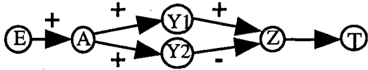
Example 1 In the network shown below, we have (a) s+(Yl, Zlle, Y 2 ) and s-(Y2, Zlle, Y l ) for any e, (b) CI(Z, {E, Yl, Y2}, A), (c) [ E, A, Yl, Y2] is an ancestral ordering, and (d) Yl is not a descendant ofY2 and vice versa. Therefore, we can obtain a lower bound of F(zje) for any E = e by strengthening F(ylja) or weakening F(y2ja) with respect to A.
Theorem I can be applied to cases where we strengthen and weaken multiple such F(yija, px(Yi)), as long as these strengthening and weakening operations are coordi nated consistently so that the effects are to find a lower or an upper bound of F(zje). This extended interpre tation of the theorem can be proved inductively as fol lows. The theorem dictates that we obtain a bound of the exact F(zje) by strengthening or weakening one par ticular F(yija,px(Yi)). In addition, we can obtain a new bound of F(zje) by strengthening or weakening one more such F(yija,px(Yi)) in the ABN where (n -1) F(yija,px(Yi))has been strengthened or weakened. Therefore, by induction, we may coordinate the strength ening and weakening operations to obtain lower (or upper) bounds of F(zje) by strengthening or weakening the con ditional probability distributions of all nodes in Y with re spect to A.
The first condition of Theorem I requires that y i have a non-ambiguous qualitative relationship with Z. This quali tative relationship determines the selection of strengthening and weakening operations for computing desired bounds. The remaining conditions ensure that we can compute desired bounds by locally modifying F(yija,px(Yi)). Specifically, when A has multiple child nodes Y, we can, simultaneously and independently, strengthen or weaken the conditional probability distribution of each node in Y
to obtained bounds of F(zie). Notice that this and the fol lowing theorem do not require a decisive qualitative rela tionship between the evidence nodes E and the node of interest z.
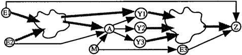
Example 2 Theorem 1 may be applicable to networks that are as complex as the one shown below. In this network, we assume all links point from the left to the right hand side, and we use thick gray links to represent bunches of links that might exist between clouds of nodes and individ ual nodes. WithE = {El, E2, E3}, we can verify that CI(Z, { E, Y}, A) holds in this network. Also, [ E , A, Y] is an ancestral ordering, and yi is not a descendant of SB(Yi) for all yi_ Therefore, Theorem 1 is applicable to any yi that satisfies the first condition in the theorem.
Theorem 1 cannot be applied to cases where A is a parent node of Z because Y and Z represent distinct nodes. The following theorem specifies conditions and methods for ab stracting the parents of Z to compute bounds of F(zie).
Theorem 2 In addition to Conditions 3 and 4 of Theo rem 1, assume that Z E Y. We obtain, respectively, a lower and an upper bound of F(zie) by strengthening and weakening F ( z I a, px ( Z)) with respect to A.
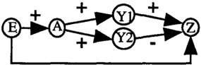
Example 3 In the network shown in Figure 2, we have (a) [E, Yl ,Z] is an ancestral ordering and (b) Z is the only de scendant of Yl. Therefore, Theorem 2 is applicable, and we can obtain a lower bound of F(zie) by strengthening F(ziyl) with respect to Yl. Analogously, we obtain a lower bound of F(zie) by strengthening F(ziy2) with re spect to Y2.
Theorems and 2 also provide guidelines for obtaining tighter bounds. For convenience, if H(x) FSD G(x) FSD F(x), we say that G(x) is less dominating than H(x). Roughly speaking, the following corollary, which follows from Theorem 1, states that we can obtain tighter bounds of F(zie) by setting F(yila,px(Yi)) to a less (or more) dominating alternative.
Corollary 1 Let G(yila , px( Y i)) and H(yila , p x( Y i)) be alternatives for weakening F(yila,px(Yi)) with re spect to A. Assume that H(yila,px(Yi)) is less domi nating than G(yila,px(Yi)) for all a and px(Yi). Then, weakening F(yila , px( Y i)) by G(yii a, px( Y i)) rather than H(yila,px(Yi)) provides a tighter lower bound of F(zie) when <Ti = -,and a tighter upper bound of F(zie) when <Ti = +.
Analogously, strengthening F(yiia, p x( Y i)) by a less dominating CDF provides a tighter upper bound of F(zie) when <Ti = -,and a tighter lower bound of F(zie) when (ji = +.
Similarly, we may derive the following corollary from The orem 2. This corollary provides guidelines for obtaining tighter bounds in applying Theorem 2.
Corollary 2 Applying Theorem 2, we obtain tighter lower (upper) bounds of F(zie) by setting F(zla,px(Z)) to a less (more) dominating alternative.
Notice that neither Theorem 1 nor Theorem 2 requires any particular qualitative relationship between A and nodes in Y. As we mention in Section 4.1, the existence of a par ticular qualitative relationship between A and nodes in Y facilitates, but is not required for, the application of the the orems.
4 State-space abstraction
In previous work, we report an iterative state-space ab straction (ISSA) algorithm for approximate evaluation of Bayesian networks (Wellman & Liu 1994). The ISSA al gorithm aggregates states of variables into superstates to construct abstract versions of the original Bayesian net works (OBNs) that specify exact probability distributions. We use these abstract Bayesian networks (ABNs) to com pute point-valued approximations of the probability distri butions of interest.
To construct ABNs, we select some nodes, called ab stracted nodes, from the OBNs, and aggregate their states. As a result of state aggregation, we need to assign the CPTs of both the abstracted nodes and their child nodes. We call the method used in this assignment task a CPT assignment policy. In this section, we introduce the dominance policy for computing bounds of CDFs.
4.1 Dominance policy
Recall that we need to assign the CPTs of the abstracted node and its child nodes when we abstract a node. The dominance policy modifies the CPT of the abstracted node A as follows:
where P A(A) is the set of parents of A, and [ak,t] is the superstate representing the aggregation of states from ak through at, k � l.
We may choose to strengthen or weaken selected condi tional probability distributions, depending on whether we want to compute lower or upper bounds of the desired CDFs. Let Y be a child node of A, and P X (Y) be the subset of parent nodes of Y excluding A. If we choose to strengthen the conditional probability distributions of Y with respect to A, we assign the CPT of Y as follows.
If we choose to weaken the conditional probability distri butions of Y with respect to A, we assign the CPT of Y as follows.
We need to compare the probability values of the states a;, j = k, l, aggregated in a superstate [ak,d in the OBNs and ABNs in order to apply the aforementioned the orems in analyzing the effects of the dominance policy. In terms of Theorem 1, we want to strengthen or weaken F(yija,px(Yi)) to obtain desired bounds when we ab stract node A. However, A in an ABN has fewer states than A in the OBN, so for a superstate [ak,z]. we do not have cor responding Pr(yila;,px(Yi)) for all j = k, l in the ABN. Fortunately, we may show that the strengthening and weak ening operations in the dominance policy have the effects of strengthening and weakening distributions that we de fined at the beginning of Section 3. We show this by trans forming the ABNs into equivalent networks and comparing these equivalent networks with the OBNs. The procedure for constructing equivalent networks of ABNs and related proofs are available in the full paper.
Application of (2) and (3) becomes easier when the links from the abstracted node to its child nodes can be marked with decisive qualitative signs. For instance, if the sign from A toY is"+", the right hand sides of (2) and (3) are simply F(yja,,px(Y)) and F(yjak,px(Y)), respectively. However, the application of (2) and (3) does not require any particular qualitative relationship between A andY.
4.2 Single node abstraction
In this section, we report the application of the ISSA algo rithm to computing bounds of distributions using qualita tive relationships among nodes. We discuss the application of Theorems 1 and Corollary 1. The application of Theo rem 2 and Corollary 2 is analogous.
We operationalize Theorem 1 using the state-space abstrac tion methods. To compute bounds of the desired CDFs F(zle), we can abstract the state space of any node A that meets the conditions of the theorem. We may apply the in ference algorithms for QPNs (Druzdzel & Henrion 1993) to locate those nodes whose children have unambiguous qualitative relationships with Z as specified in the first con dition of the theorem. We apply (1) to assign the CPT of A, and we apply (2) or (3) to assign the CPTs of the child nodes of A. The selection of (2) or (3) depends on whether we want to compute lower or upper bounds of the desired CDFs, and Theorem 1 provides guidelines for the selection.
The CDF F(zle) specified in the ABNs constructed in this manner is a bound of the CDFs of the F(zle) specified in the OBNs. This is due to Theorem 1 and the fact that we can show that the effects of applying the dominance policy in abstracting nodes are equivalent to strengthening (or weakening) the conditional probability distributions of the children of the abstracted nodes.
We can show that ISSA returns bounds that tighten in each iteration using Corollary 1. The tightening bounds are due to the fact that, as we split superstates, the reassigned CDFs, respectively, become less and more dominating when we strengthen and weaken the orig inal CDFs. Consider the case in which we want to strengthen F(yja,px(Y)) with respective to A. When we split the superstate [ak,d into two superstates [ak,m ] and [am+l,d· m E (k, l), F(yj[ak, t ],px(y)) is replaced with F(yj[ak,m],px(y)) and F(yj[am+1,z ] ,px(y)). We can easily verify that F(yj[ak,!],px(y)) is not larger than F(yi[ak,m],px(y)) and F(yi[am+l,t], px(y)) with (2). As a result, the newly reassigned CDFs are less dominating, and, according to Corollary 1, the bounds of F(zle) tighten in each iteration of ISSA.
4.3 Multiple node abstraction
We may compute bounds of CDFs by abstracting multiple nodes that do not share child nodes. With an analogous method used in the previous section, we can show that the bounds obtained by evaluating network with multiple ab stracted nodes tighten as we split superstates.
Without loss of generality, we may assume that the pur pose of abstracting nodes is to compute an upper bound of F(zle). We analyze the effects of abstracting multiple nodes by assuming that we abstract one node at a time and that we abstract nodes Ai, i = 1, 2, ... , m. Let ABN i de notes the ABN that is constructed by sequentially abstract ing node A1 up to node Ai. Clearly, by applying the result from the previous section, the F(zle) specified in ABN i is an upper bound of the F(zle) specified in ABNi-1 since one more node is abstracted in ABN i than in ABN i - 1 . Therefore, by induction, we can show that the F(zle) spec ified in ABNm is an upper bound of the F(zle) specified in the OBN.
The remaining problem is to show that the ABNm that is constructed by sequentially abstracting node A 1 through A m is the same as the ABN that is constructed by simul taneously abstracting all A i s. Recall that we use maximal
and minimal operations for strengthening and weakening CDFs in (2) and (3). As a result, the order that we abstract the nodes matters only when the abstracted nodes share child nodes. When abstracted nodes share child nodes, ab stracting nodes in different orders may result in different abstract networks due to the fact that maximal and mini mal operations are not commutative. However, when the abstracted nodes do not share child· nodes as in our case, the ordering of these nodes being abstracted will not affect the resulting network, and the ABN m that is constructed by sequentially abstracting node A 1 through Am is the same as the ABN that is constructed by abstracting all A i s in any order. Therefore, we have shown that we can abstract mul tiple nodes that do not share child nodes to obtain bounds of CDFs.
4.4 Generalized qualitative relationship
We can extend the applicability of the theorems by re laxing the required qualitative relationship. Consider the CDF F(ylx, c), where c denotes instantiations of condi tioning variables other than x. Assume that X has m states, x 1 ,x2, . . . , x m . We use S ;t" (X,Y I Ic) to denote the situa tion in which F(ylx, c) has the following property: n is the smallest integer such that, for any y, i E [1, m], j E [n,m),i + j:::; m,
Analogously, we use S;;(X, Yllc) to denote the situation in which F(ylx, c) has the following property: n is the smallest integer such that, for any y, i E [1, m J, j E [n,m),i + j:::; m,
Notice that Si(X, Yllc) and S:l (X, Yllc) correspond to s+(X, Yllc) and s-(x, Yllc), respectively.
With the generalized qualitative relationship, we may extend the applicability of the reported theo rems. Assume that the qualitative relationship be tween yi and Z is s�'(Yi,ZIIe,SB(Yi)) rather than scr' (Yi, Zlle, SB(Yi)). To obtain bounds of F(zle), we need to replace F(zle, y) by F(zle, y) such that F(z!e, y) 2': F(zle, y) for all z and y and that scr'(Yi,ZIIe,SB(Yi)) holds in the abstract network. When the values of F(zle, y) are available, we may be able to replace F(zle, y) in such a manner, and we may apply the theorems to compute bounds of F(zle).
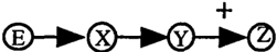
Assume that we have st ( Z, T) in the network shown in following figure, and consider the task of computing bounds of F(tle). In this case, none of the reported theo rems are applicable as they are stated. However, assuming that Z has three possible states, we may replace F(t!z) us ing the following method to create an approximate version of the network in which s+ ( Z, T) holds.
As a result, we have (a) F(tle, yl, y2) 2': F(tle, y1, y2) for all y1 and y2, s+(Y1, Tile, Y2) and s-(Y2, Tile, Y1) in this approximate network, and we may apply the theorems to compute upper bounds of the the actual F(tle) using this approximate network.
In addition, the generalized qualitative relationship sim plifies the strengthening and weakening operations. For instance, if we have S�(A, Yi), the right hand sides of (2) and (3) become minjE[I - n +l,t] F(ylxj,pa(Y)) and maxiE[k,k+n-1] F(ylxi, pa(Y) ) , respectively.
5 Potential Applications
We can apply the ISSA algorithm along with existing in ference algorithms for QPNs (Wellman 1990; Druzdzel & Henrion 1993) for qualitative probabilistic inference. For instance, bounds of probability distributions can be used to resolve ambiguous qualitative relationships between vari ables in QPNs. We report applications of bounds to this task in another paper (Liu & Wellman 1998).
We may also combine the ISSA algorithm with inference algorithms with QPNs to return purely qualitative solu tions and incrementally more precise numerical solutions. Assume a Bayesian network in which links are already marked with qualitative signs. After we infer qualitative re lationship between variables, we may want to know some thing about the numerical relationship between these vari ables. The ISSA algorithm can compute monotonically tightening bounds of conditional CDFs.
The tightening bounds of CDFs allow us to compute tight ening intervals for the expected values of variables. The expected value of a variable Z is Iz z d F(zle). There fore, by Theorem 3, the intervals for the expected value of Z must tighten, if we compute the expected value using the lower and upper bounds of F(zle).
Theorem 3 (cf. (Fishburn & Vickson 1978)) Let g(x) be a monotonically increasing function of a random vari able X, and F(x) and F'(x) denote two cumulative dis tribution functions of X. Then, F(x) FSD F'(x) iff I g(x ) d F(x) 2': I g(x ) d F' (x ).
·
The tightening intervals for expected values can be use ful for applications that use monotone decisions (Wellman 1990). Let the function <5u ( x) choose the value of decision variable D to maximize the utility u for a variable x.
It can be shown that <5u ( x) increases monotonically in x if u is a supermodular function (Ross 1983).
Definition 4 A function u is called supermodular if, for all d1 � d2 andx1 � x2: u(d1,x2)+u(d2,x1) � u(d1,x1)+ u(d2, x2).
A common example of supermodular functions is the util ity function defined as the negative of the squared-error loss function L(d,x) = (d- x) 2 (cf. (Berger 1985)). The tightening intervals for the expected values of X imply that the range of D in which the optimal d exists is decreasing, thereby helping decision makers to focus on fewer alterna tives of D in applications with monotone decisions.
In addition, our theorems can be used to compute the bounds of travel costs on stochastically consistent trans portation networks defined in (Wellman, Ford, & Larson 1995). We can apply our theorems to compute bounds of travel costs, and extend the applicability of our theorems to a broader class of transportation networks, using the gener alized qualitative relationships defined in Section 4.4.
6 Related work
Our approach is similar to many existing algorithms for computing bounds of probability values in that we ig nore some information that specifies the exact distribu tions of Bayesian networks in the computation. For in stance, bounded conditioning ignores some cutset instance to compute probability bounds and consider more instances to improve the bounds (Horvitz, Suermondt, & Cooper 1989). Search-based algorithms search more probable as signments of all variables and use these instances to com pute probability bounds. The bounds can be improved by considering more instances that are less probable (Poole 1993). The incremental term computation method takes advantage of the idea of more probable instances but uses a different strategy to compute the bounds (D'Ambrosio 1993). The localized partial evaluation algorithm removes selected nodes from networks to compute probability in tervals and recovers selected nodes to improve intervals (Draper & Hanks 1994). Our algorithm ignores some dis tinction of states of selected variables to compute approx imations and recovers distinction of states to improve the approximations.
Similar to some other algorithms, ours assumes spe cial numerical properties of the underlying distributions of Bayesian networks. For instance, Poole (1993) and D'Ambrosio (1993) design algorithms that are best for networks with skewed distributions. Jaakkola and Jor dan (1996) develop techniques for computing bounds of likelihood for sigmoid Bayesian networks. Our algorithm requires the existence of qualitative relationships among some variables.
Some algorithms use the maximal and minimal values of a set of numbers in computing the desired bounds. For instance, the mini-buckets algorithm uses maximizing and minimizing functions to bound the values of functions for mini-buckets (Dechter 1997). Our algorithm is more close to Poole's method (1997), but we use bounds of conditional CDFs and Poole uses bounds of conditional probability val ues.
Our algorithm is different from existing algorithms in some aspects. First, we directly compute the bounds of condi tional CDF of interest, i.e., F(zie). In contrast, some algo rithms (Dechter 1997; Poole 1997) compute upper (lower) bounds of Pr(zle) by dividing upper (lower) bounds of Pr(z, e) by lower (upper) bounds of Pr(e) . Another differ ence is that we compute bounds using point-valued infor mation rather than propagating bounds in the computation (Draper & Hanks 1994). Finally, we require the networks be specified with point-valued probabilistic information. We compute bounds of CDFs rather than exact CDFs for saving computational cost. The imprecision is an artifact of the computation algorithm. There is a school of research that works on modeling uncertain situations using proba bility intervals or other alternatives, and they also study al gorithms for computing probability intervals (Walley 1991; Thone, Gtintzer, & KieBling 1992; Chrisman 1996; Luo et al. 1996; Cozman 1997).
7 Summary
We report an application of an extended version of our ISSA algorithm for computing lower and upper bounds of conditional cumulative distribution functions of interest. The algorithm takes advantage of qualitative relationships among variables for bounding the distributions. We show that the bounds tighten monotonically with iterations of computation, thereby providing a guarantee for improving quality of approximations for anytime computation. In par ticular, when used in applications with supermodular utility functions, the monotonically tightening bounds help reduce the set of decision alternatives in each iteration of the ISSA algorithm.
References
Berger, J. 0. 1985. Statistical Decision Theory and Bayesian Analysis. Springer-Verlag.
Boddy, M., and Dean, T. L. 1994. Deliberation scheduling
for problem solving in time-constrained environments. Artificial Intelligence 67:245-285.
Chrisman, L. 1995. Incremental conditioning of lower and upper probabilities. International Journal of Approx imate Reasoning 13:1-25.
Chrisman, L. 1996. Propagation of 2-monotone lower probabilities on an undirected graph. In Proceedings of the Twelfth Conference on Uncertainty in Artificial Intel ligence, 168-184.
Cozman, F. 1997. Robustness analysis of Bayesian net works with local convex sets of distributions. In Proceed ings of the Thirteenth Conference on Uncertainty in Arti ficial Intelligence, 108-115.
Dagum, P., and Luby, M. 1993. Approximating proba bilistic inference in Bayesian belief networks is NP-hard. Artificial Intelligence 60:141-153.
D'Ambrosio, B. 1993. Incremental probabilistic infer ence. In Proceedings of the Ninth Conference on Un certainty in Artificial Intelligence, 301-308. Washington, DC: Morgan Kaufmann Publishers.
Dechter, R. 1997. Mini-buckets: A general scheme for generating approximations in automated reasoning. In Proceedings of the Fifteenth International Joint Confer ence on Artificial Intelligence, 1297-1302.
Draper, D. L., and Hanks, S. 1994. Localized partial evaluation of belief networks. In Proceedings of the Tenth Conference on Uncertainty in Artificial Intelligence, 170177.
Druzdzel, M. J., and Henrion, M. 1993. Efficient reason ing in qualitative probabilistic networks. In Proceedings of the Eleventh National Conference on Artificial Intelli gence, 548-553.
Fishburn, P. C., and Vickson, R. G. 1978. Theoretical foundations of stochastic dominance. In Whitmore, G. A., and Findlay, M. C., eds., Stochastic Dominance: An Ap proach to Decision Making Under Risk, 39-113. Lexing ton, MA: D. C. Heath and Company.
Henrion, M. 1988. Propagating uncertainty in Bayesian networks by probabilistic logic sampling. In Lemmer, J. F., and Kanal, L. N., eds., Uncertainty in Artificial In telligence 2. Elsevier Science Publishers. 149-163.
Horvitz, E. 1990. Computation and Action Under Bounded Resources. Ph.D. Dissertation, Stanford Univer sity.
Horvitz, E.; Suermondt, H. J.; and Cooper, G. F. 1989. Bounded conditioning: Flexible inference for decisions under scarce resources. In Proceedings of the Fifth Work shop on Uncertainty in Artificial Intelligence, 182-193.
Jaakkola, T. S., and Jordan, M. I. 1996. Computing upper and lower bounds on likelihoods in intractable networks.
In Proceedings of the Twelfth Conference on Uncertainty in Artificial Intelligence, 340-348.
Liu, C.-L., and Wellman, M. P. 1998. Incremental tradeoff resolution in qualitative probabilistic networks. In Pro ceedings of the Fourteenth Conference on Uncertainty in Artificial Intelligence.
Luo, C.; Yu, C.; Lobo, J.; Wang, G.; and Pham, T. 1996. Computation of best bounds of probabilities from uncer tain data. Computationallntelligence 12:541-566.
Neal, R. M. 1993. Probabilistic Inference Using Markov Chain Monte Carlo Methods. Ph.D. Dissertation, Univer sity of Toronto, Canada.
Neapolitan, R. E. 1990. Probabilistic Reasoning in Expert Systems: Theory and Algorithms. Wiley.
Pearl, J. 1987. Evidential reasoning using stochastic sim ulation of causal models. Artificial Intelligence 32:245257.
Poole, D. 1993. Average-case analysis of a search al gorithm for estimating prior and posterior probabilities in Bayesian networks with extreme probabilities. In Pro ceedings of the Thirteenth International Joint Conference on Artificial Intelligence, 606-612.
Poole, D. 1997. Probabilistic partial evaluation: Exploit ing rule structure in probabilistic inference. In Proceed ings of the Fifteenth International Joint Conference onAr tificiallntelligence, 1284-1291.
Ross, S. M. 1983. Introduction to Stochastic Dynamic Programming. Academic Press.
Thone, H.; Giintzer, U.; and KieBling, W. 1992. To wards precision of probabilistic bounds propagation. In Proceedings of the Eighth Conference on Uncertainty in Artificial Intelligence, 315-322.
van Engelen, R. A. 1997. Approximating Bayesian belief networks by arc removal. IEEE Transactions on Pattern Analysis and Machine Intelligence 19(8):916-920.
Walley, P. 1991. Statistical Reasoning with Imprecise Probabilities. Chapman and Hall.
Wellman, M. P. 1990. Fundamental concepts of qualita tive probabilistic networks. Artificial Intelligence 44:257303.
Wellman, M. P., and Liu, C.-L. 1994. State-space abstrac tion for anytime evaluation of probabilistic networks. In Proceedings of the Tenth Conference on Uncertainty in Artificial Intelligence, 567-574.
Wellman, M. P.; Ford, M.; and Larson, K. 1995. Path planning under time-dependent uncertainty. In Proceed ings of the Eleventh Conference on Uncertainty in Artifi cial Intelligence, 532-539.