Using the structure of d-connecting paths as a qualitative measure of the strength of dependence.

Sanjay Chaudhuri

Department of Statistics University of Washington Seattle, WA 98195

Abstract

Pearl's concept of a d-connecting path is one of the foundations of the modern the­ ory of graphical models: the absence of a d-connecting path in a DAG indicates that conditional independence will hold in any distribution factorizing according to that graph. In this paper we show that in singly­ connected Gaussian DAGs it is possible to use the form of a d-connecting path to obtain qualitative information about the strength of conditional dependence. More precisely, the squared partial correlations between two given variables, conditioned on different sub­ sets may be partially ordered by examin­ ing the relationship between the d-connecting path and the set of variables conditioned upon.

1 Introduction

Central to the modern theory of graphical models is the concept of d-separation which provides a simple algorithm for determining which conditional indepen­ dence relations will hold in a distribution factorizing according to a DAG. Completeness results [4] , [7] show further that whenever a d-connecting path exists be­ tween x and y given Z in a DAG G then in 'almost all' distributions that factor according to G, x and y will be dependent given Z.

However, recent work has shown that not all d­ connecting paths are created equal : Greenland [ 5 ] shows that in certain specific contexts relevant to causal analysis in Epidemiology, shorter d-connecting paths lead to qualitatively stronger dependence than longer paths.

In this paper we analyse the relationship between the strength of dependence resulting from a single

Thomas Richardson

Department of Statistics University of Washington Seattle, WA 98195

d-connecting path and the set of variables which have been conditioned on in the situation where the joint distribution is Gaussian and the DAG is singly­ connected.

Since colliders are made 'active' by conditioning on their descendants it seems as if the strength of depen­ dence ought to be inversely related to the length of the path from a collider to a vertex in the conditioning set. Likewise one would expect dependence to decrease if we condition on vertices 'near' to a non-collider on a path. Such intuitions are given additional impetus by the intuitive description of d-separation in terms of 'causal pipes' ([9], p. 72). However, our analysis shows that though there are situations in which these intu­ itions are correct (Lemmas 3.1 and 3.2) there are also contexts where these intuitions are either incorrect or provide no guidance (Lemmas 3.3 and 3.4).

An understanding of the relationship between the graphical structure and strength of dependence will facilitate sensitivity analysis in causal inference and may suggest new strategies for constraint based search [3],[2].

The paper is organised as follows: Section 2 con­ tains the basic definitions; in Section 3 we consider four canonical examples; in Section 4 we define a par­ tial ordering on conditioning sets associated with a d-connecting path; Section 5 describes properties of singly connected DAGs; Section 6 contains the main result and Section 8 a brief discussion. Proofs of the results in Section 3 are in the Appendix.

2 Some Initial Definitions

Let G = (V, E) be a DAG. A non-endpoint vertex (on a path is a collider on the path if the edges preceding and succeeding (on the path have an arrowhead at( , i.e. -t ( t-. A non-endpoint vertex ( on a path which is not a collider is a non-collider on the path. A path between vertices a and f3 in a DAG G is said to be

d-connecting given a set Z (possibly empty) if

(i) every non-collider on the path is not in Z, and

(ii) every collider on the path is in an(Z).

where an(Z) = {x I x -+ · · · -+ z or x =zinG}. If there is no path d-connecting a and f3 given Z, then a and f3 are said to be d-separated given Z. For disjoint sets X, Y, Z, where Z may be empty, X andY are d­ separated given Z, if for every pair a, f3, with a E X and f3 E Y , a and f3 are d-separated given Z.

Let V = { v1, . . . , Vn}. When the joint distribution is normal the model may be expressed by the following equations

where pav; is the vector of parents of v; and hv; is the vector of coefficients bv, v ; , Vj E pa( v;). tv, follows a N(o , r ; J distribution. The joint variance-covariance matrix for V is given by :

where

We assume that l bv, v ; I > 0 if Vj E pa(v; ) and r ; , > 0 so Ev is positive definite .

We use p� CIB as our measure of association of A and C conditional on B. Note that it is a monotonic trans­ formation of the information proper of the conditional independence of A and C given B. The information proper for normal models takes the form

we cite [10] for details.

For vertices X, Y and a collection of vertices Z by axYIZ and axx1z we denote respectively the condi­ tional covariance between X and Y given Z and the conditional variance of X given Z. Note that Z may be 0. If X and Y are each a collection of vertices, then Exy will denote the X x Y sub-matrix of Ev in ( 2). Throughout this article we shall repeatedly use the expression for conditional covariance in the Gaussian case:

This easily gives the expression for the conditional cor­ relation and regression coefficients (see [6]). More gen­ erally if X1, X2, . . . , X p jointly follows a N(J.t, E ) dis­ tribution then the iterative expression

holds. Similar iterative expressions exist for the con­ ditional correlation and regression coefficients. (see [6](page 346) or [1]).

3 Canonical examples

We start by looking at some specific key cases. The motivation for this being the fact that later it will be shown that a more general case can be reduced to these. Proofs are in the appendix.

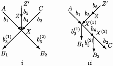
Lemma 3.1. In the graph in figure l.i

holds, or in other words the squared correlation de­ creases with proximity to the path.

Note that this fits with the intuition that the closer we are to X, the more nearly we block the A -C path. The result directly generalises to a graph in which . . . . Z.

Lemma 3.2. In the graph in figure l.ii

holds, where B is a set of descendants of X or in other words the squared correlation increases with proximity to X. (In Fig l.ii, B = {Bt,B2}.)

Again this fits the intuition that the further we move from the path the weaker is our information about X and hence the closer we are to d-separating.

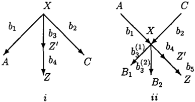
Lemma 3.3. In the graph in figure 2.i

holds, where B = {B1,B2} or in other words the squared correlation increases with proximity to vertex X.

Lemma 3.4. In the graph in figure 2.ii

holds, where B is a set of descendants of X(l), or in other words the squared correlation increases with proximity to vertex X(!), though conditioning on X(I) d-separates A and C.

The following is an extension of the graph in figure 2.ii.

c

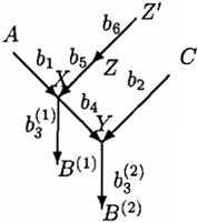
Lemma 3.5. In the graph in figure 3

holds, where B is a set of descendants of XU Y, or in other words the squared correlation increases with proximity to vertex X, though conditioning on X d­ separates A and C.

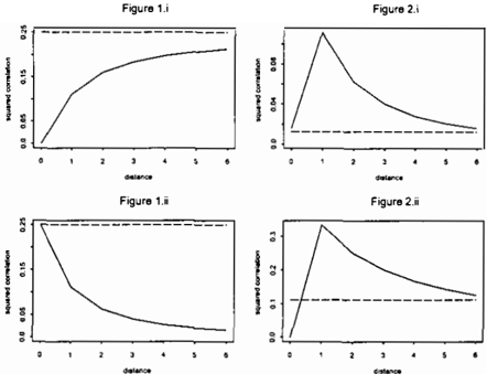
In figure 4 we plot the squared correlation for the above cases as we increase the length of the path between X and Z. Figure l.i is for the graph in figure l.i. Figure l.ii is for that in figure l.ii, with B = 0. Figure 2.i is for figure 2.i with IBI = 1 and the last figure in the plot is for figure 2.ii with B = 0. All the parameter values are fixed at 1. In the plot the curved lines show the values of the squared correlations. The broken lines denote P�c in case of figure l. i , P�crx in figure l. ii , P�c[B in figure 2.i and P�c in figure 2.ii. In the Figure 2.i we also note that the value of P�c[x is larger than the p�CIB as expected from Lemma 3.2, also it seems that that the solid curve in this plot converges to P�crx·

diglance distance

Figure 4 : Squared correlation as a function of distance from the path to the vertex conditioned on (see text for explanation)

4 A partial ordering on conditioning sets associated with a path

Building on the previous examples we now construct a partial ordering on conditioning sets associated with a specific path. Let G = (V, E) be a singly connected DAG i.e. the adjacencies in G form a tree. Let A and C be two nodes A ¥ C. By a path A 7r c we mean a sequence of non repeating adjacent nodes {X I , x2, . . . , Xn} <;; V s.t. X! = A and Xn = C. Since G is singly connected for any two vertices A, C, A ,PC there is a unique A 7r c connecting A and C.

Define 2z = the power set of Z. Below we shall use graphical structure to define a partial order on 2z. Let Z denote an element in 2z.

Since G is tree structured then for any z E Z there is a unique x� E A'Trc so that A'Trz n c'Trz n A'Trc = x�. For each Z E 2z define

We further subdivide Zc in two parts :

• Zc-c ={ z E Z : at least one of c7r z ,A 7r z has a collider at x�}, (11)

Note that in definitions (11) and (12) if for some z E Zc, z = x�, then since A 7r z and c7r z do not have colliders at z, (endpoints are neither colliders nor non­ colliders) there is a collider at z in A1r c . So z E Zc-nc·

Let z E Znc, then define z to be a nearest vertex to A 7r c in Znc if there is no z' # z E Znc s.t. z' E A1rz n c7rz. Let

Similarly we define :

N (Zc-c) = set of all nearest nodes to A 7r c in Zc-c, N (Zc-nc) =set of all nearest nodes to A 7r c in Zc-nc·

Let S 1 ,S 2 E 2z. Then (5 2 ,5 1 ) is a total further­ nearer pair w.r.t. A1r c if

1. For each Z 2 E 5 2 , 3 Z l E 5 1 s.t. z1 E A 7r z 2 n c7r z 2 ·
2. For each z 1 E 5 1 , 3 Z 2 E 5 2 s.t. z1 E A 7r z 2 n c7r z 2 ·

Let ;z(ll,Z( 2 ) E 2 z . We define ;z(l)-< Z( 2) E 2z if all the following are satisfied :

• (i) ( N ( zl?J) , N ( Z � 1 J)) is a total further - nearer pair w.r.t. A1r c .
• (ii) ( N ( Z��c) , N ( Z��c)) is a total further - nearer pair w.r.t. A1r c .
• (ii) (N(z��nc),N(z��nc)) is a total further nearer pair w.r.t. A1rc .

-

5 Some facts about singly connected DAGs

As before let G = (V, E) be a singly connected DAG and A 7r c be a path between two nodes A =I C.

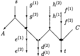
Figure 5: Example of two ordered conditioning sets: ;z(ll = {s, g(ll, e( 1 l, d(ll, h( 1 l, f(ll, t}-< ;z( 2 ) = {s, g( 2 ), e( 2 ), d( 2 ), h( 2 ), f( 2 ), t}. Here Z� 1 J = { e(l), h( 1 ), s} ;z ( 2 ) = {e( 2 ) h( 2 ) s} ;z (l) = {g(l) f(l)} ., ( 2 ) = l nc ' ' c-c l ' ILl c-c {g( 2 ), f( 2 )}, Z��nc = {d(l), t}, Z��nc = {d( 2 ), t}, .

Lemma 5.1. For any y,z E V, y # z, [pa(y) n pa(z)[ :::; 1 and [ch(y) n ch(z)[ :::; 1. Moreover at most one of pa(y) n pa(z) and ch(y) n ch(z) is nonempty. Also Vx E V, x � y 7r z , then there exists at most one wE y 1rz so that x E pa(w) or x E ch(w).

Proof. If there are two common parents say x, x* then the skeleton of the subgraph G{x,x·,y,z} has a 4 cycle, which violates the assumption. Similar proof follows for common children.

The second part follows from the fact that if both of pa(y)npa(z) and ch (y) n ch ( z ) are non empty then the skeleton of G has a 4 cycle.

Similar arguments prove the other statements. D

Lemma 5.2. Let G = (V, E) be a singly connected DAG. Let G* be the induced subgraph consisting of y 7r z , (y =I z) . Then for disjoint subsets 5t, 5 2 , 53 occurring on y 7r z , 5t is d-separated from 5 2 given 53 in G* iff 5t is d-separated from 5 2 given 53 in G.

Proof. The proof is intuitively clear. For a detailed proof see Theorem 4.18 in [8] . D

Lemma 5.3. Let G = (V, E) be a singly connected DAG. Then if Z <; V, there exists a DAG G* = (V \ Z, E*) such that for disjoint 5t, 5 2 , 53 <; V \ Z (53 may be empty) 5t and 5 2 are d-separated given 53 u Z in G iff 5t and 5 2 are d-separated given S3 in G*

Proof. The proof follows from Theorem 4.18 and The­ orem 4.2 in [ 8]. D

In other words given a singly connected DAG G and a set Z we may always find a new DAG G* whicil represents the d-separation relations holding in G after conditioning on Z.

6 The main theorems

Let G = (V, E) be a singly connected DAG, A, C E V, A iC. Let z ( l l , z< 2 l E 2z, so that z<t)-< z< 2 l. The main result of this section is that p � CIZ<I> � P � ci z <2 >·

Proof. Let P � cl z < 2> = 0. Since by assumption lbv,p a (v , )i > 0 and TJ, > 0, Vv; E V it follows that A and C are d-separated given Z ( 2 ). Then either there is a non-collider x on the path which is in Z ( 2 ) or there is a collider x which has no descendants in Z ( 2 ).

Case 1. If x is a non-collider on A 7T" c then since X is an endpoint of A 7T" x and c7T" x , X \t /l� 2 ) , hence X E Z� 2 J. Since x* = X, X E N ( Z� 2 J) and since ( N ( z\?J) , N ( z�J)) is a total further­ nearer pair, so by ( a ) of the definition there is ( (1) ) some yEN Znc s.t. y E A1T"x n c1T"x . Hence x E N ( Z� 1 d) <:::; Z� 1 d, since the paths only inter­ sect at x. Thus A and C are d-separated given z< t J.

Case ( 2 ) : If there is a collider X s.t. de ( x ) n.Z( 2 ) = 0, then since the collider is in A1T" c then de ( x ) n z�::! c = 0 by construction and de ( x ) n z�::!nc = 0 by assumption. Thus de ( x ) n N (Zc-nc) = 0.

Now as (N(z��nc),N(z�::!nc)) form a total further-nearer pair so by ( b ) of the definition there is no de ( x ) in Z��nc· Thus by single connected­ ness de ( x ) nz<t) = 0. Note that de ( x ) nz��c = 0. So A and C are d-separated given z<1l.

We have shown that in this case p � Ci z < 1 > = 0. D

Assume P � ci z < 2> > 0. If z { i ) contains a non-collider in A 1T" c trivially P � cl z < · > = 0, i = 1, 2. Thus we can assume that none of z(t) and z< 2 l contain any non­ collider in A 7T" c .

Let N (Z) = N (Znc) UN (Zc-c) UN (Zc-nc)· Since the graph is singly connected,

So it suffices to show that

First consider the case where k t = k2 = k, I t = l 2 = l and m1 = m 2 = m.

The following theorems are proved by showing that each term in the above product is bounded by 1.

Theorem 2. Let G = (V, E) be a singly connected DAG. A, C E V and A iC. Suppose A1T" c does not have a collider. Let _z( t ) -< z< 2 l and k1 = k2, I t = 12· Then

Proof. ( Sketch ) Note that since A 7T" c does not have a collider then both Z��nc and z�::!nc are empty. So the product ( 16 ) will only have the first two products, more over it will only involve the a and b nodes.

By choosing the nodes to be conditioned on and marginalised out in an appropriate order one can show that it is possible to reduce the graph corresponding to each term in the first product in (16) to a graph Markov equivalent to figure l.i and that in the second product to that in figure 2.ii.

So by Lemma 3.1 and 3.4 the proof follows. D

Theorem 3. Let G = (V, E) be a singly connected DAG. A, C E V and A iC. Suppose A1T" c has exactly one collider. Let z ( l ) -< z< 2 l and k 1 = k2, I t = l 2 , m1 = m 2 . Then

Proof. The proof is similar to the proof of Theorem 2 only in this case we can reduce the graphs in each term of the first product to a graph which is Markov equivalent to the graph in l.i. The terms in the third

product reduce to the DAG in figure l.ii and those of the second one reduce to figure 3 or figure 2.i, depend­ ing on whether one or both of A 1T"bC1l and c1T"bC1l has a collider in x * < , l = x * < ' l . So by th e lemmas in s ection bi bi 3 the theorem follows. D

Theorem 4. Let G = (V, E) be a singly connected DA G. A, C E V and A # C. Suppose A 1T" c has more than one collider. Let z(l ) -< Z( 2 l and k1 = k2, h = 1 2, m1 = m2. Then

Proof. Note that between any two colliders there is exactly one source and conditioning on the nodes on one side of the collider does not change the graph on the other side. Thus one can show that each term in (16) may be reduced to a turn case in which A 1T" c has exactly 1 collider. The proof follows from theorem 3. D

However if k1 # k2, h # l2, m1 # m2. Then by the definition of the ordering and the struc­ ture of G we note that k 1 > k2, h < l2 , m1 < m2. Suppose for instance b(l) E N (Z( 1 l) is such that 3 b\ 2 ) , b� 2 ) E N (Z( 2 l) s.t. b( 1 ) E A 1T" b \ 'l n c?r b \ 'l n A 1T" b \ 'l n c?r b \ 'l . Then we note that as {A, C} Jl b� 2 ) l b( l ) , P�CI{Wl , b� 'l} = P � c!Wl · Thus we redefine N (Z( 1 l) to be N (Z(1 l) U b�2) and reduce this case to the case where k 1 = k2. A similar proof follows when k2 - k1 > 1, h < l2 and m1 < m2.

7 Multiply connected DAG

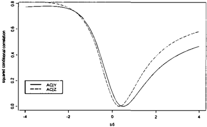
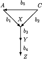
If the graph is not singly connected the ordering of the dependence as described in section 6 may fail. For example consider the graph in figure 6. In figure 7 we plot the squared conditional correlations p � CIY and P � CIZ with bs. Other parameter values are fixed at 1. We note that for b5 = 0 p � CIZ < p � CIY which is a special case for Lemma 3.2. However for smaller and larger values of b5 the opposite inequality is valid. The range of b5 in the plot is [ -4, 4].

8 Discussion

In this paper we have wrung qualitative information about the strength of dependence from the structure of the graph. We believe that it may be possible to strengthen this result by constructing a richer ordering under which more sets would be comparable.

It is also natural to ask whether the result may be ex­ tended to other distributions or classes of graphs. [3]

c

-=��

--,

Figure 7: Squared conditional correlation coefficient with b5 for the DAG in figure 6.

show that discrete distributions exist corresponding to Fig.l.ii in which I(A; C I Z) > I(A; C I Z'), hence Lemma 3.2 will not hold without without additional assumptions. Section 7 shows that non-monotonic de­ pendence orderings may exist in simple multiply con­ nected Gaussian DAGs. However, in spite of this we believe that the relationships shown in Figure 4 sug­ gest the possibility of developing a theory which pro­ vides upper bounds on the strength of conditional de­ pendence which may be present in a given graph.

9 Appendix

By L:"Bk we denote (L:BB) - l and write x ex:+ y if 3 constant K > 0 s.t. x = K y .

Proof of lemma 3.1: Note that

We shall consider in turn the two terms in this prod­ uct and compare them to the corresponding terms in p�CIZ' . Consider first

After combining, the denominator is always positive so the sign of the expression is determined by the nu­ merator which after some simplification is

Since a 2: 1, the above is negative iff b1b2 < 0. Simi­ larly one can show that.

If b1b2 2: 0 then

However

So again

Let K and K1 be constants and for some A, C, D E V and B C V, where B may be empty, define:

Then the sign of d��·) is the sign of the numerator of d�L·). By the quotient rule

Some algebraic simplification yields

Also note that

In the proofs of Lemmas 3.2, 3.3, 3.4, 3.5 we will find constants K and K' such that

In the proof below we shall consider

We shall then re-express (43) in the form of L(a) and note that L(l) = p�CIBZ'" By using the equation (39) we shall determine the sign of �� , thereby drawing conclusions on the values of the squared conditional correlations. For lack of space however we present the proof of lemma 3.4 only. The proofs of lemma 3.2 and lemma 3.3 and Lemma 3.5 follow mutatis mutandis.

proof of Lemma 3.4: Let B = { B 1 , B 2 } . Then for B; E B

aAz = aAz· = 0. Also for Y = {A , C}

2 Then with a = 1/(1 + bi,Z;,) < 1, K' = :Bz'B:Bfik:!:Bz·/r�, and K = 1:Bz·B:Bfik:BBz·/r�, we get

Using (7) and (43) we can show that �ClBZ has the same form as L(a) as in (33). As before L(l) = p�ClBZ'. Then by defining

we get

where ai<·> = ax<·>x<·> and similarly for ai<·>. Simi­ larly we can show

Thus

As Q2, K and (a -K') are positive the sign of �� depends on the sign of -b�b�Q�, which is negative. So L(l) :S: L(a). Thus it follows that :

References

1. C. Brito and J. Pearl. Generalised instrumental vari­ ables. UAI 2002, pages 85-93, 2002.
2. J. Cheng, R. Greiner, J. Kelly, D. Bell, and W. Lin. Learning Bayesian networks from data: an information-theory based approach. Artificial Intelli­ gence, 197:43-90, 2002.
3. D.M. Chickering and C. Meek. Monotone DAG faith­ fulness: a bad assumption. Technical Report MSR­ TR-2003-16, Microsoft Research, 2003.
4. D. Geiger and J. Pearl. On the logic of causal mod­ els. In L. N. Kana! R.D. Schachter, T. S. Levitt and J. F. Lemmer, editors, Uncertainty in the Artificial inteligence IV, pages 136-147. North-Holland, Ams­ terdam, 1990.
5. S. Greenland. Quantifying biases in causal mod­ els: classical confounding versus collider-stratification bias. Epidemiology, 2003. to appear.
6. M. Kendall and A. Stuart. The Advanced Theory of Statistics, vol. 2, Inference and Relationship. Macmil­ lan Publishing Co., Inc., 1979.
7. C. Meek. Strong completeness and faithfulness in Bayesian networks. UAI 1995, pages 403-410.
8. T. Richardson and P. Spirtes. Ancestral graph Markov models. The Annals of Statistics, 30(4):962-1030, 2002.
9. P. Spirtes, C. Glymour, and R. Scheines. Causation, Prediction and Search. Number 81 in Lecture Notes in Statistics. 1993.
10. J. Whittaker. Graphical Models in Applied Mathemat­ ical Multivariate Statistics. John Wiley & Sons, 1989.