--;

Value Function Approximation in Zero-Sum Markov Games

Michail G. Lagoudakis and Ronald Parr

Department of Computer Science Duke University Durham, NC 27708 {mgl,parr}©cs.duke.edu

Abstract

This paper investigates value function approx­ imation in the context of zero-sum Markov games, which can be viewed as a generalization of the Markov decision process (MDP) frame­ work to the two-agent case. We generalize er­ ror bounds from MDPs to Markov games and describe generalizations of reinforcement learn­ ing algorithms to Markov games. We present a generalization of the optimal stopping prob­ lem to a two-player simultaneous move Markov game. For this special problem, we provide stronger bounds and can guarantee convergence for LSTD and temporal difference learning with linear value function approximation. We demon­ strate the viability of value function approxima­ tion for Markov games by using the Least squares policy iteration (LSPI) algorithm to learn good policies for a soccer domain and a flow control problem.

1 Introduction

Markov games can be viewed as generalizations of both classical game theory and the Markov decision process (MDP) framework1. In this paper, we consider the two­ player zero-sum case, in which two players make simulta­ neous decisions in the same environment with shared state information. The reward function and the state transition probabilities depend on the current state and the current agents' joint actions. The reward function in each state is the payoff matrix of a zero-sum game.

Many practical problem can be viewed as Markov games, including military-style pursuit-evasion problems. More­ over, many problems that are solved as classical games

1 Littman (1994) notes that the Markov game framework actu­ ally preceded the MOP framework.

by working in strategy space may be represented more ef­ fectively as Markov games. A well-known example of a Markov game is Littman's soccer domain (Littman, 1994).

Recent work on learning in games has emphasized accel­ erating learning and exploiting opponent suboptimalities (Bowling & Veloso, 2001). The problem of learning in games with very large state spaces using function approx­ imation has not been a major focus, possibly due to the perception that a prohibitively large number of linear pro­ grams would need to be solved during learning.

This paper contributes to the theory and practice of learning in Markov games. On the theoretical side, we generalize some standard bounds on MDP performance with approxi­ mate value functions to Markov games. When presented in their fully general form, these tum out to be straightforward applications of known properties of contraction mappings to Markov games.

We also generalize the optimal stopping problem to the Markov game case. Optimal stopping is a special case of an MDP in which states have only two actions: continue on the current Markov chain, or exit and receive a (possi­ bly state dependent) reward. Optimal stopping is of inter­ est because it can be used to model the decision problem faced by the holder of stock options (and is purportedly modeled as such by financial institutions). Moreover, lin­ ear value function approximation algorithms can be used for these problems with guaranteed convergence and more compelling error bounds than those obtainable for generic MDPs. We extend these results to a Markov game we call the "opt-out", in which two players must decide whether to remain in the game or opt out, with a payoff that is de­ pendent upon the actions of both players. For example, this can be used to model the decision problem faced by two "partners" who can choose to continue participating in a business venture, or force a sale and redistribution of the business assets.

As in the case of MDPs, these theoretical results are some­ what more motivational than practical. They provide re­ assurance that value function approximation architectures

which can represent value functions with reasonable er­ rors will lead to good policies. However, as in the MDP case, they do not provide a priori guarantees of good per­ formance. Therefore we demonstrate, on the practical side of this paper, that with a good value function approximation architecture, we can achieve good performance on large Markov games. We achieve this by extending the least squares policy iteration (LSPI) algorithm (Lagoudakis & Parr, 2001), originally designed for MDPs, to general two­ player zero-sum Markov games. LSPI is an approximate policy iteration algorithm that uses linear approximation architectures, makes efficient use of training samples, and learns faster than conventional learning methods. The ad­ vantage of using LSPI for Markov games stems from its generalization ability and its data efficiency. The latter is of even greater importance for large Markov Games than for MDPs since each learning step is not light weight; it requires solving a linear program.

We demonstrate LSPI with value function approximation in two domains: Littman's soccer domain in which LSPI learns very good policies using a relatively small num­ ber of sample "random games" for training; and, a simple server/router flow control problem where the optimal pol­ icy is found easily with a small number of training samples.

2 Markov Games

A two-player zero-sum Markov game is defined as a 6tuple (S, A, 0, P, n, 'f' ) , where: s = { S), 82, ... , Sn } is a finite set of game states; A = {a 1, a2, ... , am} and 0 = { o1, o2, ... , o! } are finite sets of actions, one for each player; Pis a Markovian state transition modelP(s, a, o, s ') is the probability that s' will be the next state of the game when the players take actions a and o respectively in state s; n is a reward (or cost) functionR(s, a, o) is the ex­ pected one-step reward for taking actions a and o in state s; and, 'Y E (0, 1] is the discount factor for future rewards. We will refer to the first player as the "agent," and the sec­ ond player as the "opponent." Note that if the opponent is permitted only a single action, the Markov game becomes an MDP.

A policy 1r for a player in a Markov game is a mapping, 1r : S --+ O(A), which yields probability distributions over the agent's actions for each state in S. Unlike MDPs, the optimal policy for a Markov game may be stochastic, i.e., it may define a mixed strategy for every state. By conven­ tion, 1r( s) denotes the probability distribution over actions in states and 1r(s, a) denotes the probability of action a in states.

The agent is interested in maximizing its expected, dis­ counted return in the minimax sense, that is, assuming the worst case of an optimal opponent. Since the underlying rewards are zero-sum, it is sufficient to view the opponent as acting to minimize the agent's return. Thus, the state value function for a zero-sum Markov game can be defined in a manner analogous to the Bellman equation for MDPs:

where the Q-values familiar to MDPs are now defined over states and pairs of agent and opponent actions:

We will refer to the policy chosen by Eq. (I) as the minimax policy with respect to Q. This policy can be determined in any state s by solving the following linear program:

In many ways, it is useful to think of the above linear pro­ gram as a generalization of the max operator for MDPs (this is also the view taken by Szepesvari and Littman (1999)). We briefly summarize some of the properties of operators for Markov games which are analogous to oper­ ators for MDPs. (See Bertsekas and Tsitsiklis (1996) for an overview.) Eq. (I) and Eq. (2) have fixed points V* and Q*, respectively, for which the minimax policy is optimal in the minimax sense. The following iteration, which we name with operator T*, converges to Q*:

This is analogous to value iteration in the MDP case.

For any policy 1r, we can define Q rr ( s, a, o) as the expected, discounted reward when following policy 1r after taking ac­ tions a and o for the first step. The corresponding fixed point equation for Qrr and operator Trr are:

A policy iteration algorithm can be implemented for Markov games in a manner analogous to policy iteration for MDPs by fixing a policy 7r;, solving for Qrr,, choosing 1r i + 1 as the minimax policy with respect to Q rr , and iterat­ ing. This algorithm will also converge to Q*.

3 Value Function Approximation

Value function approximation has played an important role in extending the classical MDP framework to solve practi­ cal problems. While we are not yet able to provide strong

a priori guarantees in most cases for the performance of specific value function architectures on specific problems, careful analyses such as (Bertsekas & Tsitsiklis, 1996) have legitimized the use of value function approximation for MDPs by providing loose guarantees that good value func­ tions approximations will result in good policies.

Bertsekas and Tsitsiklis (1996) note that "the Neuro­ Dynamic Programming (NDP) methodology with cost-to­ go function approximation is not very well developed at present for dynamic games"2 (page 416). To our knowl­ edge, this section of the paper provides the first error bounds on the use of approximate value functions for Markov games. We achieve these results by first stating extremely general results about contraction mappings and then showing that known error bound results for MDPs generalize to Markov games as a result. 3.

An operator T is a contraction with rate a with respect to some norm 11·11 if there exists a real number a E [0, 1) such that for all vl and v 2 :

An operator T is a non-expansion if

The residual of a vector V with respect to some operator T and norm II · II is defined as

Lemma 3.1 Let T be a contraction mapping in I I · II with rate a and fixed point V*. Then,

This lemma is verified easily using the triangle inequality and contraction property ofT.

Lemma 3.2 Let 7j and 72 be contraction mappings in 11·11 with rates a1. a2 (respectively) and fixed points Vt and V2* (respectively). Then,

where @3 = max(α1,α2).

This result follows immediately from the triangle inequal­ ity and the previous lemma. A convenient and relatively well-known property of Markov games is that operators T* and T" are contractions in II · l l oo with rate/. where

2 NDP is their term for value function approximation.

3 We thank Michael Littman for pointing out that these results should also apply to all generalized MOPs (Szepesvari & Littman, 1999)

II V IIoo = maxsES IV(s)l (Bertsekas & Tsitsiklis, 1996). The convergence of value iteration for both Markov games and MDPs follows immediately from this result.

Theorem 3.3 Let Q* be the optimal Q function for a Markov game with value iteration operator T*.

This result follows directly from Lemma 3.1 and the con­ traction property of T*. While it gives us a loose bound on how far we are from the true value function, it doesn't answer the more practical question of how the policy corre­ sponding to a suboptimal value function performs in com­ parison to the optimal policy. We now generalize results from Williams and Baird (1993) to achieve the following bound:

Theorem 3.4 Let Q* be the optimal Q function for a Markov game and T* be the value iteration operator for this game. If 1r is the minimax policy with respect to Q, then

This result follows directly from Lemma 3.2 by noting that £p is identical to £y. at this point. As noted by Baird and Williams the result can be tightened by a factor of 1 by ob­ serving that for the next iteration, T* and T" are identical. Since this bound is tight for MDPs, it is necessarily tight for Markov games.

The significance of these results is more motivational than practical. As in the MDP case, the impact of small approx­ imation errors can, in the worst case, be quite large. More­ over, it is essentially impossible in practice to compute the residual for large state spaces and, therefore, impossible to compute a bound for an actual Q function. As with MDPs, however, these results can motivate the use of value func­ tion approximation techniques.

4 Approximation in Markov Game Algorithms

Littman (1994) studied Markov games as a framework for multiagent reinforcement learning (RL) by extending tab­ ular Q-learning to a variant called minimax-Q. By view­ ing the maximization in Eq. (1) as a generalized max op­ eration (Szepesvari & Littman, 1999) minimax-Q simply uses Eq. (1) in place of the traditional max operator in Q­ learning. The rub is that minimax-Q must therefore solve one linear program for every experience sampled from the environment. We note that in the case of Littman's 4 x 5 soccer domain, 10 6 learning steps were used4, which im-

4 It's not clear that this many were needed; but this was the duration the training period.

plies that 106 linear programs were solved. Even though the linear programs were small, this adds further motiva­ tion to the desire to increase learning efficiency through the use of value function approximation.

In the natural formulation of Q-learning with value func­ tion approximation for MDPs, a tabular Q-function is replaced by a parameterized Q-function, Q(s, a, w ), where w is some set of parameters describing our approximation architecture, e.g., a neural network or a polynomial. The update equation for a transition from state s to state s' with action a and reward r then becomes:

where Q is the learning rate.

One could easily extend this approximate Q-learning al­ gorithm to Markov games by defining the Q-functions over states and agent-opponent action pairs, and replac­ ing the max operator in the update equation with the min­ imax operator of Eq. (1 ). This approach would yield the same stability and performance guarantees of ordinary Q­ learning with function approximation, that is, essentially none. Also, it would require solving a very large number of linear programs to learn a good policy. In the following two sections, we separately address both of these concerns: stable approximation and efficient learning.

5 Stable Approximation

A standard approach to proving the stability of a function approximation scheme is to exploit the contraction prop­ erties of the update operator T. If a function approxima­ tion step can be shown to be non-expansive in the same norm in which T is a contraction, then the combined up­ date/approximation step remains a contraction. This ap­ proach is used by Gordon (1995), who shows that a general approximation architecture called an averager can be used for stable value function approximation in MDPs. This and similar results generalize immediately to the Markov game case and may prove useful for continuous space Markov games, such as pursuit-evasion problems.

In our limited space, we choose to focus on an architecture for which the analysis is somewhat trickier: linear approx­ imation architectures. Evaluation of a fixed policy for an MDP is known to converge when the value function is ap­ proximated by a linear architecture (Van Roy, 1998). Two such stable approaches are least-squares temporal differ­ ence (LSTD) learning (Bradtke & Barto, 1996) and linear temporal difference (TD) learning (Sutton, 1988). In these methods the value function V is approximated by a linear combination of basis functions </>i:

We briefly review the core of the convergence results and error bounds for linear value function approximation and the optimal stopping problem. We can view the approxi­ mation as alternating between dynamic programming steps with operator T and projection S _! eps with operator II, in an attempt to find the fixed point V (and the corresponding w):

If the operator T is a contraction and II is a non-expansion in the same norm in which T is a contraction, then w is well-defined and iterative methods such as value iteration or temporal difference learning will converge to w. For linear value function approximation, if the transition model P yields a mixing process with stationary distribution p, T is a contraction in the weighted Lz norm II · II P (Van Roy, 1998), where

If IIp is an orthogonal projection weighted by p, then w is well-defined, since a projection in any weighted £2 norm is necessarily non-expansive in that norm. Using matrix and vector notation, we have

and w can be defined in closed form as the result of the linear Bellman operator combined with orthogonal projection:

The LSTD algorithm solves directly for w, while linear TD finds w by stochastic approximation.

Since w is found by orthogonal projection, the Pythagorean theorem can be used to bound the distance from V to the true value function V*(Van Roy, 1998):

In general, these algorithms are not guaranteed to work for optimization problems. Linear TD can diverge if a max operator is introduced and LSTD is not suitable for the pol­ icy evaluation stage of a policy iteration algorithm (Koller & Parr, 2000). However, these algorithms can be applied to the problem of optimal stopping and an alternating game version of the optimal stopping problem(Van Roy, 1998).

Optimal stopping can be used to model the problem of when to sell an asset or how to price an option. The sys­ tem evolves as an uncontrolled Markov chain because the

三

一

actions of an individual agent cannot affect the evolution of the system. This characterization is true of individual investors in stock or commodity markets. The only actions are stopping actions, which correspond to jumping off the Markov chain and receiving a reward which is a function of the state. For example, selling a commodity is equivalent to jumping off the Markov chain and receiving a reward equivalent to the current price of the commodity.

We briefly review a proof of convergence for linear func­ tion approximation for the optimal stopping problem. Let the operator T, be the dynamic programming operator for the continuation of the process:

where Rc is the reward function associated with continuing the process. We can define the stopping operator to be:

where Rh is the reward associated with stopping at state s. The form of value iteration for the optimal stopping problem with linear value function approximation is thus: V(t+l) = II/lh T, V(t) and the combined operation will have a well-defined fixed point if Th is non-expansive in l l·l l p·

Lemma 5.1 I f an operator T is pointwise non-expansive then it is non-expansive in any weigthed L2 norm.

It is easy to see that the maximum operation in the opti­ mal stopping problem has this property: I max ( c, V1 ( s)) -max ( c, V2(s))l :::; IV1(s)- V2(s)l , which implies 117/Y!­ T, V2ll p :::; I IV1 - V2ll p for any p weighted L2 norm.

We now present a generalization of the optimal stopping problem to Markov games. We call this the "opt-out" problem, in which two players must decide whether to continue along a Markov chain with Bellman operator T, and reward Rc, or adopt one of several possible exit­ ing actions a 1 ... ai, and o 1 ... Oj. For each combination of agent and opponent actions, the game will terminate with probability Ph ( s, a, o) and continue with probability 1 -Ph(s, a, o). If the game terminates, the agent will re­ ceive reward Rh ( s, a, o) and the opponent will receive re­ ward -Rh(s, a, o). Otherwise, the game continues. This type of game can be used to model the actions of two part­ ners with buy-out options. If both choose to exercise their buy-out options at the same time, a sale and redistribution of the assets may be forced. If only one partner chooses to exercise a buy-out option, the assets will be distributed in a potentially uneven way, depending upon the terms of the contract and the type of buy-out action exercised. Thus, the decision to exercise a buy-out option will depend upon the actions of the other partner, and the expected, discounted value of future buy-out scenarios.5

The operator 7/, is then defined as the follows:

which we solve with the following linear program

Theorem 5.2 The operator Th for the opt-out game is a non-expansion in any weighted L2 norm.

Proof: Consider two value functions, V1 and V2, with I IV1 - V2ll = = E. We show that 7/, is pointwise non­ expansive, which implies that it is a non-expansion in any weighted L2 norm by LemmaS.!. We will write the coeffi­ cients of the linear program constraint forTh with opponent action k and value function V1 as 0� and the corresponding constraint for value function V2 as 0�. The corresponding constraints can then be expressed in terms of a dot product, e.g., for V1(s) we get V(s) :::; 0� · 1r(s), where 1r(s) is a vector of probabilities for each action.

Assume IV1(s)-V2(s)l =E. This implies 11 0� -C?� II= :::; E, Vk. We will call v1 the minimax solution for 7/, V1 (with policy 1r 1) and call v2 the minimax solution for 7/, V2 (with policy 1r 2. We must show I v1 - v2l :::; E. In the following, we will use the fact that there must exist at least one tight constraint on V and we define j to be the minimizing oppo­ nent action in the second summation in the second line be­ low. We also assume, without loss of generality, v1 > v2.

5 The opt-out game described here is different from a Quitting Game (Solan & Vieille, 2001) in several ways. It is more limited in that it is just two-player and zero-sum, not n-player and gen­ eral sum. It is more general, in that that both players are moving along a Markov chain in which different payoff matrices may be associated with each state.

The error bounds and convergence results for the optimal stopping version of linear TD and LSTD all generalize to the opt-out game as immediate corollaries of this result.6

6 Efficient Learning in Markov Games

The previous section described some specific cases where value function approximation is convergent for Markov games. As with MDPs, we may be tempted to use a learn­ ing method with weaker guarantees to attack large, generic Markov games. In this section, we demonstrate good per­ formance using value function approximation for Markov games. While the stronger convergence results of the pre­ vious section do not apply here, the general results of Sec­ tion 3 do, as well as the generic approximation policy iter­ ation bounds from (Bertsekas & Tsitsiklis, 1996).

A limitation of Q-learning with function approximation is that it often requires many training samples. In the case of Markov games this would require solving a large num­ ber of linear programs. This would lead to slow learning, which would slow down the iterative process by which the designer of the value function approximation architecture selects features (basis functions). In contrast to Q-learning, LSPI (Lagoudakis & Parr, 2001) is a learning algorithm that makes very efficient use of data and converges faster than conventional methods. This makes LSPI well-suited to value function approximation in Markov games as it has the potential of reducing the number of linear programs re­ quired to be solved. We briefly review the LSPI framework and describe how it extends to Markov games.

LSPI is a model-free approximate policy iteration algo­ rithm that learns a good policy for any MDP from a corpus of stored samples taken from that MDP. LSPI works with Q-functions instead of V-functions. The Q" function for a policy 1r is approximated by a linear combination of basis functions ¢>i (features) defined over states and actions:

Let <I> be a matrix with the basis functions evaluated at all points similar to the one in the previous section, but now <Pis of size (ISIIAI x k). If we knew the transition model and reward function, we could, in principle, com­ pute the weights w" of Q" by defining and solving the sys­ tem A w" = b, where A= <J>T(<J>-!P"<J>) andb = <J>TR.

Since there is no model available in the case of learn­ ing, LSPI uses sample experiences from the environment in place of P" and n. Given a set of samples, D = { (sd., a d ., s�,, r d .) I i = 1, 2, . . . , L }, LSPI constructs ap-

6 An alternative proof of this theorem can be obtained via the conservative non-expansion property of the minimax operator, as defined in Szepesvari and Littman (1999).

proximate versions of <I>, P" <I>, and n as follows:

� � Assume that initially A = 0 and b = 0. For a fixed policy 1r, a new sample (s, a, r, s') contributes to the approxima­ tion according to the following update equations:

The weights are computed by solving Aw" = b . This ap­ proach is similar to the LSTD algorithm (Bradtke & Barto, 1996). Unlike LSTD, which defines a system of equations relating V-values, LSPI is defined over Q-values. Each it­ eration of LSPI yields the Q-values for the current policy 1r(t), implicitly defining the next policy 7r (t +l) for policy iteration as the greedy policy over the current Q-function:

.

Policies and Q-functions are never represented explicitly, but only implicitly through the current set of weights, and they are computed on demand.

A key feature of LSPI is that it can reuse the same set of samples even as the policy changes. For example, suppose the corpus contains a transition from state s to state s' U£t der action a1 and 7r i (s') = a2. This is entered into the A matrix as if a transition were made from ( s, a 1 ) to ( s', a2). If 1r i +l ( s') changes the action for s' from a2 to a3, then the next iteration of LSPI enters a transition from (s, a!) to ( s', a3) into the A matrix. Sample reuse is possible because the dynamics for state s under action a1 have not changed.

The generalization of LSPI to Markov games is quite straightforward. Instead of learning Q(s, a) functions, we learn Q(s, a, o) functions defined as Q(s, a, o) = ¢>( s, a, o) T w. The minimax policy 1r at any given state s is determined by

and computed by the solving the following linear program:

Finally, the update equations have to be modified to account for the opponent's action and the distribution over next ac­ tions since the minimax policy is, in general, stochastic:

for any sample (s, a, o, r, s'). The action o ' is the minimiz­ ing opponent's action in computing 7r(s').

7 Experimental Results

We tested our method on two domains that can be modeled as zero-sum Markov games: a simplified soccer game, and a router/server flow control problem. Soccer, by its nature is a competitive game, whereas the flow control problem would normally be a single agent problem (either for the router or the server). However, viewing the router and the server as two competitors (although they may not really be) can yield solutions that handle worst-case scenarios for both the server and the router.

7.1 Two-Player Soccer Game

This game is a simplification of soccer (Littman, 1994) played by two players on a rectangular grid board of size Rx C. Each player occupies one cell at each time; the play­ ers cannot be in the same cell at the same time. The state of the game consists of the positions of the two players and the possession of the ball. Initially the players are placed randomly in the first and the last column respectively7 and the ball is given to either player randomly. There are 5 actions for each player : up (U), down (D), left (L), right (R), and stand (S). At each time step the players decide on which actions they are going to take and then a fair coin is flipped to determine which player moves first. The players move one at a time in the order determined by the coin flip. If there is a collision with a border or with another player during a move, the player remains in its current position. If the player with the ball (attacker) runs into the opponent (defender), the ball is passed to the opponent. Therefore, the only way for the defender to steal the ball is to be in the square into which the attacker intends to move. The at­ tacker can cross the goal line and score into the defender's goal, however the players cannot score into their own goals. Scoring for the agent results in an immediate reward of + 1, whereas scoring for the opponent results in an immediate reward of -1, and the game ends in either case. The dis­ count factor for the problem is set to a value less than 1 to encourage early scoring.

7 We decided to make this modification in the original game (Littman, 1994), because good players will never leave the central horizontal band between the two goals (the goal zone) if they are initialized within it, rendering the rest of the board useless.

The discrete and nonlinear dynamics of the game make it particularly difficult for function approximation. We experimented with a wide variety of basis functions, but ultimately settled on a fairly simple, model-free set that yielded reasonable policies. We believe that we could do better with further experimentation, but these simple basis functions are sufficient to demonstrate the effectiveness of value function approximation.

The basic block of our set consists of 36 basis functions. This block is replicated for each of the 25 action pairs; each block is active only for the corresponding pair of actions, so that each pair has its own weights. Thus, the total number of basis functions, and therefore the number of free param­ eters in our approximation, is 900. Note that the exact solu­ tion for a 4 x 4 grid requires 12, 000 Q-values, whereas for a 40 x 40 grid requires 127, 920,000 Q-values. It is clear that large grids cannot be solved without relying on some sort of function approximation.

The 36 functions in the basic block are not always active for a fixed pair of actions. They are further partitioned to distinguish between 4 cases according to the following bi­ nary propositions:

• P1 "The attacker is closer to the defender's goal than the de­ fender", i.e, there is path for the attacker that permits scor­ ing without interception by the defender.
• P2 "The defender is close to the attacker", which means that the defender is within a Manhattan distance of 2 or, in other words, that there is at least one pair of actions that might lead to a collision of the two players.

The validity of the propositions above can be easily de­ tected given any state of the game. The basis functions used in each of the 4 cases are as follows:

• P, and not P2
• 1.0 : a constant term
• D H P A G D : the horizontal distance 8 of the attacker from the defender's goal
• S Dv P A G : the signed vertical distance of the attacker from the goal zone
• DHPAGn x SDvPAG
• P, and P2
• 1.0, DHPAGn, SDvPAG,DHPAGD x SDvPAG
• PAUG: indicator that the attacker is at the upper end of the goal zone
• P A LG : indicator that the attacker is at the lower end of the goal zone
• SDHPAPn: the signed horizontal distance between the two players
• S Dv PAPD : the signed vertical distance between the two players
• not P, and not P2
• same as above, excluding SDHPAPD

8 All distances are Manhattan distances scaled to [0, 1].

· not P, and Pz

• DHPAGv, SDvPAG, DHPAGD x SDvPAG, PAUG,PALG
• Pv WG: indicator that the defender is within the goal zone
• PvGvL : indicator that the defender is by the goal line of his goal
• 10 indicators for the 10 possible positions 9 of the de­ fender within Manhattan distance of 2

Notice that all basis functions are expressed in the rela­ tive terms of attacker and defender. In our experiments, we always learned a value function from the perspective of the attacker. Since the game is zero-sum, the defender's weights and value function are simply the negation of the attacker's. This convenient property allowed to learn from one agent's perspective but use the same value function for either offense or defense during a game.

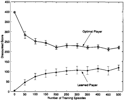
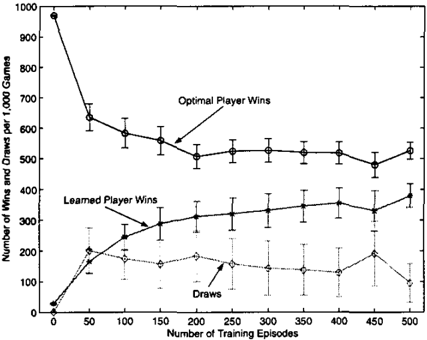
We conducted a series of experiments on a 4 x 4 grid to compare our learned player with the optimal minimax player (obtained by exact policy iteration) for this grid size. Training samples were collected by "random games", i.e., complete game trajectories where the players take random actions independently until scoring occurs. The average length of such a game in the 4 x 4 grid is about 60 steps. We varied the number of games from 0 to 500 in increments of 50. In all cases, our training sets had no more than 40, 000 samples. For each data set, LSPI was run until convergence or until a maximum of 25 iterations was reached. The final policy was compared against the optimal player in a tourna­ ment of 1, 000 games. A game was called a draw if scoring did not occur within 100 steps. The entire experiment was repeated 20 times and the results were averaged.

The results are summarized in Figures 1 -2, with error

9 There are actually 12 such positions, but two of them (the ones behind the attacker) are excluded because if the defender was there, P1 would be true.

bars indicating 95% confidence intervals. The player cor­ responding to 0 training episodes is a purely random player that selects actions with uniform probability. Clearly, LSPI finds better players with more training data. However, function approximation errors may prevent it from ulti­ mately reaching the performance of the optimal player.

We also applied our method to bigger soccer grids where obtaining the exact solution or even learning with a conven­ tional method is prohibitively expensive. For these grids, we used a larger set of basis functions (1400 total) that included several crossterms compared to the set described above. These terms were not included in the 4 x 4 case be­ cause of linear dependencies caused due to the small grid size. Below are listed the extra basis functions used in ad­ dition to the original ones listed above:

• P1 and not Pz
• (DHPAGv?. (SDvPAG?
• PAUG, PALG, PAWG
• P 1 and Pz
• (DHPAGv)2, (SDvPAG)2, PAWG
• SDHPAPD x SDvPAPv
• not P, and not Pz
• (DHPAGv)2, (SDvPAG)2, PAWG, SDvPAPv
• SDHPAPv x SDvPAPv,PvWG
• (SDvPAPv)2, (SDHPAPv)2
• not P, and Pz
• (DHPAGv)2, (SDvPAG)2, PAWG

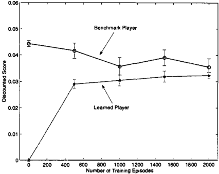
We obtained a benchmark player for an 8 x 8 grid by gener­ ating 2 samples, one for each ordering of player moves for each of the 201, 600 states and action combinations, and by using these artifically generated samples to do a uni­ form projection into the column space of <I?. In some sense, this benchmark player is the best player we could hope to achieve for the set of basis functions under consideration,

$1.8

三

一

assuming that uniform projection is the best one. Our anec­ dotal evaluation of this player is that it was very strong.

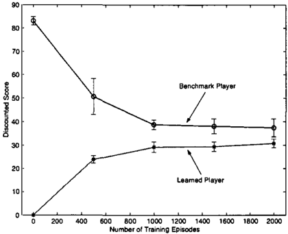
We conducted a series of experiments against learned play­ ers obtained using training sets of different sizes. Training samples were again collected by "random games" with a maximum length of 1, 000 steps. The average length was about 180 steps. We varied the number of such games from 0 to 2, 000 in increments of 500. In all cases, our train­ ing sets had no more than 400, 000 samples. For each data set, LSPI was run until convergence, typically about 8 iter­ ations. The final policy was compared against the bench­ mark player in a tournament of 1, 000 games. A game was called a draw if scoring had not occurred within 300 steps. Average results over 10 repetitions of the experiment are shown in Figure 3. Again, LSPI produces a strong player after a relatively small number of games.

To demonstrate generalization abilities we took all policies learned in the 8 x 8 grid and we tested them in a 40 x 40 grid. Our anecdotal evaluation of the benchmark player in the 40 x 40 grid was that played nearly as well as in the 8 x 8 grid. The learned policies also performed quite rea­ sonably and almost matched the performance of the bench­ mark player as shown in Figure 4. Note that we are com­ paring policies trained in the 8 x 8 grid. We never trained a player directly for the 40 x 40 grid since random walks in this domain would result mostly in random wandering with infrequent interaction between players or scoring, requiring a huge number of samples.

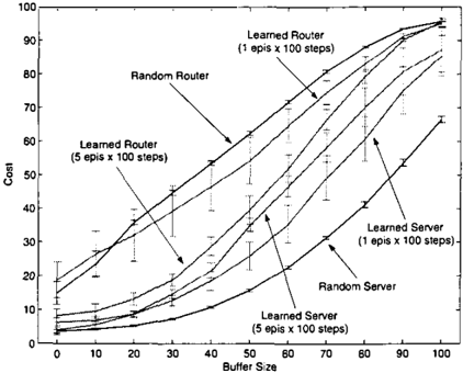
7.2 Flow Control

In the router/server flow control problem (Altman, 1994), a router is trying to control the flow of jobs into a server buffer under unknown, and possibly changing, service con­ ditions. This problem can be modeled as an MDP with the server being an uncertain part of the environment. How­ ever, to provide worst-case guarantees the router can view

the server as an opponent that plays against it. This view­ point enables to router to adopt control policies that per­ form well under worst-case/changing service conditions.

The state of the game is the current length of the buffer. The router can choose among two actions, low (L) and high (H), corresponding to a low (PAL) and a high (P AH) probability of a job arrival to the buffer at the current time step, with 0 < PAL < P AH � 1. Similarly, the server can choose among low (L) and high (H), corresponding to a low (PDL) and a high (PDH) probability of a job departure from the buffer at the current time step, with 0 � P D L < P D H < 1. Once the agents pick their ac­ tions, the size of the buffer is adjusted to a new state ac­ cording to the chosen probabilities and the game continues. The immediate cost R( s, a, o) for each transition depends on the current state s and the actions a and o of the agents:

where c( s) is a real non-decreasing convex function, a � 0, and {3 :0::: 0. c( s) is related to the holding cost per time step in the buffer, a is related to the reward for each in­ coming job, and {3 is related to the cost for the quality of service. The router attempts to minimize the expected dis­ counted cost, whereas the server strives to maximize it. The discount factor is set to 0.95.

Under these conditions, the optimal policies can be shown to have an interesting threshold structure, with mostly de­ terministic choices and randomization in at most one state (Altman, 1994). However, the exact thresholds and prob­ abilities cannot be easily determined analytically from the parameters of the problems which might actually be un­ known. These facts make the problem suitable for learning with function approximation. We used a polynomial of de­ gree 3 (1.0, s, s 2 , s3) as the basic block of basis functions to approximate the Q function for each pair of actions. That resulted in a total of 16 basis functions.

We tested our method on a buffer of length 100 with: PAL = 0.2, PAH = 0.9, PDL = 0.1, PDH = 0.8, c(s) = 10- 4 s 2 , a = -0.1, {3 = +1.5. With these set­ tings neither a full nor an empty buffer is desirable for ei­ ther player. Increasing the buffer size beyond 100 does not cause any change in the final policies, but will require more training data to cover the critical area (0-100).

Training samples were collected as random episodes of length 100 starting at random positions in the buffer. Fig­ ure 5 shows the performance of routers and servers learned using 0 (random player), 1, or 5 training episodes (the er­ ror bars represent the 95% confidence intervals). Routers are tested against the optimal server and servers are tested against the optimal router.10 Recall that the router tries to minimize cost whereas the server is trying to maxi­ mize. With about 100 or more training episodes the learned player is indistinguishable from the optimal player.

8 Conclusions and Future Work

We have demonstrated a framework for value function ap­ proximation in zero-sum Markov games and we have gen­ eralized error bounds from MDPs to the Markov game case, including a variation on the optimal stopping problem. A variety of approximate MDP algorithms can be general­ ized to the Markov game case and we have explored a generalization of the least squares policy iteration (LSPI) algorithm. This algorithm was used to find good policies for soccer games of varying sizes and was shown to have good generalization ability: policies trained on small soc­ cer grids could be applied successfully to larger grids. We also demonstrated good performance on a modest flow con­ trol problem.

10 The "optimal" behavior for this problem was determined by using a tabular representation and an approximate model obtained by generating 1000 next state samples for each Q-value.

One of the difficulties with large games is that it is diffi­ cult to define a gold standard for comparison since evalua­ tion requires an opponent, and optimal adversaries are not known for many domains. Nevertheless, we hope to attack larger problems in our future work, particularly the rich va­ riety of flow control problems that can be addressed with the Markov game framework. Queuing problems have been carefully studied and there should be many quite challeng­ ing heuristic adversaries available. We also plan to consider team-based games and general sum games.

Acknowledgements We are grateful to Carlos Guestrin and Michael Littman for helpful discussions. Michail G. Lagoudakis was partially supported by the Lilian Boudouri Foundation.

References

• Altman, E. (1994). Flow control using the theory of zero-sum markov games. IEEE Trans. on Auto. Control, 39,814-818.

Bertsekas, D., & Tsitsiklis, J. (1996). Neuro-dynamic program­ ming. Belmont, Massachusetts: Athena Scientific.

Bowling, M., & Veloso, M. (200 l ) . Rational and convergent learning in stochastic games. Proc. of /JCAI-0/.

Bradtke, S., & Barto, A. (1996). Linear least-squares algorithms for temporal difference learning. Machine Learning, 2, 33-58.

Gordon, G. J. (1995). Stable function approximation in dynamic programming. Proceedings of the Twelfth International Con­ ference on Machine Learning. Morgan Kaufmann.

Koller, D., & Parr, R. (2000). Policy iteration for factored MOPs. Proceedings of the Sixteenth Conference on Uncertainty in Ar­ tificial Intelligence (UAI-00). Morgan Kaufmann.

Lagoudakis, M., & Parr, R. (2001). Model free least squares pol­ icy iteration. To appear in 14th Neural Information Processing Systems (N/PS-/4).

Littman, M. L. (1994). Markov games as a framework for multi­ agent reinforcement learning. Proceedings of the I I th Inter­ national Conference on Machine Learning (ML-94). Morgan Kaufmann.

Solan, E., & Vieille, N. (2001). Quitting games. MOR: Mathe­ matics of Operations Research, 26.

Sutton, R. S. ( 1988). Learning to predict by the methods of tem­ poral differences. Machine Learning, 3 , 9-44.

Szepesvari, C., & Littman, M. ( 1999). A unified analysis of value-function-based reinforcement-learning algorithms. Neu­ ral Computation, I I, 2017-2059.

Van Roy, B. (1998). Learning and value function approxima­ tion in complex decision processes. Doctoral dissertation, Mas­ sachusetts Institute of Technology.

Williams, R. J., & Baird, L. C. I. (1993). Tight peiformance bounds on greedy policies based on impeifect value functions (Technical Report). College of Computer Science, Northeast­ em University, Boston, Massachusetts.