Vector-space Analysis of Belief-state Approximation for POMDPs

Pascal Poupart

Department of Computer Science University of Toronto Toronto, ON MSS 3H5 [email protected]

Abstract

We propose a new approach to value-directed be­ lief state approximation for POMDPs. The value­ directed model allows one to choose approxima­ tion methods for belief state monitoring that have a small impact on decision quality. Using a vec­ tor space analysis of the problem, we devise two new search procedures for selecting an approxi­ mation scheme that have much better computa­ tional properties than existing methods. Though these provide looser error bounds, we show em­ pirically that they have a similar impact on deci­ sion quality in practice, and run up to two orders of magnitude more quickly.

1 Introduction

Partially observable Markov decision processes (POMDPs) have attracted considerable attention as a model for decision-theoretic planning. Their generality allows one to seamlessly model sensor and action uncertainty, uncer­ tainty in the state of knowledge, and multiple objectives [ 1, 5]. Their computational intractability has, however, limited their practical applicability [ 11, 13].

An important approach to POMDPs involves constructing a value function for a belief state MDP offline, and maintain­ ing a belief state (or distribution over system states) online, which is used to implement an optimal policy [18]. Anum­ ber of approaches attacking the offline computational prob­ lems have been studied, including improved algorithms [6], the use of factored representations [2, 8], as well as numer­ ous approximation schemes [9]. Little work has focused on the online belief state monitoring problem. Because plan­ ning state spaces grow exponentially with the number of variables, maintaining an explicit distribution over states is generally impractical. Even when concise representa­ tions such as dynamic Bayes nets (DBNs) are used, moni­ toring is generally intractable, since the independencies ex­ ploited by DBNs vanish over time. Boyen and Koller [3] proposed projection schemes for approximate monitoring,

Craig Boutilier

Department of Computer Science University of Toronto Toronto, ON MSS 3H5 [email protected] essentially breaking weaker correlations among variables to ensure tractability. Poupart and Boutilier [15] proposed value-directed methods for approximation, allowing the an­ ticipated loss in expected utility guide the choice of approx­ imation scheme.

In this paper we pursue the value-directed approach since its emphasis on minimizing impact on decision quality is a critical factor in devising useful approximations. We use the value function itself to determine which correlations can be "safely" ignored when monitoring one's belief state. We propose an alternative approach to choosing approximation schemes for monitoring in POMDPs that overcomes many of the computational bottlenecks of [15]. We introduce a vector space formulation of the approximation problem that allows one to construct approximation schemes with looser error bounds, but much more quickly. Despite the looser bounds, we show empirically that decision quality is rarely worse than that obtained using the more intensive ap­ proaches. Our methods work in time roughly on order of the time taken to solve a POMDP, and since they run of­ fline, they can be used with any POMDP technique that can currently be applied. Furthermore, these methods take ad­ vantage of the factored (DBN) representations to avoid state enumeration. The offline cost allows much faster (approxi­ mate) online policy implementation. Even in cases where a POMDP must be solved in a traditional "flat" fashion, we typically have the luxury of compiling a value function offline. Thus, even for large POMDPs, we might reason­ ably expect to have value function information (either exact or approximate) available to direct the monitoring process. The fact that one is able to produce a value function offline does not imply the ability to monitor the process exactly in a timely online fashion.1 Finally, our model offers a novel view of the approximation problem for belief state monitor­ ing for POMDPs.

We briefly overview POMDPs and value-directed approx­ imation in Section 2. We present our vector space formu­ lation in Section 3 and provide some suggestive empirical

1 While techniques exist for generating finite-state controllers for POMDPs, there are still reasons for wanting to use value­ function-based approaches [14].

results in Section 4.

2 POMDPs and Belief State Monitoring

The key components of a POMDP are: a finite state space S; a finite action space A; a finite observation space Z; and a reward function R : S -+ R. Actions induce stochastic state transitions with specified probabilities, and an agent is provided with noisy observations of the system state (with specified probabilities). A reward is received at each state and an agent's objective is to control the system through ju­ dicious choice of action to maximize the expected reward obtained over some horizon of interest.

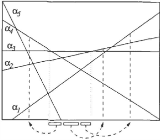
The rewards obtained over time by an agent adopting a spe­ cific course of action can be viewed as random variables R(t l. Our aim is to construct a policy that maximizes the ex­ pected sum of discounted rewards E{l::�o 'l R(t)) (where 1 is a discount factor less than one). An optimal course of action can be determined by considering the fully ob­ servable belief state MD P , where belief states (distributions over S) form states, and a policy 1r : B -+ A maps belief states into action choices. A key result of Sondik [18] showed that the value function V for a finite-horizon problem is piecewise-linear and convex and can be rep­ resented as a finite collection of a-vectors; for infinite­ horizon problems, a finite collection generally offers a good approximation. Specifically, one can generate a collection N of a-vectors, each of dimension lSI, such that V(b) :::;:: maxaEI:< b ·a. In Figure 1 the value function is given by the upper surface of the five vectors shown. Each vector is associated with a specific (course of) action. For finite horizon PO MOPs, a set N k is generated for each stage k of the process. Algorithms exist that construct efficient repre­ sentations of a-vectors, such as decision trees or algebraic decision diagrams (ADDs), when the POMDP is specified concisely using DBNs [2, 8].

Insight into the nature of PO MOP value functions can be gained by examining Monahan's [12] method for solving POMDPs. Monahan's algorithm proceeds by producing a sequence of k-stage-to-go value functions Vk, each repre­ sented by a set of a-vectors Nk. Each a E N k denotes the value (as a function of the belief state) of executing a k-step conditional plan. More precisely, let the k-step observation strategies be the set Oft of mappings u : Z -+ N k-1 . Then each a-vector in Nk corresponds to the value of ex­ ecuting some action a followed by implementing some u E OS'; that is, it is the value of doing a, and executing the k 1-step plan associated with the a-vector u(z) if z is observed. Using CP(a) to denote this plan, we have that CP(a) = (a;ifz;,CP(u(z;))'rlz;). We informally write this as (a; u). We write a ( (a; u)) to denote the a-vector re­ flecting the value of this plan.

The implementation of a policy requires that one monitor belief state b over time so that it may be "plugged" into the value function (or N) to make a suitable action choice. Be-

lief states can be maintained by standard Bayesian methods; but when lSI is large, the cost is prohibitive. This is espe­ cially true when S is determined by a set of variables X (and lSI :::: 0(2IXI)). In such cases, DBNs can be used to rep­ resent the dynamics ofPOMDPs and DBN inference tech­ niques that exploit conditional independence among vari­ ables can be applied to make monitoring more efficient. Un­ fortunately, as shown by Boyen and Koller [3}, in many problems most if not all variables of DBNs tend to become correlated over time so DBNs offer no significant savings.

Boyen and Koller introduced projection schemes as a method to approximate belief states. Given variables X defining S, a projection is a set S of subsets of X with each variable in at least one subset. Correlations among vari­ ables within a subset are preserved while the subsets are as­ sumed to be independent. For instance, if X:::;:: {A, B, C}, then projection S :::: { AB, C} approximates the exact be­ lief state b :::;:: Pr(A,B,C) with b' :::: Pr(AB)Pr(C). The assumed independence allows more efficient monitor­ ing using DBNs: at most, one maintains marginals over each subset inS.

The choice of projection scheme (or any other approx­ imation) can have a dramatic impact on decision qual­ ity in a PO MOP, since the approximate belief b' can lead to the choice of a suboptimal course of action. Poupart and Boutilier [15] propose a value-directed approximation framework allowing computation of bounds on the loss in expected utility for projection schemes, and search methods for choosing projections that tradeoff decision quality with monitoring efficiency. The techniques are computationally intensive (potentially requiring time quadratic in the solu­ tion time of the PO MOP); but this offline computation pro­ duces a projection scheme that improves online monitoring efficiency with minimal sacrifice in decision quality. We briefly outline this model.

Assume a PO MOP has been solved giving the set � of a­ vectors with a E N. Let R (a ) be the optimal region for a (i.e., the set of belief states b such that o: is maximal for b). Given a projection schemeS, the switch set Sw(a) is

the set of c/ such that S (b) E R(a') for some b E R(a). Thus, S could induce one to believe a ' has maximum value at the current belief state instead of a, thereby erroneously "switching to" the plan corresponding to a ' from a by using S. Figure 1 illustrates a switch set Sw( a3) = { a1, a2, a4 } . Switch sets can be computed by solving a nonlinear pro­ gram for each a EN. Linear programs (LPs) can be used to more effectively produce a superset of the switch set [15].

Given the switch sets (or supersets thereof), one can com­ pute an upper bound B� on the loss in expected value for a single approximation using S at k stages to go:

When multistage approximations are applied, one can de­ vise an alternative set which is similar in spirit to the switch set. The alternative set Alt ( a) is the set of all a-vectors cor­ responding to alternative plans that may be executed as a re­ sult of repeatedly approximating the belief state at all future time steps (see [15] for a precise definition). Alt ( a ) is con­ structed with a dynamic programming procedure similar to incremental pruning [ 6]. One can define an upper bound E� on the loss in expected value due to successive belief state approximations using S for k stages to go:

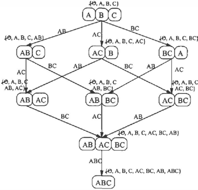
These bounds can be extended to infinite-horizon problems. Given the bounds B and E, one can search for an "opti­ mal" projection scheme by looking for the projection that minimizes one of those bounds. The space of projection schemes is very large (factorial in the number of variables), but exhibits a nice lattice structure. Figure 2 illustrates the lattice of projection schemes when the state space is defined by the joint instantiation of variables A, B and C. Each point denotes a projection scheme, with "descendents" of any projection corresponding to more coarse-grained pro­ jections. As we move down the lattice, accuracy increases since the number of correlations among the variables pre­ served in our belief state is increased (hence, error bounds B and E monotonically decrease); but monitoring effi­ ciency decreases as we move downward for the same rea­ son. A number of search procedures can be used to traverse the lattice, using the error bounds to guide the search. For example, a simple (and incremental) greedy scheme is pro­ posed in [15]. The search is stopped when a suitable accu­ racy/efficiency tradeoff has been reached.

3 Vector Space Analysis

We now provide a vector space analysis of belief state ap­ proximation by projection, showing in Section 3 .I that pro­ jections allow movement of belief state only in certain di­ rections (defining a subspace). This allows us to view a­ vectors as determining gradients of value in different direc­ tions: approximations whose directions give similar value gradients are less likely to cause switching (hence minimiz­ ing error). In Section 3.2 we use this to design faster switch

test algorithms than those described above, though yield­ ing looser bounds. In Section 3.3 we devise a new vector­ space search algorithm to find projections without directly trying to minimize these error bounds, instead relying on value gradient similarity.

3.1 Vector space formulation

Given a projectionS over X, let b and b' = S ( b ) be points in belief space. Define d = b' b to be the displacement vector from b to b'. Projection S determines a set of lin­ ear equations constraining b in terms of b'. For example, if X = {X, Y} and S = {X, Y} (i.e., S treats X, Y as independent), we have:

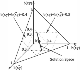
Geometrically, we interpret each equation as a hyperplane; and their intersection (or solution space) is a line through the origin representing a one-dimensional (in this example) subspace. This subspace captures the set of all displace­ ment vectors resulting from the application of S (w.r.t. b'). Since all possible displacement vectors lie on the same line, they must all have the same direction (vectors with opposite orientation are assumed to have the same direction).

To illustrate, let b(x) = 0.3 and b(y) = 0.4. The approxi­ mate belief state using S above gives:

Figure 3 shows a three-dimensional belief space for belief states xy, xy, xy and xy.2 All belief states b with b(x) =

2 We omit dimension b(xy) as probabilities sum to 1.

0.3lie in a hyperplane, and similarly for b(y) = 0.4. Their intersection is the set { b : b' = S (b)}, and all displace­ ment vectors forb' have the same direction. (For marginals other than 0.3 and 0.4, the hyperplanes and their intersec­ tion shift, but remain parallel).

Let Ds be the displacement subspace spanned by the set of all displacement vectors induced by S: it is completely characterized by its marginals (elements) and it describes the directions of all displacements. In general, Ds is a ( 2 1XI - c)-dimensional subspace, where c is the number of constraints, since it is the solution space of c linearly independent equations, each corresponding to a constraint d( m) = 0. ( c is the number of subsets of variables con­ tained in some subset m E S, as above.) This is obvious when we re\\rrite the constraints as Vm · d = 0, where Vm is a boolean lSI-vector with l at states with all X E m true and 0 at states with some X E m false.3 In our example, we have:

Let D� be t � e . subspace spanned by the vectors vm, m E S; the space D5 IS the null space of Ds (i.e., the set of vectors perpendicular to each vector in D s).

3.2 Vector space switch test

We will see below that the subspaces Ds and D� allow a nice characterization of a new switch test. We first con­ sider a simple relaxation of the switch test of [15]. Recall from Section 2 that approximation S could induce an agent to switch from optimal vector a i to suboptimal vector a j if S(b) E R(aj) for some bE R(o:i). The idea behind the re­ laxed vector space (VS) switch test is to simply apply the same technique ignoring the presence of other a-vectors. The VS switch test asks whether there is some belief state b for whichb·a; > b·ajyetS(b)·ai < S(b)·aj. If so,we say

3 The generalization to nonboolean variables is straightforward.

O:j is in the VS-switch set of a;. This is equivalent to ask­ ing if frj E Sw(a;) when all vectors except these two are removed from l{. Note that the VS-switch set is a superset of the true switch set.

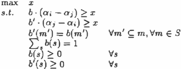
Since the constraints relating bandS( b) are nonlinear, VS­ switch sets can be computed using nonlinear programs. We can define a simpler linear VS-switch test as in Table 1 which produces a superset of the VS-switch set. This LP is a relaxation of the LP switch test [15}.

Now define frij = a, -aj to be a vector representing the difference in expected value for executing a j instead of a;. We can show that the VS-switch test for a; and O:j is pos­ itive iff a;j ¢ D"§. Consider a;j as a gradient that mea­ sures the error induced by an approximation when it causes a switch from a; to a j. After an approximation, if this dif­ ference changes considerably, the agent is likely to choose the wrong maximizing o:-vector. Define the relative error, O;j, of this change in the relative assessment of a; with re­ spect to O:j as:

Here a;j can be viewed as a gradient since approxima­ tions corresponding to displacement vectors d parallel to a;i maximize the magnitude of d · O:ij. In general, the an­ gle between d and a;j is a good indicator of approximation error. In particular, if they are perpendicular, their dot prod­ uct is zero and the relative assessment of a; and aj remains unchanged, preventing any switch. By definition, the sub­ space Df is the set of vectors perpendicular to all displace­ ment vectors possibly induced by S, so when aij is a mem­ ber of D"§, all possible displacement vectors are perpendic­ ular to a;j and consequently there cannot be a switch from a; to a j. Thus a;j ¢ D� iff the VS-switch test is positive. This fact provides for a much more efficient method to com­ ? ute switch sets than the LP of Table 1 . We decompose O:i j m two orthogonal vectors corresponding to the projections of a;j onto D� and D s:

(where proJ(a, D) stands for the projection of a onto D). If a;J E D�, then pro} ( a;i, D�) = a;J and, consequently, pro j (a;j, Ds) is the zero-vector; otherwise, proj(a;j,Ds) is nonzero. We can thus determine ifa;j E D-§ by measuring the length of pro j ( O:ij , D s). We have that IJproj(a;j, Ds) ll2 0 when a;i E D�, and ll p roj( a;j, Ds )ll2 > 0 when O:ij rf. D{ In particular, the squared length of proj(o:;j, Ds) can be computed by the following equation:

Here v-§ is some orthonormal basis spanning D-§. The spanning set of vectors Vm above can be used to generate several orthonormal bases using the Gram-Schmidt orthog­ onalization process and normalizing. We consider a spe­ cific orthonormal basis in particular-which we refer to as Vf-because of its factored representation. For problems involving binary variables, every vector in Vf consists of a sequence of 1 's and -1 's (before normalization). The un­ normalized basis vector iim associated with subset m has a 1 in every component corresponding to a state with an even number of true variables in m and -1 in every component corresponding to a state with an odd number of true vari­ ables in m. For instance, projection S = { XY, Y Z} has six marginals (0, X , Y, Z, XY andY Z), yielding the fol­ lowing basis vectors:4

With this orthonormal basis, we can implement VS-switch tests very effectively, without recourse to the LP in Table 1. We must simply compute Eq. 1 which requires O(c) dot products. If unstructured, each dot product requires 0 (IS I) elementary operations, for a total time ofO(ciSI). The use of factored representations such as ADDs considerably im­ proves this rwming time. Each basis vector has only two distinct values, and yields a very compact ADD representa­ tion. Assuming that the POMDP has been solved to pro­ duce ADD representations of the a-vectors, then the a;j will have compact representations, and the dot products will be computed very efficiently: often a small constant inde­ pendent of the size of the state space. Hence, for sufficiently structured POMDPs, the effective rwming time of a VS­ switch test is O(c).

By comparison, solving the linear program of an LP-switch test [ 15] is polynomial in the number of constraints c and the size of the state space. Furthermore, ADDs do not pro­ vide as useful a speed up for LPs since the effective state

4This definition can be generalized to non-binary variables.

space is the intersection of the abstract state space of all the constraints. The price paid is that the B and E bounds com­ puted using the VS-switch test will generally be looser than that using the original LP test. As in Section 2, these bounds can be used to search the lattice of projection schemes for making appropriate time-decision quality tradeoffs.

3.3 Vector space search

In this section we describe an alternative search method based on the relative error expression O;j. We do not com­ pute switch sets at all, nor attempt to minimize worst-case error bounds as above. This new vector-space (VS) search process instead seeks a projection S which defines a dis­ placement subspace D s that is as perpendicular as possible to all gradients O:ij. This is motivated by the observation that the more perpendicular the direction of an approxima­ tion with respect to a;j, the smaller the magnitude of J;j and, consequently, the less likely a switch will occur. Tech­ nically, this is done by minimizing the squared length of the projection of each gradient a;j on Ds (as in Eq. 1).

The length of pr o j ( a ; i, Ds) has a special interpretation: it corresponds to the greatest (absolute) relative error rate for an approximation in some direction d E Ds. The relative error rate corresponding to displacement vector dis the rel­ ative error induced by a unit displacement in the direction ofd:

Hence, by choosing a projectionS that minimizes Eq. 1, we are minimizing the (squared) worst relative error rate that may result from projection S. When ignoring the distance between the exact and approximate belief states, the rela­ tive error rate permits us to quantify how bad an approxi­ mation in some direction is likely to be. Each projection S constrains approximations to directions within the subspace Ds. The direction d E Ds with the highest (absolute) rel­ ative error rate has this worst relative error rate, which also happens to be ll pro j ( O:ij, Ds) ll2· Thus, it is desirable to try to minimize Expression 1.

Ideally we should choose an S that simultaneously mini­ mizes Eq. 1 for every gradient a;J (J i= i). In the absence of any prior information about the relative importance of each gradient, we suggest two simple schemes: (a) minimize the sum of squared lengths of each projection; or (b) minimize the squared length of the greatest projection:

We refer to these schemes as the sum and the max error es­ timators, respectively, for projection schemes. Of course, many other schemes could be proposed.

Given a vector o:; E �. VS search uses either Eq. 2 or Eq. 3 above to find a good projection S as follows. Starting at the root, we traverse the lattice of projection schemes (Fig­ ure 2) downward in a greedy manner. At each node, we pick the most promising child by minimizing Eq. 2 or Eq. 3 The computational complexity of a VS search is fairly low as it avoids LPs. Its running time is O(nc3J�I2ISI), since one good projection must be found for each of the I� I regions R(o:). For each region, O(nc2) nodes in the lattice are tra­ versed, each requiring the evaluation ofEq. 2 o r Eq. 3 which both take O(ci!XIISI) elementary operations.

The VS search can also be streamlined. The constraints of a node S are essentially the same as the constraints of its par­ ent node S' with one extra constraint corresponding to the marginal m that labels the edge connecting the two nodes. Since there is one basis vector per constraint, the following equation holds:

This means that both Eq. 2 and Eq. 3 can be computed in­ crementally as the lattice is traversed downward:

This incremental computation scheme for traversing the lat­ tice reduces the running time to O(nc2J�I2JSI) since only one dot product needs to be computed instead of one for each of the c constraints. This running time is significantly smaller thanO(nc2+ki�IISik) for the B-bound or E-bound greedy search with LP-switch tests used in [15]. As for the B-bound or E-bound greedy search with VS-switch tests, the running time O(nc3J�IJSI) is comparable. The VS search has an extra I � I factor, but one less c factor. In practice, I � I is usually larger than c, so the VS search is ac­ tually slower. Again, the upper bounds on running times are given in terms of lSI, but in practice, factored represen­ tations can drastically reduce the size of the effective state space for structured POMDPs.

4 Empirical Evaluation

Three test problems were used to carry out the experiments. The first POMDP is essentially the coffee problem intro­ duced by Boutilier and Poole [2]. The second POMDP is a variation of the widget problem described by Draper, Hanks

Table 2: Solution statistics for the three test problems

Problem	State Space Size		Size of !X		Solution
	full	effective	max	aver.	time (s)
Coffee	32	12	102	56	47
W i d g et	32	14	205	121	397
Pavement	128	85	39	16	250

and Weld [7]. The third POMDP is inspired from the pave­ ment maintenance problem described by Puterman [ 17]. Since the analysis of the experiments doesn't require any specific domain knowledge, the reader is referred to [14] in which the full specification of those problems is given.

Each of the three problems was solved using Hansen and Feng's [8] ADD implementation of incremental pruning (IP) to produce a set � of a-vectors using a compact ADD representation. Each problem is run to 15 stages (dis­ counted). Table 2 shows, for each problem, its full state space size, lSI, and i t s effective size, the largest intersec­ tion of abstract (ADD) states encountered during solution (specifically, the LP-dominance test in IP). The effective size is more relevant to solution time than jSj. We also show the solution time (in seconds) along with the average size of the sets !X over the fifteen stages and the maximum size set.

Once solved, we searched for a good projection scheme for each POMDP by minimizing different error bounds and/or using different switch tests, as described above. Specifi­ cally, six algorithms are tested: the B-bound and E-bound search of [15], which computes switch sets using an LP and chooses a projection using either the B or E error bounds; the VS analogs of these procedures which com­ putes weaker VS-switch sets using the algebraic formula­ tion of Section 3.2; and the VS search methods (sum and max) of Section 3.3, which ignore these bounds, but instead try to minimize Eq. 2 or Eq. 3. All search algorithms per­ form a lattice search within the set of projection schemes that partition variables in disjoint subsets. Furthermore, as­ suming that marginals of at most two variables provide a suitable efficiency/accuracy tradeoff, the lattice is traversed until all children of a node correspond to projections with a marginal with 3 variables. This last node is the projection scheme returned by the search.

We compare the time required to find a good projection us­ ing the different search procedures in Table 3. As expected, the running time is much less when using VS-switch tests (compared to LP-switch tests), since VS-switch tests do not require the solution of LPs. As for VS search algorithms, whether we minimize the sum of the relative error rates or their maximum, the running time is roughly the same and it is significantly faster than B-bound and E-bound search algorithms that use LP-switch tests, but a bit slower if VS

Table 3: Search running time in seconds

Problem	Solut. B-bd search			E-bds e a r ch		VS search
	time	LP	vs	LP	vs	max	sum
Coffee	47	1019	30	4379	2651	151	154
widget	397	1 0 1 4 2	109	89605	48695	707	703
Pavement	250	345	35	841	126	97	96

Table 4: Coffee problem: error comparisons

	Error	B-bd search		E-bd search		VS search
		LP	vs	LP	vs	max	sum
Single	Aver.	0.0013	0.0063	0.0063	0.0063	0.0013	0.0014
Approx	B-bd	3.2840	5.9150	4.3910	5.9150	3.2840	3.2840
Several	Aver.	0.0144	0.0161	0. 0 1 6 1	0 . 0 1 6 1	0.0154	0.0107
Approx	E-bd	13.085	13.085	13.085	13.085	13.085	13.085

switch tests are used forB-bound search. This is because, on the one hand, the VS search does not solve LPs (com­ pared to LP-switch tests), but on the other hand, it has a stronger dependence on the number of a-vectors (compared t o VS-switch te s t s ) . The time to search for good projections can be much worse than that of solving POMDPs (though this offline cost translates into online gains). In fact, only search procedures that avoid solving LPs scale effectively to larger problems. In some cases, these offer a decrease of up to two orders of magnitude. The running time ofVS pro­ cedures is roughly of the same order of magnitude as that of the POMDP solution procedures.

We also compare the actual average error, as well as the for­ mal B and E error bounds, obtained when applying the pro­ jection schemes found by various search algorithms (Tables 4, 5 and 6). The average error is the average loss incurred for 5000 random initial belief states generated from a uni­ form distribution. We see that the average error is essen­ tially the same whether the VS search procedure is used or some error bound is minimized. As a result, the dramatic computational savings associated with the VS procedures has effectively no impact on solution quality. Note that the B and E bounds are much larger than the average error observed because the bounds are concerned with the worst case scenario and, furthermore, they are not tight (supersets of the switch sets are really computed).

5 Concluding Remarks

We have proposed a new approach to value-directed belief state approximation for POMDPs. Our vector space approach-using either VS-switch tests or direct VS search-offers significant computational benefits over the value-directed methods proposed by Poupart and Boutilier [15]. While the error bounds are looser, we have seen in practice that our new schemes perform as well as the others

Table 5: Widget problem: error comparisons

	Error	B-bd search		E-bd search		VS search
		LP	vs	LP	vs	max	sum
Single	Aver.	0.0352	0 . 03 5 2	0.0352	0.0352	0.0082	0.0081
Approx	B-bd	3.4080	3.6270	3.4080	3.6270	3.4080	3.4080
Several	Aver.	0.0509	0.0508	0.0508	0.0508	0.0519	0.0517
Approx	E-bd	8.3811	8.3811	8.3811	8.3811	8.3811	8.3811

Table 6: Pavement problem: error comparisons

	Error	B-bd search		E-bd search		VS search
		LP	vs	LP	vs	max	sum
Single	Aver.	0.0015	0.0015	0.0015	0.0015	0.0014	0.0014
Approx	B-bd	5.3860	5.6900	5.3860	5.6900	5.3680	5.6160
Several	Aver.	0.0066	0.0066	0.0066	0.0066	0.0071	0.0028
Approx	E-bd	23.218	35.392	23.498	35.392	23.874	24.384

with respect to solution quality; thus the computational savings are achieved with little impact on decision quality. Furthermore, the vector space model provides new insights into the belief state approximation problem and how approximation impacts decision quality.

This novel view also gives us access to numerous tools from linear algebra to design approximation methods that could potentially offer better tradeoff's between decision quality and monitoring efficiency. For instance, it would be in­ teresting to investigate linear projectors since they allow the design of linear approximation methods by specifying (among other things) a displacement subspace Ds which could be made as perpendicular as possible to the gradi­ ent vectors aij. Linear projectors are well-studied approx­ imation methods with numerous properties and therefore they provide a promising alternative for improving value­ directed approximate belief state monitoring.

The success and scalability of our methods strongly de­ pends on the structure and compactness of the a-vectors. Therefore, one could also analyze the dependency between the a-vector structure and the conditional independence structure of the transition and observation functions. From a linear algebra perspective, the a-vectors can be viewed as a discounted sum of reward vectors multiplied by transition and observation matrices. Thus compact and structured a­ vectors could arise when the reward vectors fall into a small invariant subspace of the transition and observation matri­ ces. A possible direction of research would then be to re­ late the conditional independence structure of the transition and observation functions with their eigenvalue and eigen­ vector properties since they define the invariant subspaces. This would allow us to better characterize the situations in which our approach is suitable.

We are currently extending this approach, and its analysis,

in a number of different directions. First, we motivated this work by focusing on infinite-horizon POMDPs, though our algorithms and analysis assume a finite set of a-vectors. Of­ ten one is forced to approximate the value function (e.g., by producing a finite set of vectors where an infinite set is re­ quired, or simply by reducing the number of vectors to keep it manageable in size). Our algorithms can be applied di­ rectly to approximate value functions, and we expect that the analysis can be extended with suitable modifications as well. We are also interested in applying the idea of value­ directed monitoring to other representations of value func­ tions and other forms of approximate monitoring. The use of grid-based value functions [ 4, 9, 1 0] provides a very at­ tractive method for producing approximate value functions for which approximate monitoring will generally be neces­ sary. We expect that information in grid-based value func­ tions can be used profitably to direct the choice of projection (or other approximation) schemes. The use of value infor­ mation to guide other belief state approximation methods is also of tremendous interest: we have recently developed a sampling (particle filtering) algorithm that is influenced by value function information [ 1 6]. Finally, if it is taken for granted that some form ofbelief state approximation will be used, one might attempt to solve the POMDP to account for this fact; that is, can we construct policies that are optimal subject to the resource constraints placed on the monitoring process?

Acknowledgements: This research was supported by the Natural Sciences and Engineering Research Council and the Institute for Robotics and Intelligent Systems.

References

1. C. Boutilier, T. Dean, and S. Hanks. Decision theo­ retic planning: Structural assumptions and computa­ tional leverage. Journal of Artificial Intelligence Re­ search, 1 1: 1 -94, 1 999.
2. C. Boutilier and D. Poole. Computing optimal poli­ cies for partially observable decision processes using compact representations. In Proceedings of the Thir­ teenth National Conference on Artificial Intelligence, pages 1168-1175, Portland, OR, 1996.
3. X. Boyen and D. Koller. Tractable inference for com­ plex stochastic processes. In Proceedings of the Four­ teenth Conference on Uncertainty in Artificial Intelli­ gence, pages 33-42, Madison, WI, 1 998.
4. R. I. Brafman. A heuristic variable-grid solution method for POMDPs. In Proceedings of the Four­ teenth National Conference on Artificial Intelligence, pages 727-733, Providence, 1 997.
5. A. R. Cassandra, L. P. Kaelbling, and M. L. Littman. Acting optimally in partially observable stochastic do­ mains. In Proceedings of the Twelfth National Con­ ference on Artificial intelligence, pages 1023-1028, Seattle, 1994.
6. A. R. Cassandra, M. L. Littman, and N. L. Zhang. In­ cremental pruning: A simple, fast, exact method for POMDPs. In Proceedings of the Thirteenth Confer­ ence on Uncertainty in Artificial Intelligence, pages 54-61, Providence, RI, 1 997.
7. D. Draper, S. Hanks, and D. Weld. Probabilistic plan­ ning with information gathering and contingent exe­ cution. In Proceedings of the Second International Conference on AI Planning Systems, pages 31-36, Chicago, 1994.
8. E. A. Hansen and Z. F eng. Dynamic programming for POMDPs using a factored state representation. In P ro ­ ceedings of the Fifth International Conference on AI Planning Systems, Breckenridge, CO, 2000. 130- 139.
9. M. Hauskrecht. V a l uefu n ct i o n approximations for partially observable Markov decision processes. Journal of Artificial Intelligence Researr:h, 1 3:33-94, 2000.
10. [ 10] W. S. Lovejoy. A survey of algorithmic methods for partially observed Markov decision processes. Annals of Operations Researr:h, 28:47-66, 1991.
11. [ 1 1] 0. Madani, S. Hanks, and A. Condon. On the undecid­ ability of probabilistic planning and infinite-horizon partially observable Markov decision problems. In Proceedings of the Sixteenth National Conference on Artificial Intelligence, pages 541-548, Orlando, 1999.
12. [ 1 2] G. E. Monahan. A survey of partially observable Markov decision processes: Theory, models and algo­ rithms. Management Science, 28: 1- 1 6, 1982.
13. C. H. Papadimitriou and J. N. Tsitsiklis. The complex­ ity of Markov decision processes. Mathematics of Op­ erations Researr:h, 1 2(3):44 1-450, 1987.
14. [ 14] P. Poupart. Approximate value-directed belief state monitoring for partially observable Markov decision processes. Master's thesis, University of British Columbia, Vancouver, 2000.
15. [ 15] P. Poupart and C. Boutilier. Value-directed belief state approximation for POMDPs. In Proceedings of the Sixteenth Conf erence on Uncertainty in Artificial In­ telligence, pages 497-506, Stanford, 2000.
16. [16) P. Poupart, L. E. Ortiz, and C. Boutilier. Value­ directed sampling methods for monitoring POMDPs. In Proceedings of the Seventeenth Conference on Un­ certainty in Artificial Intelligence, Seattle, 2001. This volume.
17. [ 17] M. L. Puterman. Markov decision problems. Wiley, New York, 1 994.
18. [ 18] R. D. Smallwood and E. J. Sondik. The optimal con­ trol of partially observable Markov processes over a finite horizon. Operations Researr:h, 21:1071-1088, 1973.