Verbal Characterization of Probabilistic Clusters using Minimal Discriminative Propositions

Yoshitaka Kameya, Satoru Nakamura, Tatsuya Iwasaki /star and Taisuke Sato

Graduate School of Information Science and Engineering, Tokyo Institute of Technology 2-12-1 Ookayama, Meguro-ku, Tokyo 152-8552, Japan

Abstract. In a knowledge discovery process, interpretation and evaluation of the mined results are indispensable in practice. In the case of data clustering, however, it is often di ffi cult to see in what aspect each cluster has been formed. This paper proposes a method for automatic and objective characterization or 'verbalization' of the clusters obtained by mixture models, in which we collect conjunctions of propositions (attribute-value pairs) that help us interpret or evaluate the clusters. The proposed method provides us with a new, in-depth and consistent tool for cluster interpretation / evaluation, and works for various types of datasets including continuous attributes and missing values. Experimental results with a couple of standard datasets exhibit the utility of the proposed method, and the importance of the feedbacks from the interpretation / evaluation step.

1 Introduction

In a knowledge discovery process, interpretation and evaluation of the mined results are indispensable in practice. In the case of data clustering [1], however, it is often di ffi cult to see in what aspect each cluster has been formed, only from a list of the instances in the cluster. Visualization is a natural way for understanding things, and particularly in text clustering, Hotho et al. applied formal concept analysis with Hasse diagrams to visualize the similarity and dissimilarity among the obtained clusters [2]. On the other hand, since there would generally be a physical limitation or a high implementational cost in visualization, we would rather like to 'verbalize' the clusters, i.e. we associate an intuitive descriptive label (or a set of such labels) with each cluster. Additionally it seems desirable that the labels are chosen objectively and automatically from the clusters. So far, there have been only a few labeling methods, e.g. LabelSOM [3], Mei et al.'s automatic labeling for topic models [4] and others [5,6]. CLIQUE [7] also has a similar motivation to ours in that it performs hyper-rectangular clustering and at the same time produces comprehensible descriptions of the obtained clusters.

In this paper, we propose a new labeling method that associates conjunctions of propositions (attribute-value pairs), called propositional labels , with the clusters obtained by mixture models. For example, consider a cluster C which contains several creatures such as dolphins, mink, platypus and seals. Then, letting 'milk' and 'aquatic' be the boolean attributes of the creatures, (milk = True ∧ aquatic = True) would be a suitable propositional label for the cluster C , if none of the creatures in the other clusters has these properties together. Finally we easily find that C is a cluster of aquatic mammals. To find these propositional labels objectively and automatically, we conduct an Apriori-style breadth-first search for minimal propositional labels that discriminate the cluster of interest from the others. Due to these features, as we will see later, the proposed method can provide us with a new, in-depth and consistent tool for cluster interpretation / evaluation. It is also notable that, unlike the previous attempts, the proposed method is fully applicable to various types of datasets including continuous attributes and missing values. Another novel contribution of this paper is to show empirically the importance of the feedbacks from the interpretation / evaluation step in achieving a reasonable clustering result.

The rest of this paper is structured as follows. In Section 2, we describe the details of the proposed method. Section 3 then reports the experimental results with a couple of standard datasets. Finally, we mention the related work in Section 4, and conclude the paper in Section 5.

2 Proposed method

2.1 Preliminaries

Before starting, let us introduce some terminology and notation. Suppose that we have a dataset D of N instances which are described by m discrete attributes A 1 , A 2 , . . . , Am . Then, we simply refer to each instance by

/star Currently working at NTT Data Corporation

a = ( a 1 , a 2 , . . . , am ), where aj is a value of the j -th attribute Aj of the instance. Also we write V ( Aj ) as the set of possible values of Aj (i.e. aj ∈ V ( Aj ), 1 ≤ j ≤ m ). We now introduce a propositional label (or a label, for short) ' X 1 = x 1' ∧ ' X 2 = x 2' ∧· · · ∧ ' Xn = xn ' such that { X 1 , X 2 , . . . , Xn } ⊆ { A 1 , A 2 , . . . , Am } , Xi and Xi ′ are distinct ( i /nequal i ′ ), and xi ∈ V ( Xi ). In a probabilistic context, p (' X 1 = x 1' ∧ · · · ∧ ' Xn = xn ') = p ( X 1 = x 1 , . . . , Xn = xn ) holds. Also, p ( Z = z , . . . ) for a random discrete variable Z and its value z is generally abbreviated as p ( z , . . . ) if the context is clear.

Furthermore, we add some notational conventions. First, without loss of generality, we assume that the attribute values are not overlapped among attributes (i.e. V ( Aj ) ∩ V ( Aj ′ ) = ∅ for j /nequal j ′ ). Then, a propositional label ' X 1 = x 1' ∧ · · · ∧ ' Xn = xn ' is unambiguously simplified as x = ( x 1 ∧ · · · ∧ xn ) or x = ( x 1 , . . . , xn ). Here we have | x | = n , where | x | denotes the number of conjuncts in x , and is called the length of x . An instance a = ( a 1 , . . . , am ) is also regarded as a propositional label ' A 1 = a 1' ∧·· · ∧ ' Am = am '. In this paper, for notational brevity, we use a conjunctive form and a vector form for propositional labels interchangeably depending on the context. Besides, to simplify the algorithm descriptions presented later, in a propositional label ' X 1 = x 1' ∧·· · ∧ ' Xn = xn ', we will always enumerate X 1 , X 2 , . . . so that the order of enumeration preserves the original one A 1 , A 2 , . . . , i.e. for j 1 , j 2 , . . . jn such that Xi corresponds to Aji (1 ≤ i ≤ n , 1 ≤ j i ≤ m ), j i < j i ′ holds when i < i ′ .

Here consider a propositional label x = ( x 1 , . . . , xn ). Then, a label x ′ = ( x ′ 1 , . . . , x ′ n ′ ) is called a subconjunction of x if { x ′ 1 , . . . , x ′ n ′ } ⊆ { x 1 , . . . , xn } , and we denote this by x ′ ⊆ x . If x ′ ⊆ x but x ′ /nequal x , we write x ′ ⊂ x . For an instance a and a propositional label x , we say ' a satisfies x ' if x ⊆ a . For a boolean attribute Aj , we may abbreviate ' Aj = True' and ' Aj = False' as ' Aj = T' and ' Aj = F', respectively.

2.2 Overview

In this paper, we consider probabilistic clustering based on a simple mixture model called a naive Bayes model. A naive Bayes model has a latent class variable C taking on the identifiers { 1 , 2 , . . . , K } of K clusters, and represents a simple joint distribution: p ( C = k , A 1 = a 1 , . . . , Am = am ) = p ( C = k ) ∏ m j = 1 P ( Aj = aj | C = k ), or equivalently p ( k , a ) = p ( k ) ∏ j p ( aj | k ). Here the probabilities p ( k ) and p ( aj | k ) are treated as the model parameters. Given a dataset D of instances and the number K of clusters, we do:

1. Estimate the parameters in a model p ( k , a ) from D .
2. Assign the most probable class k ∗ ( a ) = argmax 1 ≤ k ≤ K p ( k | a ) to each instance a based on the estimated parameters. The k -th cluster C k is then formed as a set of instances a such that k ∗ ( a ) = k .
3. Find propositional labels x that characterize well each cluster C k .

In the first two steps, we perform clustering, and the third step is called labeling . As is well-known, the first step is realized by the EM (expectation-maximization) algorithm [8]. 1 From the second step, clustering can be casted as an unsupervised classification task, and we call p ( k | a ) the (class) membership probability of an instance a . In the last step, it is unspecified what are the propositional labels that characterize the clusters, and how to obtain them. The next two sections, Sections 2.3 and 2.4, address these issues, respectively.

2.3 Characteristic propositional labels

Relevance scores: To choose suitable propositional labels x = ( x 1 ∧ · · · ∧ xn ) or x = ( x 1 , . . . , xn ), of a cluster C k objectively and automatically, we introduce a scoring function that measures how relevant x and C k are. Previously, several relevance scores have been proposed in various statistical / data-mining tasks. The followings are an adaptation of those relevance scores to our labeling problem:

• -Growth rate: GR k ( x ) = p ( x | k ) / p ( x | ¬ k ), where ¬ k indicates that the instance under consideration belongs to a class other than k . This score is mainly used in emerging pattern mining [9] and explicitly states that the instances satisfying x are likely to occur in the cluster C k and unlikely to occur in the clusters other than C k . GR k ( x ) ranges from 0 (when p ( x | k ) = 0) to ∞ (when p ( x | k ) > 0 and p ( x | ¬ k ) = 0).
• -Membership probabilities: p ( k | x ). PRIM, a rule-based method for bump hunting, tries to find x such that p ( k | x ) ≥ r , where r is some threshold, under a separate-and-conquer strategy [10]. It is crucial to see that, for a fixed k , p ( k | x ) = p ( k ) p ( x | k ) / p ( x ) ∝ p ( x | k ) / p ( x ) holds. In class association rule (CAR) mining [11], p ( k | x ) is called the confidence of a rule x ⇒C k .

1 As discussed in Section 4, we can also use the K -means algorithm for clustering.

• -Pointwise mutual information: PMI k ( x ) = log p ( k , x ) -log { p ( k ) p ( x ) } . PMI has been used in text analysis [12]. This score is rewritten as log p ( x | k ) -log p ( x ), which is adopted by a well-known probabilistic clustering tool AutoClass [13] for post-analysis (named 'attribute influence values'), in a limited case with | x | = 1. The non-logarithmic version p ( k , x ) / ( p ( k ) p ( x )) is called the lift of a class association rule x ⇒C k [14].
• -Leverage: Leverage k ( x ) = p ( k , x ) -p ( k ) p ( x ). This score is often used for finding interesting association rules [15]. Leverage k ( x ) is equivalent to the weighted relative accuracy (WRAcc), a score used in subgroup discovery, and can be rewritten as p ( x )( p ( k | x ) -p ( k )) or p ( k ) p ( ¬ k )( p ( x | k ) -p ( x | ¬ k )) [16]. A related score | p ( x | k ) -p ( x | ¬ k ) | , often called support di ff erence , is used in contrast set mining [17].
• -TF-IDF: TF-IDF k ( x ) = p ( x | k ) log { 1 / p ( x ) } . This is a popular measure in information retrieval [18], and is a product of term frequency (TF) and inverse document frequency (IDF). TF of a term t in a document d is the relative frequency of t occurring in d , and IDF of t is the logarithm of the inverse of the relative frequency that a document containing t occurs in the whole document set. Then, assuming that a term occurs at most once in a document, the TF-IDF of a term t in a document d is given as p ( t | d ) log { 1 / p ( t ) } . Since TF-IDF is known to give a reasonably high score to t that characterizes d , TF-IDF k ( x ) above can be used by analogy where t corresponds to x , and d corresponds to k .
• -Precision / Recall: Precision and recall are also popular measures in information retrieval. In our context, p ( k | x ) and p ( x | k ) can be regarded as precision and recall of label x for the k -th cluster [14]. Also in COBWEB [19], a well-known conceptual clustering method, p ( k | x ) and p ( x | k ) are respectively used as metrics for inter-class dissimilarity and intra-class similarity. To balance the opposite behavior of precision and recall, in information retrieval, we often use thier harmonic mean 2 p ( k | x ) p ( x | k ) / ( p ( k | x ) + p ( x | k )) and call it the F-score . Lamirel et al. proposed the use of the F-score for automatic labeling of clustering results [6]. Similarly, the product of precision and recall p ( k | x ) p ( x | k ), which substantially works as the geometric mean of p ( k | x ) and p ( x | k ), is used by Popescul and Ungar [5].

Other relevance scores are discussed in comprehensive surveys by Kralj Novak et al. [16] and by Geng et al. [14]. It is easy to show that p ( k | x 1 ) ≤ p ( k | x 2 ) i ff GR k ( x 1 ) ≤ GR k ( x 2 ), 2 and p ( k | x 1 ) ≤ p ( k | x 2 ) i ff PMI k ( x 1 ) ≤ PMI k ( x 2). Consequently, for a particular cluster C k , the first three scores give the same ranking over the propositional labels. Hereafter we call p ( x | k ) the local support , and p ( x ) the global support . The relevance scores above commonly rely on the local support with a penalty regarding the global support. This contrastive use of the global support and the local support is also found in the category utility adopted in COBWEB [19].

In this paper, we choose p ( k | x ) as the relevance score for two reasons on intuitiveness for the end users. First, we can of course interpret p ( k | x ) as discriminative probabilities, by which we classify an instance satisfying x . As mentioned in Section 2.2, clustering is performed based on the membership probabilities p ( k | a ), which are a special case of p ( k | x ). The second reason is more practical: p ( k | x ) is inherently normalized (i.e. 0 ≤ p ( k | x ) ≤ 1). From this nature, we can use a threshold r , which just ranges over (0 , 1] and is commonly applied to all clusters, to filter out x such that p ( k | x ) < r .

Minimality: Let us consider two propositional labels x 1 and x 2 that fulfill some requirement (e.g. p ( k | x 1 ) ≥ r and p ( k | x 2 ) ≥ r for some threshold r ), and also suppose that x 1 ⊆ x 2 holds. In such a case, we favor x 1 over x 2 , because the longer one may have some redundant information which hinders us from understanding the cluster. In other words, we would like to have only minimal labels. In the literature on emerging pattern mining, such minimal patterns are called essential emerging patterns [20], and Ji et al. proposed an e ffi cient mining algorithm named ConSGapMiner for minimal distinguishing sequences [21].

Model-based computation of relevance scores: We have introduced several relevance scores which are based on probabilities. In most of the previous work, these probabilities are directly estimated from a given dataset D of instances. For example, membership probabilities are estimated as ˆ p ( k | x ) = |{ a ∈ C k | x ⊆ a }| / |{ a ∈ D | x ⊆ a }| . In our method, on the other hand, relevance scores are computed from the model parameters via the joint distribution (Section 2.2). This model-based approach has a couple of advantages. First, as seen later, we can e ffi ciently compute the scores, exploiting the conditional independence in the model, without scanning the whole dataset D . In many cases, the space for the model parameters is much smaller than the dataset. The second advantage is that the model parameters are well-abstracted data as long as the model fits to D , and there would be less chance to be a ff ected by noise. Finally, there is a positive side-e ff ect that we need not care about missing values in D since we only use the parameters estimated by the EM algorithm.

2 GR k ( x ) = ( p ( k ) / p ( ¬ k )) -1 ( p ( k | x ) / p ( ¬ k | x )) ∝ p ( k | x ) / (1 -p ( k | x )).

Selecting characteristic propositional labels: Now based on the discussions above, we define characteristic propositional labels , which characterize well the obtained clusters. A propositional label x of the cluster C k is characteristic i ff :

1. p ( k | x ) ≥ r ,
2. p ( x ) ≥ s global ,
3. p ( x | k ) ≥ s local, and
4. There is no x ′ ⊂ x that satisfies 1 ∼ 3 above,

where r , s global and s local are user-specified thresholds, and the probabilities p ( k | x ), p ( x ) and p ( x | k ) are computed via the joint distribution. Conditions 1 ∼ 4 are called the relevance condition , the global support condition , the local support condition , and the minimality condition , respectively.

While most of the existing CAR mining algorithms run based on the guide from the threshold for p ( x | k ), we treat the first and the fourth conditions as the primary filters. The remaining conditions are introduced to remedy the problem that we often obtain unintuitive characteristic labels with very low global / local support, and also to reduce the burden in the exhaustive search for characteristic labels, which will be described in the next section. So currently we do not consider to put a tight restriction on global / local support (e.g. s local = 1 / ( |D| / K ) = K / |D| , which implies that each of equally-sized clusters should contain at least one instance).

2.4 Exhaustive search for characteristic propositional labels

All possible propositional labels form a version space [22], and on this structure, we conduct an Apriori-style breadth-first search for the entire set of characteristic labels for each cluster. There are two major styles for such an exhaustive search: depth-first and breadth-first. We take a breadth-first style because, as seen later, it is easier to check the minimality of characteristic labels in a breadth-first style, 3 and because we do not necessarily need very long characteristic labels that are di ffi cult to read.

The F ind procedure (Algorithm 1) is the main routine of the search algorithm for characteristic labels, which calls the G en C andidate function (Algorithm 2). The basic flow is similar to Apriori (G en C andidate is our version of the apriori-gen function in [23]), but is di ff erent in that we make probability computation while generating candidates. In addition, since this probability computation requires normalization for each membership probability p ( k | x ), the most part of the algorithm should work in parallel for clusters. It is also crucial to note that the global / local support of x ( p ( x ) and p ( x | k )) are anti-monotonic w.r.t. the inclusion relation (i.e. p ( x | k ) ≥ p ( x ′ | k ) if x ⊆ x ′ ), but in general our relevance score is not. Instead, like ConSGapMiner , we make pruning based on the minimality of characteristic labels.

In the F ind procedure, for each C k , S n [ k ] indicates a set of propositional labels of length n that satisfy the global / local support condition, and Rn [ k ] indicates a set of labels in S n [ k ] that additionally satisfy the relevance condition. Rn [ k ] are the characteristic labels of length n which we wish to have, and we do not extend the labels in Rn [ k ]. Wn [ k ] = S n [ k ] \ Rn [ k ] are therefore the labels to be worked on next.

The candidate labels of length ( n + 1) are generated from the G en C andidate function, in which the labels of length n in Wn [ k ] are combined e ff ectively. In Line 5 of G en C andidate , like the 'prune' step of Apriori, 'S ub C onj ( x ext ) ⊆ Wn [ k ]' filters out the over-generated candidate labels using anti-monotonicity of global / local support and minimality at the same time. S ub C onj ( x ) is a function that returns a set of x 's subconjunctions of length | x | -1, 4 and using the property that Wn [ k ] = S n [ k ] \ Rn [ k ], the filtering condition requires that each of the immediate subconjunctions of x ext should be in S n [ k ] (due to anti-monotonicity), but should not be in Rn [ k ] (due to minimality). This way of filtering, together with the breadth-first strategy, enables us to perform e ff ective pruning by only checking the labels in Wn [ k ]. 5 Then, for each candidate label that has passed the filter, we compute the probabilities p ( x | k ), p ( x ) and p ( k | x ) (Lines 11-18). The point here is that we take the union of Cn + 1 [ k ]'s in advance (Line 11) to avoid a redundant computation, and reuse the previously computed values for p ( x prev | k ), exploiting the conditional independence in the naive Bayes model.

To speed-up further the search algorithm in the case with many attributes, in the F ind procedure, we optionally introduce a greedy pruning, similarly to a commercial data-mining tool named Magnum Opus [15]. To be more

3 ConSGapMiner mentioned above works in a depth-first fashion, and needs to introduce an extra data structure (a prefix tree) to reduce the time for the post-check on minimality.

4 More specifically, for x = ( x 1 , . . . , xn -1 , xn ), S ub C onj ( x ) = { ( x 2 , x 3 , . . . , xn -1 , xn ), ( x 1 , x 3 , . . . , xn -1 , xn ), . . . , ( x 1 , x 2 , . . . , xn -2 , xn ), ( x 1 , x 2 , . . . , xn -2 , xn -1 ) } .

5 Wn [ k ] is constructed from the labels in Wn -1 [ k ], and hence is guaranteed not to include any labels x such that x ′ ⊆ x , x ′ ∈ Rn ′ [ k ] and 1 ≤ n ′ ≤ n .

Algorithm 1 F ind

10: 11: 12: 13: 14: 15: 16: 17: 18:

1: for all k = 1 , 2 , . . . , K do 2: S 1 [ k ] : = { aj | 1 ≤ j ≤ m , aj ∈ V ( Aj ) , p ( aj ) ≥ s global , p ( aj | k ) ≥ s local } 3: R 1 [ k ] : = { aj ∈ S 1 [ k ] | p ( k | aj ) ≥ r } 4: W 1 [ k ] : = S 1 [ k ] \ R 1 [ k ] 5: end for 6: 7: n : = 1 8: while ∃ k : Wn [ k ] /nequal ∅ do 9: 〈 Cn + 1[1] , . . . , Cn + 1 [ K ] 〉 : = G en C andidate ( Wn [1] , . . . , Wn [ K ]) for all k = 1 , 2 , . . . , K such that Cn + 1 [ k ] /nequal ∅ do S n + 1 [ k ] : = { x ∈ Cn + 1 [ k ] | p ( x ) ≥ s global , p ( x | k ) ≥ s local } Rn + 1 [ k ] : = { x ∈ S n + 1 [ k ] | p ( k | x ) ≥ r } Wn + 1 [ k ] : = S n + 1 [ k ] \ Rn + 1 [ k ] end for n : = n + 1 end while return 〈 ⋃ n Rn [1] , . . . , ⋃ n Rn [ K ] 〉

concrete, we delete aj such that p ( k | aj ) < p ( k ) from S 1 [ k ] after Line 2. In addition, x = ( x 1 , . . . , xn , xn + 1 ) ∈ S n + 1 [ k ] such that p ( k | x ) < p ( k | x ′ ), where x ′ = ( x 1 , . . . , xn ), are considered as unpromising, and deleted from S n + 1 [ k ] after Line 11. This greedy pruning is unsafe, i.e. we may miss some characteristic labels actually satisfying the conditions in Section 2.3, but it would bring high e ffi ciency in many practical cases.

2.5 Handling continuous attributes

Until now, we have assumed that all attributes are discrete. To handle continuous attributes and discrete attributes consistently in terms of membership probabilities, we also 'propositionalize' each continuous attribute. To be more specific, as is often done in mixture modeling, we consider that each continuous attribute follows a univariate Gaussian distribution, in which two types of parameters, the mean µ j , k and the variance σ 2 j , k , are introduced for the j -th continuous attribute Aj and the k -th cluster C k . These parameters are also estimated by the EM algorithm. We further assume that we are given a set Q = { q 1 , q 2 , . . . , q |Q| } of di ff erent probabilities, where 0 < qh < 1 for 1 ≤ h ≤ |Q| , and the indices are given so that qh < qh ′ if h < h ′ . For instance, we may have Q = { 0 . 1 , 0 . 2 , . . . , 0 . 9 } . Then, using a cumulative distribution function Fj , k with the mean µ j , k and the variance σ 2 j , k for each Aj and C k , we introduce ' α ( j , k ) h < Aj ≤ β ( j , k ) h ' as a conjunct in a propositional label, where α ( j , k ) h = µ j , k -d ( j , k ) h and β ( j , k ) h = µ j , k + d ( j , k ) h such that Fj , k ( β ( j , k ) h ) -Fj , k ( α ( j , k ) h ) = qh . It can be seen here that α ( j , k ) h and β ( j , k ) h are symmetric w.r.t. the mean µ j , k . Hereafter we omit the superscript ( j , k ) unless they are needed.

Nowconsider x = ( x 0 ∧ ' α h < Xn ≤ β h ') and x ′ = ( x 0 ∧ ' α h ′ < Xn ≤ β h ′ ') where h < h ′ . Then, we define x ′ ⊂ x and we have p ( x ) < p ( x ′ ). With this new inclusion relation, in the search algorithm, an additional minimality check is made for the last conjunct corresponding to a continuous attribute, just after Rn [ k ] being computed. 6 One may see that α h 's and β h 's above are model-based quantile values, 7 and choosing an appropriate ' α h < Aj ≤ β h ' leads to an automatic adjustment of ( α h , β h ), which resembles the 'peeling' operation in PRIM, a rule-based bump hunting method [10].

3 Experiments

In the experiments, we used four datasets: the zoo dataset, the iris dataset, the 20 newsgroup dataset and the flags dataset. 8 For the first three datasets, we gave the correct number K of clusters to the clustering algorithm, considering ideal situations. We then compare the obtained characteristic labels and the original (human-annotated)

6 To be specific, after Lines 3 and 12 in the F ind procedure, non-minimal labels are deleted from both Rn [ k ] and S n [ k ].

7 For instance, if qh is given as 0.9, α h and β h respectively correspond to the 5%-tile value and the 95%-tile value under the Gaussian distribution.

8 The zoo dataset, the iris dataset and the flags dataset are available from the the UCI ML Repository ( http://archive.ics.uci.edu/ml/ ), and the 20 newsgroup dataset is available from the UCI KDD Archive ( http://kdd.ics.uci.edu/ ).

Algorithm 2 G en C andidate ( Wn [1] , . . . , Wn [ K ])

1: for all k = 1 , 2 , . . . , K do 2: Cn + 1 [ k ] : = ∅ 3: for all x = ( x 1 , . . . , xn -1 , xn ) ∈ Wn [ k ] and x ′ = ( x 1 , . . . , xn -1 , x ′ n ) ∈ Wn [ k ] such that ∀ j : xn , x ′ n /nelement V ( Aj ) do 4: x ext : = ( x 1 , . . . , xn -1 , xn , x ′ n ) 5: if S ub C onj ( x ext ) ⊆ Wn [ k ] then 6: Cn + 1 [ k ] : = Cn + 1 [ k ] ∪ { x ext } 7: end if 8: end for 9: end for 10: 11: Dn + 1 : = ⋃ K k = 1 Cn + 1 [ k ] 12: for all x = ( x 1 , . . . , xn -1 , xn , xn + 1 ) ∈ Dn + 1 do 13: x prev : = ( x 1 , . . . , xn ) 14: p ( x | k ) : = p ( x prev | k ) p ( xn + 1 | k ) for k = 1 , . . . , K 15: p ( x ) : = ∑ K k = 1 p ( k ) p ( x | k ) 16: end for 17: 18: p ( k | x ) : = p ( k ) p ( x | k ) / p ( x ) for k = 1 , . . . , K and x ∈ Cn + 1 [ k ] 19: 20: return 〈 Cn + 1[1] , . . . , Cn + 1 [ K ] 〉

classes. On the other hand, since the flags dataset does not contain the class information, we explore a plausible number of clusters by characteristic labels together with a Bayesian score for model selection. For simplicity, throughout the experiments, we set a small value (1 / |D| ) to the threshold s global for the global support p ( x ), so that the influence from s global is negligible. In addition, we tried 1,000 re-initializations in the EM algorithm not to get trapped into unwanted local optima.

3.1 Zoo dataset

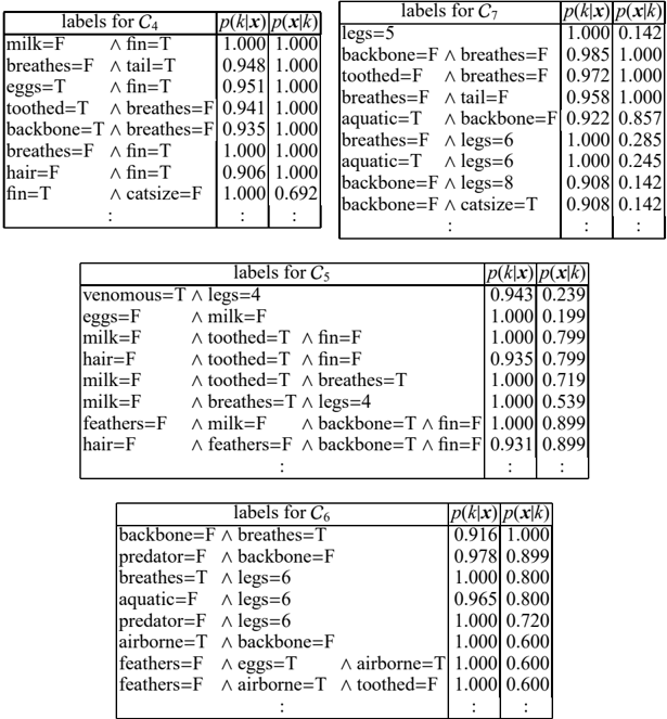
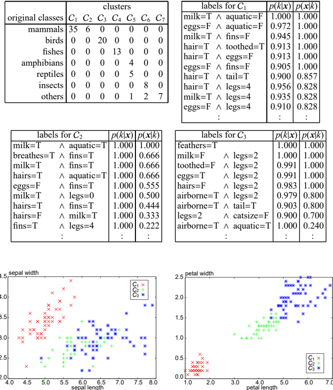
The zoo dataset describes the classification of 101 species of creatures with 17 attributes. The species are originally categorized into seven classes. Table 1 (top-left) shows the confusion matrix of the clustering result. We can see from this matrix that the creatures in the class 'mammals' are split into two clusters C 1 and C 2, whereas the creatures in 'reptiles' and 'amphibians' are merged into cluster C 5. Besides, the remaining tables in Table 1 show the obtained characteristic labels for C 1 , C 2 and C 3, where C 3 corresponds to the original class 'birds.' The labels in the tables are ordered firstly according to the length of x (i.e. syntactic generality), secondly according to the magnitude of p ( x | k ) (i.e. statistical generality), and thirdly according to the magnitude of p ( k | x ). 9 We used r = 0 . 9 and s local = K / |D| as the thresholds for p ( k | x ) and p ( x | k ), respectively, where D is the dataset and K = 3 is the number of clusters.

Since the original classes are unknown in real situations, we interpret the clusters C 1 , C 2 and C 3, only from the obtained characteristic labels. For example, all creatures in C 3 have feathers, so we can guess that C 3 corresponds to birds. Also there are several plausible labels for C 3 which support our guess. Interestingly, on the other hand, the obtained labels indicate that the (wrongly) split classes C 1 and C 2 correspond to terrestrial and aquatic mammals, respectively. So one may conclude that these split clusters are still meaningful. In the past, to evaluate the quality of the obtained clusters, there has been no way but to numerically check the closeness between the obtained clusters and the human-annotated classes, using some matching criteria, such as purity, normalized mutual information and the (adjusted) Rand index [18,24]. Contrastingly, as seen above, the characteristic labels provide us with a new and in-depth way for cluster evaluation. Similar interpretations are possible for the other clusters, whose characteristic labels are shown in Table 2.

3.2 Iris dataset

As a typical continuous dataset, we picked up the iris dataset, in which there are four attributes: petal width, petal length, sepal width and sepal length. Each of 150 cases in the dataset originally belongs to one of three classes: Setosa, Versicolour and Virginica. The confusion matrix and the obtained labels are shown in Table 3. We used

9 We also observed that intuitive labels tend to be highly ranked according to the harmonic mean of p ( k | x ) and p ( x | k ).

Table 1. The confusion matrix, and the characteristic labels for the clusters C 1 , C 2 and C 3 in the zoo dataset.

4.5

4.0

3.5

3.0

2.5

2.0

	clusters						labels for C 1 p ( k | x )				p ( x | k )
original classes	C 1	C 6	C 2 C 3	C 4 eggs	C 5 = F ∧	C 7		milk = T	∧ aquatic aquatic = F	= F 0.972	1.000	1.000	1.000
labels for C				p ( k | x ) p ( x | k )				labels for C 3		p ( k | x ) p ( x | k )
milk = T breathes = T milk = T hairs = T eggs = F milk = T hairs = T hairs = F fins = T	2 ∧ aquatic = T ∧ fins = T ∧ fins = T	1.000 0.666 1.000 0.555 1.000 0.500 1.000 0.444 1.000 0.333		1.000 1.000 1.000 0.666 1.000 0.666 eggs = T hairs = airborne airborne legs = 2	F = T = T		∧ ∧ ∧ ∧ ∧	feathers = T milk = F ∧ legs = 2 toothed = F ∧ legs = 2	legs = 2 legs = 2 legs = 2 tail = T catsize	1.000 1.000 1.000 1.000 0.991 1.000 0.991 1.000 0.983 1.000 0.979 0.800 0.903 0.800 = F 0.900 0.700 1.000 0.240
	∧ aquatic = T ∧ fins = T ∧ legs = 0 ∧ fins = T ∧ milk = T ∧ legs = 4 :			1 2 3 C C C				0.5 1.0 1.5 2.0 2.5 petal width		1 2 C C
3.5 4.0 4.5 sepal width								0.0		3 C
3.0
	5.5 6.0 6.5							2.0 3.0 4.0
				7.5 8.0				1.0		5.0 6.0
	sepal length
								:		7.0
								airborne = T ∧ aquatic = T
										: :
				: :
				1.000 0.222
				7.0
2.5
2.0
4.0 4.5 5.0
					length
				petal

the thresholds r = 0 . 9 and s local = K / |D| . A candidate set Q of cumulative probabilities (introduced in Section 2.5) is { 0 . 2 , 0 . 4 , 0 . 6 , 0 . 8 } . The scattered plots in Fig. 1 tell us that the obtained characteristic labels adaptively capture the dense part of cluster C 1. Also it should be noted that, in the proposed method, the Euclidean distance from the center of the cluster is translated into a cumulative probability under a Gaussian distribution.

3.3 20 newsgroups dataset

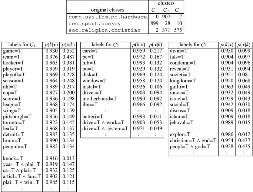
The 20 newsgroups dataset is originally a collection of approximately 20,000 articles from 20 di ff erent newsgroups. A preprocessed dataset available from http://people.csail.mit.edu/jrennie/20Newsgroups/ is used, and the articles from three newsgroups: comp.sys.ibm.pc.hardware , rec.sport.hockey and soc.religion.christian . We made further preprocessing: stemming by the Porter's algorithm [18], removing infrequent words ( ≤ 200 occurrences), removing short articles ( ≤ 10 words) and removing the attributes taking only one value. The dataset was finally converted into 2,799 bag-of-words boolean vectors whose dimension is 2,016. In labeling by the proposed method, we did not use the conjuncts of the form ' w = False' (or ' w = F')

labels for C 4		p ( k | x ) p (	x | k )
milk = F	∧ fin = T	1.000	1.000
breathes = F	∧ tail = T	0.948	1.000
eggs = T	∧ fin = T	0.951	1.000
toothed = T	∧ breathes = F	0.941	1.000
backbone = T	∧ breathes = F	0.935	1.000
breathes = F	∧ fin = T	1.000	1.000
hair = F	∧ fin = T	0.906	1.000
fin = T	∧ catsize = F	1.000	0.692
	:	:	:

labels for C 7		p ( k | x )	p ( x | k )
legs = 5		1.000	0.142
backbone = F	∧ breathes = F	0.985	1.000
toothed = F	∧ breathes = F	0.972	1.000
breathes = F	∧ tail = F	0.958	1.000
aquatic = T	∧ backbone = F	0.922	0.857
breathes = F	∧ legs = 6	1.000	0.285
aquatic = T	∧ legs = 6	1.000	0.245
backbone = F	∧ legs = 8	0.908	0.142
backbone = F	∧ catsize = T	0.908	0.142
:		:	:

labels for C 5			p ( k | x ) p ( x | k )
venomous = T ∧ legs = 4			0.943	0.239
eggs = F	∧ milk = F		1.000	0.199
milk = F	∧ toothed = T	∧ fin = F	1.000	0.799
hair = F	∧ toothed = T	∧ fin = F	0.935	0.799
milk = F	∧ toothed = T	∧ breathes = T	1.000	0.719
milk = F	∧ breathes = T ∧ legs = 4		1.000	0.539
feathers = F	∧ milk = F	∧ backbone = T ∧ fin = F	1.000	0.899
hair = F	∧ feathers = F	∧ backbone = T ∧ fin = F	0.931	0.899
:			:	:

labels for C 6		p ( k | x ) p ( x	| k )
backbone = F	∧ breathes = T	0.916	1.000
predator = F	∧ backbone = F	0.978	0.899
breathes = T	∧ legs = 6	1.000	0.800
aquatic = F	∧ legs = 6	0.965	0.800
predator = F	∧ legs = 6	1.000	0.720
airborne = T	∧ backbone = F	1.000	0.600
feathers = F	∧ eggs = T	1.000	0.600
feathers = F	∧ airborne = T	1.000	0.600
:		:	:

which means the absence of word w in the article. The thresholds r and s local were respectively configured as 0 . 9 and 10 × K / |D| . 10 Furthermore, we applied the greedy pruning described at the last of Section 2.4.

The results are shown in Table 4. From the obtained characteristic labels for C 1, it is seen that the article containing words such as 'hockei' ('hockey'; the su ffi x should have been replaced by the stemmer) and 'nhl' ('NHL'; the National Hockey League) are likely to belong to C 1. There are also the names of a hockey team and its home city (i.e. Pittsburgh Penguins). So we can guess from this information that C 1 is a cluster of articles related to hockey. Similarly, it is easy to see that C 2 is a cluster of articles related to computer hardware, 11 from the words such as 'mb' ('megabytes' or 'motherboard'), 'disk' and 'motherboard.' C 3 would be understood as a cluster that contains the articles talking about religious matters. Although there are many attributes in this dataset, our search algorithm is feasible, 12 thanks to the pruning based on the minimality and the optimized setting described above.

3.4 Flags dataset

The flags dataset contains the details of 194 national flags, originally described by 30 attributes. In this experiment, we focused on the clusters of national flags grouped on their visual aspects, and hence non-visual attributes (landmass, zone, area, population, language and religion) were removed in advance. As is written above, since

10 s local was configured as 10 × K / |D| because the 20 newsgroup dataset is 10 times (or more) larger than the zoo and the iris dataset.

11 As shown in the confusion matrix in Table 4, C 2 contains the articles from soc.religion.christian , but the characteristic labels related to religion did not appear. This would be because the articles from soc.religion.christian mainly use non-technical terms, which are less likely to form characteristic labels.

12 It took 404 seconds on a PC with Core i7 2.66GHz to get all characteristic labels for all clusters. Currently the search algorithm is implemented in the Ruby script language.

Table 3. (top) The confusion matrix in clustering the iris dataset, and (bottom) the obtained labels.

	clusters
original classes	C 1	C 2	C 3
Setosa	50	0	0
Versicolour	0	45	5
Virginica	0	0	50

labels for C 1 p ( k		| x )	p ( x | k )
0 . 06 < petal-w ≤ 0 . 43		0.999	0.800
1 . 2 < petal-l ≤ 1 . 7		1.000	0.799
3 . 3 < sepal-w ≤ 3 . 5		0.953	0.199
4 . 3 < sepal-l ≤ 5 . 6	∧ 3 . 0 < sepal-w ≤ 3 . 8	0.978	0.480
4 . 9 < sepal-l ≤ 5 . 1	∧ 2 . 8 < sepal-w ≤ 4 . 0	0.926	0.159

labels for C 2 p ( k | x )			p ( x | k )
4 . 0 < petal-l ≤ 4 . 4		0.931	0.799
5 . 5 < sepal-l ≤ 6 . 4	∧ 0 . 99 < petal-w ≤ 1 . 6	0.979	0.479
5 . 8 < sepal-l ≤ 6 . 0	∧ 2 . 6 < sepal-w ≤ 2 . 9	0.964	0.160

labels for C 3 p ( k | x )			p ( x | k )
4 . 5 < petal-l ≤ 6 . 4		0.985	0.800
6 . 4 < sepal-l ≤ 6 . 7		0.904	0.800
1 . 7 < petal-w ≤ 2 . 2		0.942	0.400
2 . 8 < sepal-w ≤ 3 . 1	∧ 1 . 6 < petal-w ≤ 2 . 4	0.918	0.480
2 . 8 < sepal-w ≤ 4 . 0	∧ 1 . 6 < petal-w ≤ 2 . 4	0.947	0.446

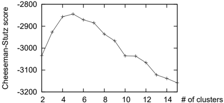
the class information is not given in this dataset, we first estimated the number of clusters as ˆ K by the CheesemanStutz score [13], a Bayesian model selection criterion adopted in AutoClass, and then starting from ˆ K , we explored a plausible number of clusters by observing the characteristic labels. Another point in this dataset is that discrete attributes and continuous attributes are mixed. That is, all of eight integer attributes (e.g. the number of circles in the flag) were treated as continuous attributes. We used r = 0 . 75 and s local = K / |D| as the thresholds for p ( k | x ) and p ( x | k ), respectively, where D is the dataset and K is the number of clusters. Also we conducted the greedy pruning.

Fig. 2 shows the curve of the Cheeseman-Stutz score with various numbers of clusters, and we have ˆ K = 5 as a peak of this curve. We further continued to compute characteristic labels with the number K of clusters being around ˆ K , and found that readable characteristic labels are obtained when K = 6. Table 5 presents these labels. 13 The shortest characteristic label for the cluster C 1 says that the national flags in C 1 (and none in the other clusters) have one saltire (diagonal cross). A typical example of such flags is the Union Jack, and actually many flags in C 1 have one quartered section (i.e. #quarters = 1) for the Union Jack. Similarly, the clusters C 2 and C 3 contain the flags with vertical bars and with circles, respectively. The label (#saltires = 0 ∧ #quarters = 1) for C 6 distinguishes C 1 and C 6, and similarly the labels (#crosses = 1 ∧ #saltires = 0) and (#crosses = 1 ∧ #quarters = 0) for C 4 jointly work for distinguishing C 4 from C 1 and C 6, where #crosses indicates the number of upright crosses. Indeed, C 6 contains the flag of the United States, and C 4 contains the flags of several Scandinavian countries (note that the Union Jack also contains upright crosses). From the labels for C 5, one may see that C 5 is a cluster of miscellaneous flags. On the other hand, when the number K of clusters is set at ˆ K = 5, the clusters C 2 and C 3 are merged into one cluster, whose characteristic labels are not so intuitive as in Table 5. These results imply that a plausible number of clusters can be determined by interactively consulting characteristic labels, with a help from model selection techniques, and clearly exemplify how the feedbacks from the interpretation / evaluation step contribute in knowledge discovery.

4 Related work

As mentioned above, there have been only a few labeling approaches. LabelSOM [3] is a labeling method for self-organizing maps, and Mei et al.'s automatic labeling method for unigram topic models [4] uses a heuristic score based on pointwise mutual information. As described in Section 2.3, di ff erent relevance measures are used

13 Since each continuous attribute Aj is originally an integer attribute, a proposition ' α < Aj ≤ β ' (assume here that α and β are not integers, for simplicity) was translated back into ' Aj = /ceilingleft α /ceilingright , /ceilingleft α /ceilingright + 1 , . . . , /floorleft β /floorright ' in Table 5. Non-minimal labels produced by this translation were then removed.

Table 4. The confusion matrix, and the characteristic labels for the clusters C 1 , C 2 and C 3 in the 20 newsgroups dataset.

	clusters
original classes	C 1	C 2	C 3
comp.sys.ibm.pc.hardware	0	907	7
rec.sport.hockey	899	28	10
soc.religion.christian	2	371	575

labels for C 1	p ( k | x )	p ( x | k )	labels for C 2	p ( k | x )	p ( x | k )	labels for C 3	p ( k | x )	p ( x | k )
game = T	0.930	0.552	card = T	0.959	0.217	divin = T	0.950	0.099
team = T	0.976	0.487	pc = T	0.972	0.167	fals = T	0.904	0.097
hockei = T	0.963	0.381	mb = T	0.993	0.132	condemn = T	0.904	0.096
player = T	0.959	0.319	bu = T	0.929	0.132	reveal = T	0.931	0.094
playo ff= T	0.969	0.278	disk = T	0.969	0.124	societi = T	0.921	0.081
season = T	0.964	0.248	window = T	0.958	0.124	kingdom = T	0.920	0.068
nhl = T	0.989	0.217	instal = T	0.926	0.106	guilti = T	0.963	0.049
cup = T	0.927	0.200	driver = T	0.903	0.094	innoc = T	0.932	0.049
score = T	0.936	0.198	motherboard = T	0.990	0.092	israel = T	0.959	0.043
leagu = T	0.968	0.174	ibm = T	0.966	0.092	social = T	0.942	0.030
wing = T	0.905	0.159	:	:	:	diseas = T	0.909	0.018
pittsburgh = T	0.956	0.149	batteri = T	0.993	0.011	islam = T	0.909	0.018
toronto = T	0.922	0.145	drive = T ∧ work = T	0.903	0.053	jehovah = T	0.989	0.015
leaf = T	0.968	0.137	drive = T ∧ system = T	0.971	0.049	:	:	:
detroit = T	0.983	0.135	:	:	:	explor = T	0.986	0.012
bruin = T	0.990	0.134				christian = T ∧ god = T	0.954	0.437
penguin = T	0.982	0.134				peopl = T ∧ god = T	0.928	0.435
:	:	:				:	:	:
knock = T	0.916	0.013
year = T ∧ plai = T	0.919	0.147
ca = T ∧ plai = T	0.932	0.125
articl = T ∧ fan = T	0.902	0.121
plai = T ∧ win = T	0.985	0.115
:	:	:

by Popescul and Ungar [5] and by Lamirel et al. [6] for automatic labeling of document clusters. In these labeling methods, the length of possible labels seems to be limited in advance, and thus no pruning mechanism, like the one described in Section 2.4, is given.

CLIQUE [7] is a novel hyper-rectangular clustering method that additionally gives comprehensible descriptions of the obtained clusters. The description of each cluster is a DNF formula of the ranges of continuous attributes such as ((30 ≤ age < 50) ∧ (4 ≤ salary < 8)) ∨ ((40 ≤ age < 60) ∧ (2 ≤ salary < 6)). Although CLIQUE has a similar motivation to ours, it is mainly designed for the dataset with continuous attributes. According to the original description ('Remarks' in Section 2.2 of [7]), if we use discrete attributes, all instances in a cluster must take the same value for each discrete attribute in a selected subspace. In the proposed method, contrastingly, we do not have such a restriction, and as seen in Section 3.4, we can make use of advanced statistical techniques such as ones for model selection in the clustering step. The latter point also contrasts the proposed method with conceptual clustering methods such as COBWEB [19].

In the research on expert systems, it has been a problem to explain the expert system's conclusion to human users. Wolverton [25] proposed the use of satisficing conclusion-substantiating (SCS) explanations to explain an expert system's conclusion. Given a system's conclusion c and a threshold ρ , the SCS explanation e is the shortest sequence of facts such that p ( c | e ) > ρ (or if no such sequence of facts, e = argmax e ′ p ( c | e ′ )). Our search algorithm would contribute in e ffi cient finding of SCS explanations.

Traditional rule induction methods such as C4.5 and RIPPER [26] can also be applied to find comprehensible cluster descriptions. However, Hotho et al. reported that these methods tend to produce too many rules to manage for human [2]. One possible reason is that C4.5 and RIPPER have a representational limitation that the premises in the obtained rules are always exclusive and need to be understood fragmentarily. In the proposed method, on the other hand, each characteristic label is independently interpretable. Another possibility is that C4.5 and RIPPER tried to find the exact boundaries among clusters, by their design. In labeling, however, we do not always

Table 5. The characteristic labels for C 1 , . . . , C 6 in the flags dataset.

labels for C 1	p ( k | x )	p ( x | k )
#saltires = 1	1.000	0.900	labels for C 4	p ( k | x )	p ( x | k )
topleft = white ∧ #quarters = 1	0.817	0.622	#crosses = 1 ∧ #saltires = 0	0.810	0.81003
stripes = 0,1,2 ∧ #quarters = 1	0.827	0.540	#crosses = 1 ∧ #quarters = 0	0.829	0.81002
botright = blue ∧ #quarters = 1	0.819	0.505	#crosses = 1 ∧ #sunstars = 0	0.751	0.720
green = T ∧ #crosses = 1	0.906	0.467	#circles = 0 ∧ #crosses = 1	0.768	0.640
gold = T ∧ #crosses = 1	0.763	0.467	green = F ∧ #crosses = 1	0.757	0.500
mainhue = blue ∧ #quarters = 1	0.810	0.467	#colors = 2,3 ∧ #crosses = 1	0.759	0.490
#crosses = 1 ∧ #quarters = 1	0.751	0.420	gold = F ∧ #crosses = 1	0.754	0.356
:	:	:
			labels for C 5	p ( k | x )	p ( x | k )
labels for C 2	p ( k | x )	p ( x | k )	#bars = 0	0.803	0.900
#bars = 1,2,3,4	0.782	0.800	#circles = 0	0.752	0.900
			#crosses = 0	0.755	0.600
labels for C 3	p ( k | x )	p ( x | k )	#quarters = 0	0.752	0.400
#circles = 1,2 ∧ #crosses = 0	0.781	0.540	triangle = T	0.889	0.240
#circles = 1,2 ∧ #quarters = 0	0.781	0.540	botright = black	0.888	0.080
black = T ∧ #circles = 1	0.766	0.225	mainhue = black	0.799	0.040
blue = F ∧ #circles = 1	0.765	0.200	:	:	:
botright = green ∧ #circles = 1,2	0.781		0.181
topleft = orange ∧ #saltires = 0	0.999	0.135	labels for C 6	p ( k | x )	p ( x | k )
topleft = orange ∧ #crosses = 0	0.970	0.135	#saltires = 0 ∧ #quarters = 1	0.960	0.360
mainhue = orange ∧ #crosses = 0	0.970	0.135	topleft = blue ∧ #quarters = 1	0.875	0.320
:	:	:

have to find such exact boundaries. Furthermore, traditional rule induction methods often su ff er from a so-called rare-class problem [27] when we have imbalanced or many clusters (if there are many clusters, each cluster is relatively rare). For example, small groups of instances (small disjuncts) in a rare class are often missed. Actually, in the zoo dataset, C4.5 / RIPPER only generated the rules for the cluster C 3 ('birds'): 'feathers = True' ⇒ C 3 , and 'feathers = False' ⇒ ¬C 3, and the rest of the antecedent patterns we found (Table 1, bottom-right) were ignored. This is presumably because most of the instances have been covered by the simple rules above in the rule construction process of C4.5 / RIPPER. It is reported that a classifier based on emerging patterns works well for the rare-class problem [28].

Recently it is proposed in [16] to unify three similar data mining tasks, contrast set mining, emerging pattern mining and subgroup discovery, under the name of supervised descriptive rule discovery . Our labeling method can be seen as a model-based approach in this framework, which focuses on interpretation / evaluation of probabilistic clusters. In a broader context, for knowledge discovery under an unsupervised setting, a sequential run of clustering and discriminative labeling would be a promising alternative to frequent pattern mining. Besides, also recently, Zimmermann and De Raedt introduced a general data mining task called cluster-grouping [29], and a branch-and-bound algorithm, named CG, for this task. CG e ffi ciently finds characteristic patterns (labels, in our case) following a guide from a convex relevance score such as χ 2 , information gain (used in ID3), WRAcc (Section 2.3) and category utility (used in COBWEB). Although this algorithm is powerful, it could not be directly applied to our labeling problem, since the membership probability p ( k | x ) seems not convex.

In the context of probabilistic modeling, the proposed method with mixture models could be extended for evidence-based sensitivity analysis (e.g. [30]) or explanatory analysis (e.g. [31]) of Bayesian networks, in which the membership probability p ( k | x ) is generalized as p ( q | e ), where q is an instantiation of a query variable and e is an instantiation of (a part of) evidence variables, and thus we search for a minimal combination e of evidences which is highly influential to the observation q . To the best of our knowledge, the most recent and closest work is Yuan et al.'s general framework for most relevant explanation (MRE) [32,33]. Their MRE framework adopts a relevance score called generalized Bayes factor (GBF), defined as GBF k ( x ) = p ( k | x ) / p ( k | ¬ x ) in our labeling problem. The MRE framework looks attractive, but seems unfit to our case for a couple of reasons. First, for the k -th cluster, a ranking over the propositional labels x by GBF k ( x ) is di ff erent from the one used in the clustering step (i.e. by p ( k | x )). Second, GBF k ( x ) = 1 -p ( x ) 1 -p ( x | k ) · p ( x | k ) p ( x ) can be numerically unstable when p ( x | k ) ≈ 1. For instance, we cannot order the labels x such that p ( x | k ) = 1, which in fact appear in one of our experiments (i.e. Table 1). Third, the MRE framework only provides an MCMC-based approximate method or an exact (exhaustive) method without safe pruning (like the one based on global / local support and minimality in the proposed method) for finding relevant x . Lastly, the MRE papers do not describe how to handle continuous attributes.

Handling continuous attributes is an important issue in CAR (class association rule) mining. For example, Washio et al. [34] proposed a CAR mining method that discretizes the continuous space on the fly with hyperrectangular clustering. The di ff erence from our labeling method is that we are given probabilistic clusters from beginning and thus we e ff ectively limit propositions to the ones of the form ' α < Aj ≤ β ', where α and β are symmetric w.r.t. the mean in the cluster. Besides, as in usual CAR mining, Washio et al.'s method searches for the antecedent patterns x based on the local support p ( x | k ).

Section 2.2 described that the EM algorithm is adopted for clustering. We can also use the K -means algorithm instead, since K -means can be seen as an instance of a parameter estimation framework often called Viterbi training , 14 tailored for a Gaussian mixture model with equal class probabilities and a common covariance matrix of the form σ 2 I [35]. Once the model parameters have been estimated, our labeling method is applicable as written in this paper. Similarly to the case in Section 3.2, when combined with K -means, the Euclidean distance from the centroid (the mean in the cluster) is translated into a cumulative probability under a Gaussian distribution.

5 Conclusion and future work

In this paper, we proposed a new labeling method that associates propositional labels (conjunctions of attributevalue pairs) with the clusters obtained by mixture models, to help us interpret or evaluate the clusters. As shown in the experimental results, the proposed method finds a set of intuitive descriptive labels that characterize well or 'verbalize' the clusters. The proposed method is fully applicable to various datasets including continuous attributes and missing values, and can be a new, in-depth and consistent tool for cluster interpretation / evaluation. Besides, the experimental results also show that the feedbacks from the interpretation / evaluation step can play an important role for achieving a reasonable clustering result. In future work, we would like to extend the proposed method to use disjunctive formulas or a richer representation. For example, we may merge two similar characteristic labels (milk = T ∧ legs = 4) and (hair = T ∧ legs = 4) into ((milk = T ∨ hair = T) ∧ legs = 4) to gain a higher local support. In a purely logical sense, our labeling algorithm can be formulated under the setting of inductive logic programming (ILP) with a simple refinement operator. As in ILP, the use of background knowledge such as taxonomy seems helpful for having more comprehensible descriptions.

Acknowledgments.

The authors would like to thank Toshihiro Kamishima for his helpful comments on related work. This work is supported in part by Grant-in-Aid for Scientific Research (No. 20240016) from Ministry of Education, Culture, Sports, Science and Technology of Japan.

References

1. Jain, A.K., Murty, M.N., Flynn, P.J.: Data clustering: a review. ACM Computing Surveys 31 (3) (1999) 264-323
2. Hotho, A., Staab, S., Stumme, G.: Explaining text clustering results using semantic structures. In: Proc. of the 7th European Conf. on Principles and Practice of Knowledge Discovery in Databases (PKDD-03). (2003)

14 Viterbi training has also been called hard EM, Viterbi EM, classification EM, sparse EM, and so on.

1. Rauber, A.: LabelSOM: on the labeling of self-organizing maps. In: Proc. of the 1999 Int'l Joint Conf. on Neural Networks (IJCNN-99). (1999) 3527-3532
2. Mei, Q., Shen, X., Zhai, C.: Automatic labeling of multinomial topic models. In: Proc. of the 13th ACM SIGKDD Int'l Conf. on Knowledge Discovery and Data Mining (KDD-07). (2007) 490-499
3. Popescul, A., Ungar, L.H.: Automatic labeling of document clusters. Unpublished manuscript available from http:// www.cis.upenn.edu/˜popescul/ (2000)
4. Lamirel, J.C., Ta, A.P., Attik, M.: Novel labeling strategies for hierachical representation of multidimensional data analysis results. In: Proc. of the 26th IASTED Int'l Conf. on Artificial Intelligence and Applications (AIA-08). (2008) 169-174
5. Agrawal, R., Gehrke, J., Gunopulos, D., Raghavan, P.: Automatic subspace clustering of high dimensional data for data mining applications. In: Proc. of the 1998 ACM SIGMOD Int'l Conf. on Management of Data (SIGMOD-98). (1998) 94-105
6. Dempster, A.P., Laird, N.M., Rubin, D.B.: Maximum likelihood from incomplete data via the EM algorithm. J. of the Royal Statistical Society B39 (1977) 1-38
7. Dong, G., Li, J.: E ffi cient mining of emerging patterns: discovering trends and di ff erences. In: Proc. of the 5th ACM SIGKDD Int'l Conf. on Knowledge Discovery and Data Mining (KDD-99). (1999) 43-52
8. Friedman, J.H., Fisher, N.I.: Bump hunting in high-dimensional data. Statistics and Computing 9 (1999) 123-143
9. Liu, B., Hsu, W., Ma, Y.: Integrating classification and association rule mining. In: Proc. of the 4th ACM SIGKDD Int'l Conf. on Knowledge Discovery and Data Mining (KDD-98). (1998) 80-86
10. Church, K.W., Hanks, P.: Word association norms, mutual information, and lexicography. In: Proc. of the 27th Annual Meeting on Association for Computational Linguistics (ACL-89). (1989) 76-83
11. Cheeseman, P., Stutz, J.: Bayesian classification (AutoClass): theory and results. In: Advances in Knowledge Discovery and Data Mining. The MIT Press (1995)
12. Geng, L., Hamilton, H.J.: Interestingness measures for data mining: a survey. ACM Computing Surveys 38 (3) (2006) 1-32
13. Webb, G.I., Butler, S., Newlands, D.: On detecting di ff erences between groups. In: Proc. of the 9th ACM SIGKDD Int'l Conf. on Knowledge Discovery and Data Mining (KDD-03). (2003) 256-265
14. Kralj Novak, P., Lavraˇ c, N., Webb, G.I.: Supervised descriptive rule discovery: a unifying survey of contrast set, emerging pattern and subgroup mining. J. of Machine Learning Research 10 (2009) 377-403
15. Bay, S.D., Pazzani, M.J.: Detecting group di ff erences: mining contrast sets. Data Mining and Knowledge Discovery 5 (2001) 213-246
16. Manning, C., Raghavan, P., Sh¨ utze, H.: Introduction toInformation Retrieval. Cambridge Univ. Press (2008)
17. Fisher, D.: Knowledge acquisition via incremental conceptual clustering. Machine Learning 2 (1987) 139-172
18. Fan, H., Ramamohanarao, K.: A Bayesian approach to use emerging patterns for classification. In: Proc. of the 14th Australasian Database Conf. (ADC-03). (2003) 39-48
19. Ji, X., Bailey, J., Dong, G.: Mining minimal distinguishing subsequence patterns with gap constraints. Knowledge and Information Systems 11 (3) (2007) 259-286
20. Mitchell, T.: Machine Learning. McGraw-Hill (1997)
21. Agrawal, R., Srikant, R.: Fast algorithms for mining association rules in large databases. In: Proc. of the 20th Conf. on Very Large Data Bases (VLDB-94). (1994) 487-499
22. Meil˘ a, M.: Comparing clusterings - an information based distance. J. of Multivariate Analysis 98 (2007) 873-895
23. Wolverton, M.: Presenting significant information in expert systems explanation. In: Proc. of the 7th Portuguese Conf. on Artificial Intelligence. (1995) 435-438
24. Witten, I.H., Frank, E.: Data Mining: Practical Machine Learning Tools and Techniques. 2nd edn. Morgan Kaufmann (2005)
25. Weiss, G.M.: Mining with rarity: a unifying framework. ACM SIGKDD Explorations 6 (1) (2004) 7-19
26. Ramamohanarao, K., Bailey, J., Fan, H.: E ffi cient mining of contrast patterns and their applications to classification. In: Proc. of the 3rd Int'l Conf. on Intelligent Sensing and Information Processing (ICISIP-05). (2005) 39-47
27. Zimmermann, A., De Raedt, L.: Cluster grouping: from subgroup discovery to clustering. Machine Learning 77 (2009) 125-159
28. Jensen, F.V.: An Introduction to Bayesian Networks. UCL Press (1996)
29. Chajewska, U., Halpern, J.Y.: Defining explanation in probabilistic systems. In: Proc. of the 13th Conf. on Uncertainty in Artificial Intelligence (UAI-97). (1997) 62-71
30. Yuan, C., Lu, T.C.: A general framework for generating mutlivariate explanations in Bayesian networks. In: Proc. of the 23rd AAAI Conf. on Artificial Intelligence (AAAI-08). (2008) 1119-1124
31. Yuan, C., Liu, X., Lu, T.C., Lim, H.: Most relevant explanation: properties, algorithms, and evaluations. In: Proc. of the 25th Conf. on Uncertainty in Artificial Intelligence (UAI-09). (2009) 631-638
32. Washio, T., Nakanishi, K., Motoda, H.: A classification method based on subspace clustering and association rules. New Generation Computing 25 (2007) 235-245
33. Celeux, G., Govaert, G.: A classification EM algorithm for clustering and two stochastic versions. Computational Statistics &Data Analysis 14 (1992) 315-332