View-based Propagator Derivation

Christian Schulte

ICT, KTH - Royal Institute of Technology, Sweden, [email protected]

Guido Tack

Programming Systems Lab, Saarland University, Germany, [email protected]

Abstract

When implementing a propagator for a constraint, one must decide about variants: When implementing min, should one also implement max? Should one implement linear constraints both with unit and non-unit coefficients? Constraint variants are ubiquitous: implementing them requires considerable (if not prohibitive) effort and decreases maintainability, but will deliver better performance than resorting to constraint decomposition.

This paper shows how to use views to derive perfect propagator variants. A model for views and derived propagators is introduced. Derived propagators are proved to be indeed perfect in that they inherit essential properties such as correctness and domain and bounds consistency. Techniques for systematically deriving propagators such as transformation, generalization, specialization, and type conversion are developed. The paper introduces an implementation architecture for views that is independent of the underlying constraint programming system. A detailed evaluation of views implemented in Gecode shows that derived propagators are efficient and that views often incur no overhead. Without views, Gecode would either require 180000 rather than 40000 lines of propagator code, or would lack many efficient propagator variants. Compared to 8000 lines of code for views, the reduction in code for propagators yields a 1750% return on investment.

1 Introduction

When implementing a propagator for a constraint, one typically must also decide whether to implement some of its variants. When implementing a propagator for the constraint max { x 1 , . . . , xn } = y , should one also implement min { x 1 , . . . , xn } = y ? The latter can be implemented using the former as max {-x 1 , . . . , -xn } = -y . When implementing a propagator for the linear equation ∑ n i = 1 aixi = k for integer variables xi and integers ai and k , should one also implement the special case ∑ n i = 1 xi = k for better performance? When implementing a propagator for the reified linear equation ( ∑ n i = 1 xi = c ) ↔ b , should one also implement ( ∑ n i = 1 xi = c ) ↔ b ? These two constraints only differ by the sign of b , as the latter is equivalent to ( ∑ n i = 1 xi = c ) ↔¬ b .

/negationslash

The two straightforward approaches for implementing constraint variants are to either implement dedicated propagators for the variants, or to decompose. In the last example, for instance, the reified constraint could be decomposed into two propagators, one for ( ∑ n i = 1 xi = c ) ↔ b ′ , and one for b ↔¬ b ′ , introducing an additional variable b ′ .

Implementing the variants inflates code and documentation and is error prone. Given the potential code explosion, one may be able to only implement some vari-

ants (say, min and max). Other variants important for performance (say, ternary min and max) may be infeasible due to excessive programming and maintenance effort. Decomposing, on the other hand, massively increases memory consumption and runtime.

This paper introduces a third approach: deriving propagators from already existing propagators using views . This approach combines the efficiency of dedicated propagator implementations with the simplicity and effortlessness of decomposition.

Example 1 (Deriving a minimum propagator) Consider a propagator for the constraint max ( x , y ) = z . Given three additional propagators for x ′ = -x , y ′ = -y , and z ′ = -z , we could propagate the constraint min ( x ′ , y ′ ) = z ′ using the propagator for max ( x , y ) = z . Instead, this paper proposes to derive a propagator using views that perform the simple transformations corresponding to the three additional propagators.

Views transform input and output of a propagator. For example, a minus view on a variable x transforms the variable domain of x by negating each element, passes the transformed domain to the propagator, and performs the inverse transformation on the domain returned by the propagator. With views, the implementation of the maximum propagator can be reused: a propagator for the minimum constraint can be derived from a propagator for the maximum constraint and a minus view for each variable. ∗

This paper contributes an implementation-independentmodel for views and derived propagators, techniques for deriving propagators, concrete implementation techniques, and an evaluation that shows that views are widely applicable, drastically reduce programming effort, and yield an efficient implementation.

More specifically, we identify the properties of views that are essential for deriving perfect propagators. The paper establishes a formal model that defines a view as a function and a derived propagator as functional composition of views (mapping values to values) with a propagator (mapping domains to domains). This model yields all the desired results: derived propagators are indeed propagators; they faithfully implement the intended constraints; domain consistency carries over to derived propagators; different forms of bounds consistency over integer variables carry over provided that the views satisfy additional yet natural properties.

Weintroduce techniques for deriving propagators that use views for transformation, generalization, specialization, and type conversion of propagators. We show how to apply these techniques for different variable domains using various views and how views can be used for the derivation of dual scheduling propagators.

Wepresent and evaluate different implementation approaches for views and derived propagators. An implementation using parametric polymorphism (such as templates in C ++ ) is shown to incur no or very low overhead. The architecture is orthogonal to the used constraint programming system and has been fully implemented in Gecode [10]. We analyze how successful the use of derived propagators has been for Gecode.

Plan of the paper. Section 2 introduces constraints and propagators. Section 3 establishes views and propagator derivation. Section 4 presents propagator derivation techniques. Section 5 describes an implementation architecture based on parametric propagators and range iterators. Section 6 discusses limitations of views. The implementation is evaluated in Section 7, and Section 8 concludes.

2 Preliminaries

This section introduces constraints, propagators, and propagation strength.

Variables, constraints, and domains. Constraint satisfaction problems use a finite set of variables X and a finite set of values V . We typically write variables as x , y , z ∈ X and values as v , w ∈ V .

A solution of a constraint satisfaction problem assigns a single value to each variable. A constraint restricts which assignments of values to variables are allowed.

Definition 1 (Assignments and constraints) An assignment a is a function mapping variables to values. The set of all assignments is Asn = X → V . A constraint c is a set of assignments, c ∈ Con = P ( Asn ) = P ( X → V ) (we write P ( S ) for the power set of S ). Any assignment a ∈ c is a solution of c . ∗

Constraints are defined on assignments as total functions on all variables. For a typical constraint c , only a subset vars ( c ) of the variables is significant ; the constraint is the full relation for all x / ∈ vars ( c ) . Constraints are either written as sets of assignments (for example, { a ∈ Asn | a ( x ) < a ( y ) } ) or as expressions with the usual meaning, using the notation /llbracket · /rrbracket (for example, /llbracket x < y /rrbracket ).

Example 2 (Sum constraint) Let X = { x , y , z } and V = { 1 , 2 , 3 , 4 } . The constraint /llbracket x = y + z /rrbracket corresponds to the following set of assignments:

Definition 2 (Domains) A domain d is a function mapping variables to sets of values, such that d ( x ) ⊆ V . The set of all domains is Dom = X → P ( V ) . The set of values in d for a particular variable x , d ( x ) , is called the variable domain of x . A domain d represents a set of assignments, a constraint, defined as

An assignment a ∈ con ( d ) is licensed by d .

∗

Domains thus represent Cartesian sets of assignments. In this sense, any domain is also a constraint. For a more uniform representation, we take the liberty to use domains as constraints. In particular, a ∈ d (instead of a ∈ con ( d ) ) denotes an assignment a licensed by d , and c ∩ d denotes c ∩ con ( d ) .

Adomain d that maps some variable to the empty value set is failed , written d = / 0, as it represents no valid assignments (con ( d ) = / 0). A domain d representing a single assignment, con ( d ) = { a } , is assigned , and is written as d = { a } .

Definition 3 (Constraint satisfaction problems) A constraint satisfaction problem (CSP) is a pair 〈 d , C 〉 of a domain d and a set of constraints C . The solutions of a CSP 〈 d , C 〉 are the assignments licensed by d that satisfy all constraints in C , defined as sol ( 〈 d , C 〉 ) = { a ∈ con ( d ) | ∀ c ∈ C : a ∈ c } . ∗

Propagators. A propagation-based constraint solver employs propagators to implement constraints. A propagator for a constraint c takes a domain d as input and removes values from the variable domains in d that are in conflict with c .

Adomain d is stronger than a domain d ′ , written d ⊆ d ′ , if and only if d ( x ) ⊆ d ′ ( x ) for all x ∈ X . A domain d is strictly stronger than a domain d ′ , written d ⊂ d ′ , if and

only if d is stronger than d ′ and d ( x ) ⊂ d ′ ( x ) for some variable x . The goal of constraint propagation is to prune values from variable domains, thus inferring stronger domains, without removing solutions of the constraints.

A propagator is a function p that takes a domain as its argument and returns a stronger domain, it may only prune assignments. If the original domain is an assigned domain { a } , the propagator either accepts ( p ( { a } ) = { a } ) or rejects ( p ( { a } ) = / 0) it, realizing a decision procedure for its constraint. The pruning and the decision procedure must be consistent: if the decision procedure accepts an assignment, the pruning procedure must never remove this assignment from any domain. This property is enforced by requiring propagators to be monotonic.

Definition 4 (Propagators) A propagator is a function p ∈ Dom → Dom that is

• ■ contracting: p ( d ) ⊆ d for any domain d ;
• ■ monotonic: p ( d ′ ) ⊆ p ( d ) for any domains d ′ ⊆ d .

The set of all propagators is Prop . If a propagator p returns a strictly stronger domain ( p ( d ) ⊂ d ), we say that p prunes the domain d . The propagator p induces the unique constraint cp defined by the set of assignments accepted by p :

Propagators can also be idempotent ( p ( p ( d )) = p ( d ) for any domain d ). Idempotency is not required to make propagation sound or complete, but it can make propagation more efficient [33]. Like idempotency, monotonicity as defined here is not necessary for soundness or completeness of a solver [34]. Most definitions and theorems in this paper are independent of whether propagators are monotonic or not. Nonmonotonicity will thus only be discussed where it is relevant.

Propagation strength. Each propagator induces a single constraint, but different propagators can induce the same constraint, differing in strength . Typical examples are propagators for the all-different constraint that perform naive pruning when variables are assigned, or establish bounds consistency [26] or domain consistency [30].

In the literature, propagation strength is usually defined as a property of a domain in relation to a constraint. For example, a domain d is domain-consistent (also known as generalized arc-consistent) with respect to a constraint c if d ( x ) only contains values that appear in at least one solution of c for each variable x . As this paper is concerned with propagators, propagation strength is defined with respect to a propagator.

A propagator p is domain-complete if any domain it returns is domain-consistent with respect to cp . For any constraint c , there is exactly one domain-complete propagator for c (as domains form a lattice). It is defined as ˆ pc ( d ) = dom ( cp ∩ d ) , where dom ( c ) is the domain relaxation of c , the strongest domain that contains all assignments of c , dom ( c ) = min { d | c ⊆ d } .

For constraints over integer variables ( V ⊆ Z ), several weaker notions of propagation strength are known. The most well-known is bounds consistency , which in fact can mean one of four special cases: range, bounds ( D ) , bounds ( Z ) , and bounds ( R ) consistency (as discussed in [7, 28]).

The first three differ in whether holes are ignored in the original domain, in the resulting domain, or in both, in that order. Holes in a domain are ignored by the function hull ( d )( x ) = [ min ( d ( x )) .. max ( d ( x ))] , which returns the convex hull of a variable

domain d ( x ) in Z . Bounds ( R ) consistency only requires solutions to be found in the real-valued relaxation of the constraint (written c R ), and is defined using the real-valued convex hull and domain relaxation (written hull R and dom R ). The different notions of bounds consistency give rise to the respective definitions of bounds completeness.

Definition 5 (Bounds completeness) A propagator p is

• ■ range-complete if and only if p ( d ) ⊆ dom ( cp ∩ hull ( d )) ,
• ■ bounds ( D ) -complete if and only if p ( d ) ⊆ hull ( dom ( cp ∩ d )) ,
• ■ bounds ( Z ) -complete if and only if p ( d ) ⊆ hull ( dom ( cp ∩ hull ( d ))) , and
• ■ bounds ( R ) -complete if and only if p ( d ) ⊆ hull R ( dom R ( cp R ∩ hull R ( d )))

for any domain d .

3 Views

This section defines views and proves properties of view-derived propagators.

3.1 Views and Derived Propagators

Given a propagator p , a view is represented by two functions, ϕ and ϕ -, that can be composed with p such that ϕ - ◦ p ◦ ϕ is the desired derived propagator. The function ϕ transforms the input domain, and ϕ -applies the inverse transformation to the propagator's output domain.

Definition 6 (Variable views and views) A variable view ϕ x ∈ V → V ′ for a variable x is an injective function mapping values to values. The set V ′ may be different from V , and the corresponding sets of assignments, domains, constraints, and propagators are called Asn ′ , Dom ′ , Con ′ , and Prop ′ , respectively.

Given a family of variable views ϕ x for all x ∈ X , we lift them point-wise to assignments: ϕ Asn ( a )( x ) = ϕ x ( a ( x )) . A view ϕ ∈ Con → Con ′ is a family of variable views, lifted to constraints: ϕ ( c ) = { ϕ Asn ( a ) | a ∈ c } . The inverse of a view is defined as ϕ -( c ) = { a ∈ Asn | ϕ Asn ( a ) ∈ c } . ∗

Definition 7 (Derived propagators and constraints) Given a propagator p ∈ Prop ′ and a view ϕ , the derived propagator ̂ ϕ ( p ) ∈ Prop is defined as ̂ ϕ ( p ) = ϕ - ◦ p ◦ ϕ . Similarly, a derived constraint is defined to be ϕ -( c ) ∈ Con for a given c ∈ Con ′ . ∗

Example 3 (Scale views) Given a propagator p for the constraint c = /llbracket x = y /rrbracket , we want to derive a propagator for c ′ = /llbracket x = 2 y /rrbracket using a view ϕ such that ϕ -( c ) = c ′ .

The derived propagator is ̂ ϕ ( p ) = ϕ - ◦ p ◦ ϕ . We say that ̂ ϕ ( p ) 'uses a scale view on' y , meaning that ϕ y is the function defined as ϕ y ( v ) = 2 v . Similarly, using an identity view on x amounts to ϕ x being the identity function on V .

Intuitively, the function ϕ leaves x as it is and scales y by 2, while ϕ -does the inverse transformation. We thus define ϕ x ( v ) = v and ϕ y ( v ) = 2 v . That clarifies the need for different sets V and V ′ , as V ′ must contain all elements of V multiplied by 2.

Given the assignment a =( x ↦→ 2 , y ↦→ 1 ) , we first apply ϕ and get ϕ ( { a } ) = { ( x ↦→ 2 , y ↦→ 2 ) } . This is accepted by p and returned unchanged, so ϕ -transforms it back to { a } . Another assignment a ′ = ( x ↦→ 1 , y ↦→ 2 ) is transformed to ϕ ( { a ′ } ) = { ( x ↦→ 1 , y ↦→ 4 ) } , rejected ( p ( ϕ ( { a ′ } )) = / 0), and the empty domain is mapped to the empty domain by ϕ -. The propagator ̂ ϕ ( p ) induces ϕ -( c ) . ∗

∗

3.2 Correctness of Derived Propagators

Derived propagators are well-defined and correct: a derived propagator ̂ ϕ ( p ) is in fact a propagator, and it induces the desired constraint ( c ̂ ϕ ( p ) = ϕ -( cp ) ). The proofs of these statements employ the following direct consequences of the definitions of views:

P1. ϕ and ϕ -are monotonic by construction (as ϕ and ϕ -are defined point-wise).

P2. ϕ - ◦ ϕ = id (the identity function, as ϕ is injective).

• P3. | ϕ ( { a } ) | = 1, ϕ ( / 0 ) = / 0.
• P4. For any view ϕ and domain d ∈ Dom , we have ϕ ( d ) ∈ Dom ′ , and for any d ′ ∈ Dom ′ , we have ϕ -( d ′ ) ∈ Dom (as views are defined point-wise).

Proposition 1 (Correctness) For a propagator p and view ϕ , ̂ ϕ ( p ) is a propagator. ∗

Proof. The derived propagator is well-defined because both ϕ ( d ) and ϕ -( d ) are domains (see P4 above). We have to show that ϕ - ◦ p ◦ ϕ is contracting and monotonic.

Monotonicity is shown as follows for all domains d ′ , d with d ′ ⊆ d :

For contraction, we have p ( ϕ ( d )) ⊆ ϕ ( d ) as p is contracting. From monotonicity of ϕ -(with P1), it follows that ϕ -( p ( ϕ ( d ))) ⊆ ϕ -( ϕ ( d )) . As ϕ - ◦ ϕ = id (with P2), we have ϕ -( p ( ϕ ( d ))) ⊆ d , which proves that ̂ ϕ ( p ) is contracting.

In summary, for any propagator p , ̂ ϕ ( p ) = ϕ - ◦ p ◦ ϕ is a propagator.

Non-monotonic propagators as defined in [34] must at least be weakly monotonic, which means that p ( { a } ) ⊆ p ( d ) for all domains d and assignments a ∈ d . The above proof can be easily adjusted to weakly monotonic propagators by replacing d ′ with { a } and using P3 in the second line of the proof.

Proposition 2 (Induced constraints) Let p be a propagator, and let ϕ be a view. Then ̂ ϕ ( p ) induces the constraint ϕ -( cp ) . ∗

Proof. As p induces cp , we know p ( { a } ) = cp ∩{ a } for all assignments a . With | ϕ ( { a } ) | = 1 (P3), we have p ( ϕ ( { a } )) = cp ∩ ϕ ( { a } ) . Furthermore, we know that cp ∩ ϕ ( { a } ) is either / 0 or ϕ ( { a } ) .

• ■ Case / 0 : We have ϕ -( p ( ϕ ( { a } ))) = / 0 = { a ′ ∈ Asn ∣ ∣ a = a ′ ∧ ϕ Asn ( a ) ∈ cp } = ϕ -( cp ) ∩{ a } .
• ■ Case ϕ ( { a } ) : With P2, we have ϕ - ◦ ϕ = id and hence ϕ -( p ( ϕ ( { a } ))) = { a } . Furthermore, ϕ -( cp ) ∩{ a } = { a ′ ∈ Asn ∣ ∣ a = a ′ ∧ ϕ Asn ( a ) ∈ cp } = { a } .

Together, this shows that p ◦ ( { a } ) = { a }∩ ( )

ϕ - ◦ ϕ ϕ -cp .

Another important property is that views preserve contraction: if a propagator p prunes a domain, the pruning will not be lost after transformation by ϕ -.

Proposition 3 (Views preserve contraction) Let p be a propagator, let ϕ be a view, and let d be a domain such that p ( ϕ ( d )) ⊂ ϕ ( d ) . Then ̂ ϕ ( p )( d ) ⊂ d . ∗

Proof. The definition of ϕ -( c ) is { a ∈ Asn | ϕ Asn ( a ) ∈ c } . Hence, | ϕ -( c ) | ≤ | c | . Similarly, we know that | ϕ ( c ) | = | c | . From p ( ϕ ( d )) ⊂ ϕ ( d ) , it follows that | p ( ϕ ( d )) | < | ϕ ( d ) | . Together, this yields | ̂ ϕ ( p )( d ) | < | ϕ ( d ) | = | d | . We have seen in Proposition 1 that ̂ ϕ ( p )( d ) ⊆ d , so we can conclude that ̂ ϕ ( p )( d ) ⊂ d .

3.3 Completeness of Derived Propagators

Ideally, a propagator derived from a domain- or bounds-complete propagator should inherit its completeness. It turns out to not generally be true for all notions of completeness and all views. This section first shows how bounds ( Z ) completeness is inherited, and then generalizes this result to the other notions.

The key insight is that bounds ( Z ) completeness of propagators derived using a view ϕ depends on whether ϕ and ϕ -commute with the hull operator, as defined below.

Definition 8 A constraint c is a ϕ -constraint for a view ϕ if and only if for all a ∈ c , there is a b ∈ Asn such that a = ϕ Asn ( b ) . A view ϕ is hull-injective if and only if ϕ -( hull ( dom ( c ))) = hull ( dom ( ϕ -( c ))) for all ϕ -constraints c . It is hull-surjective if and only if ϕ ( hull ( d )) = hull ( ϕ ( d )) for all domains d . It is hull-bijective if and only if it is hull-injective and hull-surjective. ∗

The proofs rely on the additional fact that views commute with set intersection.

Lemma 1 For any view ϕ , the equation ϕ -( c 1 ∩ c 2 ) = ϕ -( c 1 ) ∩ ϕ -( c 2 ) holds.

Proof. By definition of ϕ -, we have

As ϕ Asn is a function, this is equal to

{ a ∈ Asn | ϕ Asn ( a ) ∈ c 1 }∩{ a ∈ Asn | ϕ Asn ( a ) ∈ c 2 } = ϕ -( c 1 ) ∩ ϕ -( c 2 )

Theorem 1 ( Bounds ( Z ) completeness) Let p be a bounds ( Z ) -complete propagator. For any hull-bijective view ϕ , the propagator ̂ ϕ ( p ) is bounds ( Z ) -complete. ∗

Proof. From Proposition 2, we know that ̂ ϕ ( p ) induces the constraint ϕ -( cp ) . By monotonicity of ϕ -(with P1) and bounds ( Z ) completeness of p , we know that

ϕ - ◦ p ◦ ϕ ( d ) ⊆ ϕ -( hull ( dom ( cp ∩ hull ( ϕ ( d )))))

We now use the fact that both ϕ -and ϕ commute with hull ( · ) and set intersection:

ϕ -( hull ( dom ( cp ∩ hull ( ϕ ( d ))))) = ϕ -( hull ( dom ( cp ∩ ϕ ( hull ( d ))))) (hull-surjective) = hull ( dom ( ϕ -( cp ∩ ϕ ( hull ( d ))))) (hull-injective) = hull ( dom ( ϕ -( cp ) ∩ ϕ -( ϕ ( hull ( d ))))) (commute with ∩ ) = hull ( dom ( ϕ -( cp ) ∩ hull ( d ))) (P2)

The second step uses hull injectivity, so it requires cp ∩ ϕ ( hull ( d )) to be a ϕ -constraint. All assignments in a ϕ -constraint have to be the image of some assignment under

∗

ϕ Asn . This is the case here, as the intersection with ϕ ( hull ( d )) can only contain such assignments. So in summary, we get

which is the definition of ̂ ϕ ( p ) being bounds ( Z ) -complete.

Stronger notions of completeness. Similar theorems hold for domain completeness, range and bounds ( Z ) completeness. The theorems directly follow from the fact that any view ϕ is domain-injective , meaning that ϕ -( dom ( c )) = dom ( ϕ -( c )) for all constraints c . We split this statement into the following two lemmas.

Lemma 2 Given a constraint c , let d = dom ( c ) . Then for all x ∈ X , we have v ∈ d ( x ) ⇔∃ a ∈ c : a ( x ) = v . ∗

Proof. We prove both directions of the equivalence:

• ⇒ There must be such an assignment a because otherwise one can construct a strictly stronger d ′ ⊂ d with v / ∈ d ′ ( x ) such that still c ⊆ d ′ .
• ⇐ Each domain d ′ in the intersection ⋂ { d ′ ∈ Dom | c ⊆ con ( d ′ ) } must contain the value v ∈ d ′ ( x ) as c ⊆ d ′ . So for the result of the intersection d , v ∈ d ( x ) .

Lemma 3 Any view ϕ is domain-injective.

∗

Proof. Wehaveto show that ϕ -( dom ( c )) = dom ( ϕ -( c )) holds for any constraint c and any view ϕ . For clarity, we write the equation including the implicit con ( · ) operations: ϕ -( con ( dom ( c ))) = con ( dom ( ϕ -( c ))) . By definition of ϕ -and con ( · ) , we have

ϕ -( con ( dom ( c ))) = { a ∈ Asn | ∀ x ∈ X : ϕ Asn ( a )( x ) ∈ dom ( c )( x ) } = { a ∈ Asn | ∀ x ∈ X ∃ b ∈ c : ϕ Asn ( a )( x ) = b ( x ) } (Lemma 2)

As ϕ Asn is an injective function, we can find such a b that is in the range of ϕ Asn , if and only if there is also a b ′ ∈ ϕ -( c ) such that ϕ Asn ( b ′ ) = b . Therefore, we get

The following three theorems express under which conditions the different notions of completeness are preserved when deriving propagators. The proofs for these theorems are analogous to the proof of Theorem 1, using Lemma 3.

Theorem 2 ( Bounds ( D ) completeness) Let p be a bounds ( D ) -complete propagator. For any hull-injective view ϕ , the propagator ̂ ϕ ( p ) is bounds ( D ) -complete. ∗

Theorem 3 (Range completeness) Let p be a range-complete propagator. For any hull-surjective view ϕ , the propagator ̂ ϕ ( p ) is range-complete. ∗

Theorem 4 (Domain completeness) Let p be a domain-complete propagator, and let ϕ be a view. Then ̂ ϕ ( p ) is domain-complete. ∗

A propagator derived from a bounds ( Z ) -complete propagator and a hull-injective but not hull-surjective view is only bounds ( R ) -complete. This is exactly what we would expect from a propagator for linear equations, as the next example demonstrates.

Example 4 (Linear constraints) Apropagator for a linear constraint c ∑ = /llbracket ∑ n i = 1 xi = c /rrbracket and n scale views (see Example 3) yield a propagator for a linear constraint with coefficients c ∑ a = /llbracket ∑ n i = 1 aixi = c /rrbracket .

The usual propagator for a linear constraint with coefficients achieves bounds ( R ) consistency in linear time O ( n ) [15]. However, it is bounds ( Z ) -complete for unit coefficients. Hence, the above-mentioned property applies: The propagator for c ∑ is bounds ( Z ) -complete, scale views are only hull-injective, so the derived propagator for c ∑ a is bounds ( R ) -complete. Implementing the simpler propagator without coefficients and deriving the variant with coefficients yields propagators with exactly the same runtime complexity and propagation strength as manually implemented propagators. ∗

3.4 Additional Properties of Derived Propagators

This section discusses how views can be composed, and how derived propagators behave with respect to idempotency and subsumption.

View composition. A derived propagator permits further derivation. Consider a propagator p and two views ϕ , ϕ ′ . Then ̂ ϕ ′ ( ̂ ϕ ( p )) is a perfectly acceptable derived propagator, and properties like correctness and completeness carry over transitively. For instance, we can derive a propagator for /llbracket x -y = c /rrbracket from a propagator for /llbracket x + y = 0 /rrbracket , combining an offset view ( ϕ y ( v ) = v + c ) and a minus view ( ϕ ′ y ( v ) = -v ) on y . This yields a propagator for /llbracket x +( -( y + c )) = 0 /rrbracket = /llbracket x -y = c /rrbracket .

Fixed points. Schulte and Stuckey [33] show how to optimize the scheduling of propagators that are known to be at a fixed point. Views preserve fixed points of propagators, so the same optimizations apply to derived propagators.

Proposition 4 Let p be a propagator, let ϕ be a view, and let d be a domain. If ϕ ( d ) is a fixed point of p , then d is a fixed point of ̂ ϕ ( p ) . ∗

Proof. Assume p ( p ( ϕ ( d ))) = p ( ϕ ( d )) . We have to show ̂ ϕ ( p )( d ) = ̂ ϕ ( p )( ̂ ϕ ( p )( d )) . With the assumption, we can write ̂ ϕ ( p )( d ) = ( ϕ - ◦ p ◦ p ◦ ϕ )( d ) . We know that ϕ ◦ ϕ -( c ) = c if | ϕ -( c ) | = | c | . As we first apply ϕ , this is the case here, so we can add ϕ ◦ ϕ -in the middle, yielding ( ϕ - ◦ p ◦ ( ϕ ◦ ϕ -) ◦ p ◦ ϕ )( d ) . With function composition being associative, this is equal to ̂ ϕ ( p )( ̂ ϕ ( p )( d )) .

Subsumption. A propagator is subsumed (also known as entailed) by a domain d if and only if for all stronger domains d ′ ⊆ d , p ( d ′ ) = d ′ . Subsumed propagators cannot do any pruning in the remaining subtree of the search, and can therefore be removed. Deciding subsumption is coNP-complete in general, but for many practically relevant propagators an approximation can be decided easily (such as when a domain becomes assigned). The following theorem states that the approximation is also valid for the derived propagator.

Proposition 5 Let p be a propagator and let ϕ be a view. The propagator ̂ ϕ ( p ) is subsumed by a domain d if and only if p is subsumed by ϕ ( d ) . ∗

Proof. With P2 we get that ∀ d ′ ⊆ d : ϕ -( p ( ϕ ( d ′ ))) = d ′ is equivalent to ∀ d ′ ⊆ d : ϕ -( p ( ϕ ( d ′ ))) = ϕ -( ϕ ( d ′ )) . As ϕ -is a function, and because it preserves contraction (see Proposition 3), this is equivalent to ∀ d ′ ⊆ d : p ( ϕ ( d ′ )) = ϕ ( d ′ ) . This can be rewritten to ∀ d ′′ ⊆ ϕ ( d ) : p ( d ′′ ) = d ′′ because all ϕ ( d ′ ) are subsets of ϕ ( d ) .

3.5 Related Work

While the idea to systematically derive propagators using views is novel, there are a few related approaches we can point out. Reusing functionality (like a propagator) by wrapping it in an adaptor (like a view) is of course a much more general techniquethink of higher-order functions like fold or map in functional programming languages; or chaining command-line tools in Unix operating systems using pipes.

Propagator derivation. Views that perform arithmetic transformations are related to the concept of indexicals (see [5, 36]). An indexical is a propagator that prunes a single variable and is defined in terms of range expressions. In contrast to views, range expressions can involve multiple variables, but on the other hand only operate in one direction. For instance, in an indexical for the constraint /llbracket x = y + z /rrbracket , the range expression y + z would be used to prune the domain of x , but not for pruning the domains of y or z . Views must work in both directions, which is why they are limited in expressiveness.

Unit propagation in SAT solvers performs propagation for Boolean clauses, which are disjunctions of literals , which in turn are positive or negated Boolean variables. In implementations such as MiniSat [9], the Boolean clause propagator is in fact derived from a simple n -ary disjunction propagator and literal views of the variables that perform negation for the negative literals.

Constraint composition. Instead of regarding a view ϕ as transforming a constraint c , one can regard ϕ as additional constraints, implementing the decomposition. Assuming vars ( c ) = x 1 , . . . , xn , we use additional variables x ′ 1 , . . . , x ′ n . Instead of c , we use c ′ = c [ x 1 / x ′ 1 , . . . , xn / x ′ n ] , which is the same relation as c , but on x ′ 1 , . . . , x ′ n . Finally, n view constraints c ϕ , i link the original variables to the new variables, each c ϕ , i being equivalent to the relation x ′ i = ϕ i ( xi ) . The solutions of the decomposition model, restricted to the x 1 , . . . , xn , are exactly the solutions of the original view-based model.

Every view constraint c ϕ , i shares exactly one variable with c and no variable with any other c ϕ , i . Thus, the constraint graph is Berge-acyclic [3], and a fixed point can be computed by first propagating all the c ϕ , i , then propagating c [ x 1 / x ′ 1 , . . . , xn / x ′ n ] , and then again propagating the c ϕ , i . This is exactly what ϕ - ◦ p ◦ ϕ does. Constraint solvers typically do not provide any means of specifying the propagator scheduling in such a fine-grained way (Lagerkvist and Schulte show how to use propagator groups to achieve this [20]). Thus, deriving propagators using views is also a technique for specifying perfect propagator scheduling.

On a more historical level, a derived propagator is related to the notion of path consistency . A domain is path-consistent for a set of constraints, if for any subset { x , y , z } of its variables, v 1 ∈ d ( x ) and v 2 ∈ d ( y ) implies that there is a value v 3 ∈ d ( z ) such that the pair ( v 1 , v 2 ) satisfies all the (binary) constraints between x and y , the pair ( v 1 , v 3 ) satisfies all the (binary) constraints between x and z , and the pair ( v 3 , v 2 ) satisfies all the (binary) constraints between z and y [21]. If ̂ ϕ ( p ) is domain-complete for ϕ -( c ) , then it achieves path consistency for the constraint c [ x 1 / x ′ 1 , . . . , xn / x ′ n ] and all the c ϕ , i in the decomposition model.

4 Propagator Derivation Techniques

This section introduces techniques for deriving propagators using views. The techniques capture the transformation, generalization, specialization, and type conversion of propagators and are shown to be widely applicable across variable domains and application areas.

4.1 Transformation

Boolean connectives. For Boolean variables, where V = { 0 , 1 } , the only view apart from identity for Boolean variables captures negation. A negation view on x defines ϕ x ( v ) = 1 -v for x ∈ X and v ∈ V . As already noted in Section 3.5, deriving propagators using Boolean views thus means to propagate using literals rather than variables.

The obvious application of negation views is to derive propagators for all Boolean connectives from just three propagators. A negation view for x in x = y yields a propagator for ¬ x = y . From disjunction x ∨ y = z one can derive conjunction x ∧ y = z with negation views on x , y , z , and implication x → y = z with a negation view on x . From equivalence x ↔ y = z one can derive exclusive or x ⊕ y = z with a negation view on z .

As Boolean constraints are widespread, it pays off to optimize frequently occurring cases of propagators for Boolean connectives. One important propagator is for ∨ n i = 1 xi = y with arbitrarily many variables. Again, conjunction can be derived with negation views on the xi and on y . Another important propagator implements the constraint ∨ n i = 1 xi = 1. A dedicated propagator for this constraint is essential as the constraint occurs frequently and can be implemented efficiently using watched literals, see for example [12]. With views all implementation work is readily reused for conjunction. This shows a general advantage of views: effort put into optimizing a single propagator directly pays off for all other propagators derived from it.

Boolean cardinality. Like the constraint ∨ n i = 1 xi = 1, the Boolean cardinality constraint ∑ n i = 1 xi ≥ c occurs frequently and can be implemented efficiently using watched literals (requiring c + 1 watched literals, Boolean disjunction corresponds to the case where c = 1). But also a propagator for ∑ n i = 1 xi ≤ c can be derived using negation views on the xi with the following transformation:

/negationslash

Reification. Many reified constraints (such as ( ∑ n x = 1 xi = c ) ↔ b ) also exist in a negated version (such as ( ∑ n x = 1 xi = c ) ↔ b ). Deriving the negated version is trivial by using a negation view on the Boolean control variable b . This contrasts nicely with the effort without views: either the entire code must be duplicated or the parts that perform checking whether the constraint or its negation is subsumed must be factored out and combined differently for the two variants.

Transformation using set views. Set constraints deal with variables whose values are finite sets. Using complement views (analogous to Boolean negation, as sets with their usual operations also form a Boolean algebra) on x , y , z with a propagator for x ∩ y = z yields a propagator for x ∪ y = z . A complement view on y yields x \ y = z .

Transformation using integer views. The obvious integer equivalent to negation views for Boolean variables are minus views: a minus view on an integer variable x is defined as ϕ x ( v ) = -v . Minus views help to derive propagators following simple transformations: for example, min ( x , y ) = z can be derived from max ( x , y ) = z by using minus views for x , y , and z .

Transformations through minus views can improve performance in subtle ways. Consider a bounds ( Z ) -complete propagator for multiplication x × y = z (for example, [1, Section 6.5] or [32]). Propagation depends on whether zero is still included in the domains of x , y , or z . Testing for inclusion of zero each time the propagator is executed is inefficient and leads to a convoluted implementation. Instead, one would like to rewrite the propagator to special variants where x , y , and z are either strictly positive or negative. These variants can propagate more efficiently, in particular because propagation can easily be made idempotent. Instead of implementing three different propagators ( x , y , z strictly positive; only x or y strictly positive; only z strictly positive), a single propagator assuming that all views are strictly positive is sufficient. The other propagators can be derived using minus views.

Again, with views it becomes realistic to optimize a single implementation of a propagator and derive other, equally optimized, implementations. The effort to implement all required specialized versions without views is typically unrealistic.

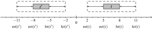
Scheduling propagators. An important application area is constraint-based scheduling, see for example [2]. Many propagation algorithms for constraint-based scheduling are based on tasks, where a task t is characterized by its start time, processing time (how long does the task take to be executed on a resource), and end time. Scheduling algorithms are typically expressed in terms of earliest start time (est ( t ) ), latest start time (lst ( t ) ), earliest completion time (ect ( t ) ), and latest completion time (lct ( t ) ).

Another particular aspect of scheduling algorithms is that they are often required in two, mutually dual, variants. Let us consider not-first/not-last propagation as an example. Assume a set of tasks T and a task t /negationslash∈ T to be scheduled on the same resource. Then t cannot be scheduled before the tasks in T ( t is not-first in T ∪{ t } ), if ect ( t ) > lst ( T ) (where lst ( T ) is a conservative estimate of the latest start time of all tasks in T ). Hence, est ( t ) can be adjusted to leave some room for at least one task from T . The dual variant is that t is not-last: if ect ( T ) > lst ( t ) (again, ect ( T ) estimates the earliest completion time of T ), then lct ( t ) can be adjusted.

Running the dual variant of a scheduling algorithm on tasks t ∈ T is the same as running the original algorithm on the dual tasks t ′ ∈ T ′ , which are simply mirrored at the 0-origin of the time scale (see Figure 1):

The dual variant of a scheduling propagator can be automatically derived using a minus view that transforms the time values. In our example, only a propagator for not-first

needs to be implemented and the propagator for not-last can be derived (or vice versa). This is in particular beneficial if the algorithms use sophisticated data structures such as Ω -trees [37]. Here, also the data structure needs to be implemented only once and the dual data structure for the dual propagator is derived.

4.2 Generalization

Common views for integer variables capture linear transformations of the integer values: an offset view for o ∈ Z on x is defined as ϕ x ( v ) = v + o , and a scale view for a ∈ Z on x is defined as ϕ x ( v ) = av .

Offset and scale views are useful for generalizing propagators. Generalization has two key advantages: simplicity and efficiency. A more specialized propagator is often simpler to implement (and simpler to implement correctly) than a generalized version. The specialized version can save memory and runtime during execution.

We can devise an efficient propagation algorithm for a linear equality constraint ∑ n i = 1 xi = c for the common case that the linear equation has only unit coefficients. The more general case ∑ n i = 1 aixi = c can be derived by using scale views for ai on xi (the same technique of course applies to linear inequalities and disequality rather than equality). Similarly, a propagator for all-different ( x 1 , . . . , xn ) can be generalized to all-different ( c 1 + x 1 , . . . , cn + xn ) by using offset views for ci ∈ Z on xi . Likewise, from a propagator for the element constraint a [ x ] = y for integers a 1 , . . . , an and integer variables x and y , we can derive the generalized version a [ x + o ] = y with an offset view, where o ∈ Z provides a useful offset for the index variable x .

These generalizations can be applied to domain- as well as bounds-complete propagators. While most Boolean propagators are domain-complete, bounds completeness plays an important role for integer propagators. Section 3.3 shows that, given appropriate hull-surjective and/or hull-injective views, the different notions of bounds consistency are preserved when deriving propagators.

The views for integer variables presented in this section have the following properties: minus and offset views are hull-bijective, whereas a scale view for a ∈ Z on x is always hull-injective and only hull-surjective if a = 1 or a = -1 (in which cases it coincides with the identity view or a minus view, respectively).

4.3 Specialization

We employ constant views to specialize propagators. A constant view behaves like an assigned variable. In practice, specialization has two advantages. Fewer variables require less memory. And specialized propagators can be compiled to more efficient code, if the constants are known at compile time.

Examples for specialization are

• ■ a propagator for binary linear inequality x + y ≤ c derived from a propagator for x + y + z ≤ c by using a constant 0 for z ;
• ■ a reified propagator for ( x = c ) ↔ b from ( x = y ) ↔ b and a constant c for y ;
• ■ propagators for the counting constraints | { i | xi = c }| = z and | { i | xi = y }| = c from a propagator for | { i | xi = y }| = z ;
• ■ a propagator for set disjointness from a propagator for x ∩ y = z and a constant empty set for z ; and many more.

Wehaveto straightforwardly extend the model for constant views. Propagators may now be defined with respect to a superset of the variables, X ′ ⊇ X . A constant view for the value k on a variable z ∈ X ′ \ X translates between the two sets of variables:

Here, a [ k / z ] means augmenting the assignment a so that it maps z to k , and a | X is the functional restriction of a to the set X .

It is important that this definition preserves failure. If a propagator returns a failed domain d that maps z to the empty set, then ϕ -( d ) is the empty set, too (recall that this is really ϕ -( con ( d )) , and con ( d ) = / 0 if d ( z ) = / 0).

4.4 Type Conversion

A type conversion view lets propagators for one type of variable work with a different type, by translating the underlying representation. Our model already accommodates for this, as a view ϕ x maps elements between different sets V and V ′ .

Integer views. Boolean variables are essentially integer variables restricted to the values { 0 , 1 } . Constraint programming systems may choose a more efficient implementation for Boolean variables and hence the variable types for integer and Boolean variables differ. By wrapping an efficient Boolean variable in an integer view , all integer propagators can be directly reused with Boolean variables. This can save substantial effort: for example, an implementation of the regular -constraint for Boolean variables can be derived which is actually useful in practice [19].

Singleton set views. A singleton set view on an integer variable x , defined as ϕ x ( v ) = { v } , presents an integer variable as a set variable. Many constraints involve both integer and set variables, and some of them can be expressed with singleton set views. A simple constraint is x ∈ y , where x is an integer variable and y a set variable. Singleton set views derive it as { x } ⊆ y . This extends to { x }/diamondmath y for all other set relations /diamondmath .

Singleton set views can also be used to derive pure integer constraints from set propagators. For example, the constraint same ( x 1 , . . . , xn , y 1 , . . . , ym ) with integer variables xi , yi states that the variables xi take the same values as the variables yi . With singleton set views, ⋃ n i = 1 { xi } = ⋃ m j = 1 { yj } implements this constraint (albeit with weaker propagation than the algorithm presented in [4]).

Set bounds and complete set domain variables. Most systems approximate set variable domains as set intervals defined by lower and upper bounds [25, 13]. However, [16] introduces a representation for the complete domains of set variables, using ROBDDs. Type conversion views can translate between set interval and ROBDDbased implementations. We can derive a propagator on ROBDD-based variables from a set interval propagator, and thus reuse set interval propagators for which no efficient ROBDD representation exists.

4.5 Applicability and Return on Investment

To get an overview of how applicable the presented techniques for propagator derivation are, let us consider the use of views in Gecode (version 3.1.0). Table 1 shows the number of propagator implementations and the number of propagators derived from the

Table 1: Number of implemented vs. derived propagators

Variable type	Implemented	Derived	Ratio
Integer	77	400	5 . 19
Boolean	28	91	3 . 25
Set	28	122	4 . 36
Overall	133	613	4 . 61

class IntVar { private : int _min, _max; public : int min( void ) { return _min; } int max( void ) { return _max; } void adjmin( int n) { if (n > _min) _min = n; } void adjmax( int n) { if (n < _max) _max = n; } }; class OffsetView { protected : IntVar* x; int o; public : OffsetView(IntVar* x0, int o0) : x(x0), o(o0) {} int min( void ) { return x->min()+o; } int max( void ) { return x->max()+o; } void adjmin( int n) { x->adjmin(n-o); } void adjmax( int n) { x->adjmax(n-o); } };

implementations. On average, every propagator implementation results in 4.6 derived propagators. Propagator implementations in Gecode account for more than 40000 lines of code and documentation. As a rough estimate, deriving propagators using views thus saves around 140000 lines of code and documentation to be written, tested, and maintained. On the other hand, the views mentioned in this section are implemented in less than 8000 lines of code, yielding a 1750% return on investment.

5 Implementation

This section presents an implementation architecture for views and derived propagators, based on making propagators parametric . Deriving a propagator then means instantiating a parametric propagator with views. The presented architecture is an orthogonal layer of abstraction on top of any solver implementation.

5.1 Views

The model introduced views as functions that transform the input and output of a propagator, which maps domains to domains. In an object-oriented implementation of this model, a propagator is no longer a function, but an object with a propagate method that accesses and modifies a domain through the methods of variable objects. Such an object-oriented model is used for example by ILOG Solver [27] and Choco [18], and is the basis of most of the current propagation-based constraint solvers.

Figure 2 shows C ++ classes for a simple integer variable (just representing bounds information) and a corresponding offset view. The view has the same interface as the variable, so that it can be used in its place. It contains a pointer to the underlying integer variable and delegates all the operations, performing the necessary transformations.

template < class VX, class VY> class Eq : public Propagator { protected : VX* x; VY* y; public : Eq(VX* x0, VY* y0) : x(x0), y(y0) {} virtual void propagate( void ) { x->adjmin(y->min()); x->adjmax(y->max()); y->adjmin(x->min()); y->adjmax(x->max()); } };

5.2 Deriving Propagators

In order to derive a propagator using view objects like the above, we use parametricity , a mechanism provided by the implementation language that supports the instantiation of the same code (the propagator) with different parameters (the views).

Figure 3 shows a simple equality propagator. The propagator is based on C ++ templates, it is parametric over the types of the two views it uses and can be instantiated with any view that provides the necessary operations. This type of parametricity is called parametric polymorphism , and is available in other programming languages for example in the form of Java generics [14] or Standard ML functors [22].

Given two pointers to integer variables x and y , the propagator can be instantiated to implement /llbracket x = y /rrbracket as follows (using the IntVar class from Figure 2):

new Eq

Events. Most constraint solvers schedule the execution of propagators according to events (see for example [31]). For example, a propagator p for /llbracket x < y /rrbracket can only prune the domain (and thus should only be executed) if either the lower bound of x or the upper bound of y changes, written lbc ( x ) and ubc ( y ) . We say that p subscribes to the event set { lbc ( x ) , ubc ( y ) } .

Now assume that p ′ is derived from p using minus views on x and y , thus implementing x > y . Obviously, p ′ should subscribe to the dual event set, { ubc ( x ) , lbc ( y ) } . In the implementation, views provide all the operations needed for event handling (such as subscription) and perform the necessary transformations of event sets.

5.3 Parametricity

Independent of the concrete implementation, views form an orthogonal layer of abstraction on top of any propagation-based constraint solver. As long as the implementation language provides some kind of parametricity, and variable domains are accessed through some form of variable objects, propagators can be derived using views.

In addition to parametric polymorphism, two other forms of parametricity exist, functional parametricity and dynamic binding . Functional parametricity means that in languages such as Standard ML [22] or Haskell [24], a higher-order function is parametric over its arguments. Dynamic binding is typically coupled with inheritance in object-oriented languages (virtual function calls in C ++ , method calls in Java). Even

in languages that lack direct support for parametricity, parametric behavior can often be achieved using other mechanisms, such as macros or function pointers in C.

Choice of parametricity. In C ++ , parametric polymorphism and dynamic binding have advantages and disadvantages as it comes to deriving propagators.

Templates are compiled by monomorphization: the code is replicated and specialized for each instance. The compiler can generate optimized code for each instance, for example by inlining the transformations that a view implements.

Achieving high efficiency in C ++ with templates sacrifices some expressiveness. Instantiation can only happen at compile-time. Hence, either C ++ must be used for modeling, or all potentially required propagator variants must be instantiated explicitly. The choice which propagator to use can however be made at runtime: for linear equations, for instance, if all coefficients are units, the optimized original propagator can be posted.

For n -ary constraints, compile-time instantiation can be a limitation, as all arrays must be monomorphic (contain only a single kind of view). For example, one cannot mix scale and minus views in linear constraints. For some propagators, we can work around this restriction using more than a single array of views. For example, a propagator for a linear constraint can employ two arrays of different view types, one of which may then be instantiated with identity views and the other with minus views. While this poses a limitation in principle, our experience from Gecode suggests that there are only few propagators in practice that suffer from this limitation.

Dynamic binding is more flexible than parametric polymorphism, as instantiation happens at runtime and arrays can be polymorphic. This flexibility comes at the cost of reduced efficiency, as the transformations done by view operations typically cannot be inlined and optimized, but require additional virtual method calls. Section 7 evaluates empirically how these virtual method calls affect performance.

Compile-time versus runtime constants. Some views involve a parameter, such as the coefficient of a scale view or the constant of a constant view. These parameters can again be instantiated at compile-time or at runtime. For instance, one can regard a minus view as a compile-time specialization of a scale view with coefficient -1, and a zero view may specialize a constant view. With the constants being known at compile-time, the compiler can apply more aggressive optimizations.

5.4 Iterators

Typical domain operations involve a single integer value, for instance adjusting the minimum or maximum of an integer variable. These operations are not efficient if a propagator performs full domain reasoning on integer variables or deals with set variables. Therefore, set-valued operations, like updating a whole integer variable domain to a new set, or excluding a set of elements from a set variable domain, are important for efficiency. Many constraint programming systems provide an abstract set-datatype for accessing and updating variable domains, as for example in Choco [6], ECL i PS e [8], SICStus Prolog [35], and Mozart [23]. ILOG Solver [17] only allows access by iterating over the values of a variable domain.

This section develops iterators as one particular abstract datatype for set-valued operations on variables and views. There are two main reasons to discuss iterators in this paper. First, iterators provide simple, expressive, and efficient set-valued operations on

variables. Second, and more importantly, iterators transparently perform the transformations needed for set-valued operations on views, and thus constitute a perfect fit for deriving propagators.

Range sequences and range iterators. A range [ m .. n ] denotes the set of integers { l ∈ Z | m ≤ l ≤ n } . A range sequence ranges ( S ) for a finite set of integers S ⊆ Z is the shortest sequence s = 〈 [ m 1 .. n 1 ] , . . . , [ mk .. nk ] 〉 such that S = ⋃ k i = 1 [ mi .. ni ] and the ranges are ordered by their smallest elements ( mi ≤ mi + 1 for 1 ≤ i < k ). We thus define the set covered by a range sequence as set ( s ) = ⋃ k i = 1 [ mi .. ni ] . The above range sequence is also written as 〈 [ mi .. ni ] 〉 k i = 1 . Clearly, the range sequence of a set is unique, none of its ranges is empty, and ni + 1 < mi + 1 for 1 ≤ i < k .

A range iterator for a range sequence s = 〈 [ ni .. mi ] 〉 k i = 1 is an object that provides iteration over s : each of the [ mi .. ni ] can be obtained in sequential order but only one at a time. A range iterator r provides the following operations: r . done () tests whether all ranges have been iterated, r . next () moves to the next range, and r . min () and r . max () return the minimum and maximum value for the current range. By set ( r ) we refer to the set defined by an iterator r (which must coincide with set ( s ) ).

A range iterator naturally hides its implementation. It can iterate a sequence (for instance an array) directly by position, but it can just as well traverse a linked list or the leaves of a balanced tree, or for example iterate over the union of two other iterators.

Iterators are consumed by iteration. Hence, if the same sequence needs to be iterated twice, a fresh iterator is needed. If iteration is cheap, an iterator can support multiple iterations by providing a reset operation. Otherwise, a cache iterator takes an arbitrary range iterator as input, iterates it completely, and stores the obtained ranges in an array. Its operations then use the array. The cache iterator implements a reset operation, so that the possibly costly input iterator is used only once, while the cache iterator can be used as often as needed.

Iterators for variables. The two basic set-valued operations on integer variables are domain access and domain update. For an integer variable x , the operation x . getdom () returns a range iterator for ranges ( d ( x )) . The operation x . setdom ( r ) updates the variable domain of x to set ( r ) given a range iterator r , provided that set ( r ) ⊆ d ( x ) . The responsibility for ensuring that set ( r ) ⊆ d ( x ) is left to the programmer.

In order to provide safer and richer operations, we can use iterator combinators . For example, an intersection iterator r = iinter ( r 1 , r 2 ) combines two range iterators r 1 and r 2 such that set ( r ) = set ( r 1 ) ∩ set ( r 2 ) . Similarly, a difference iterator r = iminus ( r 1 , r 2 ) yields set ( r ) = set ( r 1 ) \ set ( r 2 ) .

Richer set-valued operations are then effortless. The operation x . adjdom ( r ) adjusts the domain d ( x ) by set ( r ) , yielding d ( x ) ∩ set ( r ) , whereas x . excdom ( r ) excludes set ( r ) from d ( x ) , yielding d ( x ) \ set ( r ) :

x . adjdom ( r ) = x . setdom ( iinter ( x . getdom () , r )) x . excdom ( r ) = x . setdom ( iminus ( x . getdom () , r ))

In contrast to the x . setdom ( · ) operation, the richer set-valued operations are inherently contracting, and thus safer to use when implementing a propagator.

Iterators also serve as the natural interface for operations on set variables, which are usually approximated as set intervals defined by a lower and an upper bound [25, 13]:

d ( x ) = [ glb ( d ( x )) .. lub ( d ( x ))] = { s | glb ( d ( x )) ⊆ s , s ⊆ lub ( d ( x )) }

In order to access and update these set bounds, propagators use set-valued operations based on iterators: x . glb () returns a range iterator for ranges ( glb ( d ( x ))) , x . lub () returns a range iterator for ranges ( lub ( d ( x ))) , x . adjglb ( r ) updates the domain of x to [ glb ( d ( x )) ∪ set ( r ) , lub ( d ( x ))] , and x . adjlub ( r ) updates the domain of x to [ glb ( d ( x )) , lub ( d ( x )) ∩ set ( r )] .

Iterator combinators provide the operations that set propagators need: union, intersection, difference, and complement. Many propagators can thus be implemented directly using iterators and do not require any temporary data structures for storing set-valued intermediate results.

All set-valued operations are parametric with respect to the iterator r : any range iterator can be used. As for parametric propagators, an implementor has to decide on the kind of parametricity to use. Gecode uses template-based parametric polymorphism, with the performance benefits due to monomorphization and consequent code optimization mentioned previously.

Advantages. Range iterators provide essential advantages over an explicit set representation. First, any range iterator regardless of its implementation can be used in domain operations. This turns out to result in simple, efficient, and expressive domain updates. Second, no costly memory management is required to maintain a range iterator as it provides access to only one range at a time. Third, the abstractness of range iterators makes them compatible with views and derived propagators: the necessary view transformations can be encapsulated in an iterator, as discussed below.

Iterators for views. As iterators hide their implementation, they are perfectly suited for implementing the transformations required for set-valued operations on views.

Set-valued operations for constant integer views are straightforward. For a constant view v on constant k , the operation v . getdom () returns an iterator for the singleton range sequence 〈 [ k .. k ] 〉 . The operation v . setdom ( r ) just checks whether the range sequence of r is empty (in order to detect failure).

Set-valued operations for an offset view are provided by an offset iterator . For a range sequence r = 〈 [ mi .. ni ] 〉 k i = 1 and offset c , ioffset ( r , c ) iterates 〈 [ mi + c .. ni + c ] 〉 k i = 1 . An offset view on x with offset c then implements getdom as ioffset ( x . getdom () , c ) and setdom ( r ) as x . setdom ( ioffset ( r , -c )) .

For minus views we just give the range sequence, iteration is obvious. For a given range sequence 〈 [ mi .. ni ] 〉 k i = 1 , the negative sequence is obtained by reversal and sign change as 〈 [ -nk -i + 1 .. -mk -i + 1 ] 〉 k i = 1 . The same iterator for this sequence can be used both for setdom and getdom operations. Note that implementing the iterator is involved as it changes direction of the range sequence. There are two different options for changing direction: either the set-valued operations accept iterators in both directions or a cache iterator is used to reverse the direction. Gecode uses the latter and Section 7.2 evaluates the overhead introduced by cache iterators.

A scale iterator provides the necessary transformations for scale views. Assume a scale view on a variable x with a coefficient a > 0, and let 〈 [ mi .. ni ] 〉 k i = 1 be a range sequence for d ( x ) . If a = 1, the scale iterator does not change the range sequence. Otherwise, the corresponding scaled range sequence is 〈{ a × m 1 } , { a × ( m 1 + 1 ) } , . . . , { a × n 1 } , . . . , { a × mk } , { a × ( mk + 1 ) } , . . . , { a × nk }〉 . For the other direction, assume we want to update the domain using a set S through a scale view. Assume that 〈 [ mi .. ni ] 〉 k i = 1 is a range sequence for S . Then for 1 ≤ i ≤ k the ranges [ /ceilingleft mi / a /ceilingright .. /floorleft ni / a /floorright ] correspond to the required variable domain for x , however they do not necessarily form a range

sequence as the ranges might be empty, overlapping, or adjacent. Iterating the range sequence is however simple by skipping empty ranges and merging overlapping or adjacent ranges. Scale views for a variable x and a coefficient a in Gecode are restricted to be strictly positive so as to not change the direction of the scaled range sequence. A negative coefficient can be obtained by using a scale view together with a minus view.

A complement view of a set variable x uses a complement iterator , which given a range iterator r iterates over set ( r ) .

6 Limitations

Although views are widely applicable, they are no silver bullet. This section explores some limitations of the presented model.

Beyond injective views. Views are required to be injective, as otherwise ϕ - ◦ ϕ is no longer the identity function, and derived propagators would not necessarily be contracting. An example for this behavior is a view for the absolute value of an integer variable. Assuming a variable domain d ( x ) = { 1 } , an absolute value view ϕ would leave the domain as it is, ϕ ( d )( x ) = { 1 } , but the inverse would 'invent' the negative value, ϕ -( ϕ ( d ))( x ) = {-1 , 1 } . With an adapted definition of derived propagators, such as ̂ ϕ ( p )( d ) = ϕ -( p ( ϕ ( d ))) ∩ d , non-injective views could be used - however, many of the proofs in this paper rely on injectivity (though some of the theorems possibly still hold for non-injective views).

Multi-variable views. Some multi-variable views that seem interesting for practical applications do not preserve contraction, for instance a view on the sum or product of two variables. The reason is that removing a value through the view would have to result in removing a tuple of values from the domain. As domains can only represent Cartesian products, this is not possible in general. Such a view would have two main disadvantages. First, if propagation of the original constraint is strong but does not lead to an actual domain pruning through the views, then the potentially high computational cost for the pruning does not pay off. A cheaper but weaker, dedicated propagation algorithm or a different modeling with stronger pruning is then a better choice. Second, if views do not preserve contraction, then Proposition 5 does not hold. That means that a propagator p cannot easily detect subsumption any longer, as it would have to detect it for ̂ ϕ ( p ) instead of just for itself, p . Systems such as Gecode that disable subsumed propagators (as described in [33]) then lose this potential for optimization.

For contraction-preserving views on multiple variables, all the theorems still hold. Two such views we could identify are a set view of Boolean variables [ b 1 , . . . , bn ] , behaving like { i | bi = 1 } ; and an integer view of Boolean variables [ b 1 , . . . , bn ] , where bi is 1 if and only if the integer has value i ; as well as the inverse views of these two.

Propagator invariants. Propagators typically rely on certain invariants of a variable domain implementation. If idempotency or completeness of a propagator depend on these invariants, type conversion views lead to problems, as the actual variable implementation behind the view may not respect the same invariants.

For example, a propagator for set variables based on the set interval approximation can assume that adjusting the lower bound of a variable does not affect its upper bound. If this propagator is instantiated with a type conversion view for an ROBDD-based set

Table 2: Results for Gecode 3.1.0, the baseline for the experiments

Benchmark	time (ms)	mem. (KByte)	failures	propagations
All-Interval (50)	183 . 21	148	0	6685
All-Interval (100)	3904 . 21	516	0	25866
Alpha (naive)	100 . 00	23	7435	136179
BIBD (7-3-60)	1762 . 85	4516	1306	921686
Eq-20	1 . 52	14	54	3460
Golomb Rulers (Bnd, 10)	423 . 39	67	8890	1181704
Golomb Rulers (Dom, 10)	607 . 86	419	8890	1181770
Graph Coloring	324 . 46	3910	1100	125264
Magic Sequence (Smart, 500)	251 . 50	4484	251	84302
Magic Sequence (GCC, 500)	305 . 15	330	251	3908
Partition (32)	5928 . 04	265	160258	12107504
Perfect Square	185 . 54	3972	150	305391
Queens (10)	36 . 88	27	4992	43448
Queens (Dom, 10)	103 . 38	99	3940	59508
Queens (100)	1 . 54	235	22	455
Queens (Dom, 100)	31 . 83	2056	8	693
Sorting (400)	1400 . 01	151413	0	459501
Social Golfers (8-4-9)	193 . 37	10254	32	181290
Social Golfers (5-3-7)	1199 . 51	2117	1174	852391
Hamming Codes (20-3-32)	1140 . 98	24746	2296	753751
Steiner Triples (9)	120 . 11	901	1067	297501
Sudoku (Set, 1)	3 . 48	83	0	1820
Sudoku (Set, 4)	7 . 30	148	1	3752
Sudoku (Set, 5)	55 . 14	514	25	28038

variable (see Section 4.4), this invariant is violated: if, for instance, the current domain is {{ 1 , 2 } , { 3 }} , and 1 is added to the lower bound, then 3 is removed from the upper bound (in addition to 2 being added to the lower bound). If a propagator reports that it has computed a fixed point based on the assumption that the upper bound cannot have changed, it may actually not be at a fixed point. This potentially results in incorrect propagation, for instance if the propagator could detect failure if it were run again.

7 Evaluation

While Section 3 proved that derived propagators are perfect with respect to the mathematical model, this section shows that in most cases one can also obtain perfect implementations of derived propagators, not incurring any performance penalties compared to dedicated, handwritten propagators.

Experimental setup. The experiments are based on Gecode 3.1.0, compiled using the GNU C ++ compiler gcc 4.3.2, on an Intel Pentium IV at 2.8 GHz running Linux. Runtimes are the average of 25 runs, with a coefficient of deviation less than 2.5% for all benchmarks. All example programs are available in the Gecode distribution. Table 2 shows the figures for the unmodified Gecode 3.1.0 (pure integer models above, models with integer and set variables below the horizontal line), and results will be given relative to these numbers. For example, a runtime of 130% means that the example needs 30% more time, while 50% means that it is twice as fast as in Gecode 3.1.0. The column time shows the runtime, mem. the peak allocated memory, failures the number of failures during search, and propagations the number of propagator invocations.

Table 3: Relative performance of decomposition, compared to views

Benchmark	time%	mem. %	propagations %
Alpha (naive)	412 . 88	360 . 87	673 . 83
BIBD (7-3-60)	308 . 80	211 . 94	256 . 12
Eq-20	590 . 35	700 . 00	704 . 57
Partition (32)	135 . 61	113 . 58	136 . 40
Perfect Square	114 . 46	109 . 67	104 . 42
Queens (Dom, 10)	173 . 32	100 . 00	519 . 68
Queens (Dom, 100)	140 . 60	103 . 11	2371 . 86
Social Golfers (8-4-9)	335 . 89	234 . 82	160 . 22
Social Golfers (5-3-7)	217 . 28	190 . 69	150 . 58
Hamming Codes (20-3-32)	113 . 81	104 . 66	99 . 65
Steiner Triples (9)	132 . 79	100 . 00	101 . 76
Sudoku (Set, 1)	166 . 18	100 . 00	110 . 38
Sudoku (Set, 4)	152 . 82	110 . 81	107 . 06
Sudoku (Set, 5)	143 . 63	100 . 00	105 . 47

As many of the experimental results rely on the optimization capabilities of the used C ++ compiler, we verified that all experiments yield similar results with the Microsoft Visual Studio 2008 C ++ compiler.

7.1 Views Versus Decomposition

In order to evaluate whether deriving propagators is worth the effort in the first place, this set of experiments compares derived propagators with their decompositions, revealing a significant overhead of the latter.

Table 3 shows the results of these experiments. For Alpha and Eq-20 , linear equations with coefficients are decomposed. For Queens 100 , we replace the special alldifferent -with-offsets by its decomposition into an all-different propagator and binary equality-with-offset propagators. In BIBD and Perfect Square , we decompose ternary Boolean propagators, implementing x ∧ y ↔ z as ¬ x ∨¬ y ↔¬ z in BIBD , and x ∨ y ↔ z as ¬ x ∧¬ y ↔¬ z in Perfect Square . In the remaining examples, we decompose a set intersection into complement and union propagators.

Some integer examples show a significant overhead of around six times the runtime and memory when decomposed. The overhead of most set examples as well as Perfect Square is moderate, partly because no additional variable was introduced if the model already contained its complement or negation. As to be expected, decomposition often needs significantly more propagation steps, but as the additional steps are performed by cheap propagators (like x = y + i or x = ¬ y ), the runtime effect is less drastic. Queens 100 is an extreme case, where 23 times the propagation steps only cause 40% more runtime. The reason is that the scheduling order does not take advantage of the fact that the decompositions are Berge-acyclic as discussed in Section 3.5. Partition 32 has a single linear equation with coefficients, several linear equations with unit coefficients, multiplications, and a single all-different . Replacing the linear equation by its decomposition has little effect on the runtime (35% overhead).

7.2 Impact of Derivation Techniques

The techniques presented in Section 4 have different impacts on the performance of the derived propagators.

Table 4: Relative performance of minus views

Benchmark	time%	prop. %	Benchmark	time%	prop. %
All-Interval (50)	100 . 00	100 . 00	Partition (32)	131 . 83	135 . 95
All-Interval (100)	100 . 52	100 . 00	Queens (10)	98 . 32	100 . 00
Alpha (naive)	101 . 81	100 . 00	Queens (Dom, 10)	107 . 63	100 . 00
Golomb Rulers (Bnd, 10)	99 . 36	100 . 01	Queens (100)	97 . 83	100 . 00
Golomb Rulers (Dom, 10)	107 . 77	100 . 18	Queens (Dom, 100)	95 . 62	100 . 00
Graph Coloring	107 . 19	99 . 84	Sorting (400)	105 . 13	100 . 00

Generalization and specialization. These techniques can be implemented without any performance overhead compared to a handwritten propagator. This is not surprising as the only potential overhead could be that a function call is not resolved at compile time. For example, a thorough inspection of the code generated by the GNU C ++ compiler and the Microsoft Visual Studio C ++ compiler shows that they are able to fully inline the operations of offset and scale views.

Transformation and type conversion. These techniques can incur an overhead compared to a dedicated implementation, as the transformations performed by the views can sometimes not be removed by compiler optimizations, and type conversions may be costly if the data structures for the variable domains differ significantly.

For example, a propagator instantiated with two minus views of variables x and y may include a comparison, ( -x ) < ( -y ) . Due to the invariants guaranteed by views, this is equivalent to y < x , saving two negations. However, the asymmetry in the two's complement representation of integers prevents the compiler from performing this optimization. As an experiment to evaluate this effect, we instantiated an all-different propagator with minus views. The resulting derived propagator of course implements the same constraint, but incurs the overhead of negation. Similarly, we replaced the max propagator in the Sort example with a min (where the propagator for min is derived from the propagator for max) and negated all parameters. According to the results in Table 4, the overhead is often negligible, and only exceeds 5% in examples that use the domain-complete all-different propagator ( Graph Coloring , Golomb Rulers Dom and Queens Dom ) or predominantly min propagators ( Sort ). Queens Dom 100 does not show the effect as the runtime is dominated by search. Using minus views can result in different propagator scheduling. The Partition example shows this behavior, where the increase in propagation steps results in increased runtime.

It is interesting to note that the domain-complete all-different propagator, when instantiated with minus views, requires a cache iterator for sequence reversal (as discussed in Section 5.4). Surprisingly, the overhead of minus views is largely independent of the use of cache iterators which is confirmed in Section 7.4.

Other transformations are translated optimally, such as turning ( -x ) -( -y ) into y -x . Boolean negation views also lead to optimal code, as they do not compute 1 -x for a Boolean variable x , but instead swap the positive and negative operations.

Set-valued transformations can result in non-optimal code. For example, a propagator for ternary intersection, x = y ∩ z , will include an inference x . adjglb ( y . glb () ∩ z . glb ()) . To derive a propagator for x = y ∪ z , we instantiate the intersection propagator with complement views for x , y , and z , yielding the following inference:

Table 5: Relative performance of views compared to dedicated set propagators

Benchmark	time%	Benchmark	time%
Social Golfers (8-4-9)	166 . 31	Sudoku (Set, 1)	167 . 44
Social Golfers (5-3-7)	148 . 83	Sudoku (Set, 4)	151 . 74
Hamming Codes (20-3-32)	129 . 11	Sudoku (Set, 5)	142 . 83
Steiner Triples (9)	127 . 85

Table 6: Relative performance of virtual method calls

Benchmark	time%	Benchmark	time%
All-Interval (50) All-Interval (100) Alpha (naive) BIBD (7-3-60) Eq-20 Golomb Rulers (Bnd, 10) Golomb Rulers (Dom, 10) Graph Coloring Magic Sequence (Smart, 500) Magic Sequence (GCC, 500) Partition (32) Perfect Square Queens (10) Queens (100)	182 . 63 113 . 20 153 . 59 138 . 50 211 . 69 220 . 01 170 . 13 104 . 29 136 . 58 226 . 64 187 . 89 130 . 64 133 . 81 160 . 79	Social Golfers (8-4-9) Social Golfers (5-3-7) Hamming Codes (20-3-32) Steiner Triples (9) Sudoku (Set, 1) Sudoku (Set, 4) Sudoku (Set, 5)	148 . 37 138 . 95 131 . 37 149 . 08 119 . 56 118 . 78 119 . 17

which amounts to computing

It would be more efficient to implement the equivalent x . adjlub ( y . lub () ∪ z . lub ()) because this requires three set operations less. Unfortunately, no compiler will find this equivalence automatically, as it requires knowledge about the semantics of the set operations. Table 5 compares a dedicated propagator for the constraint x ∩ y = z with a version using complement views and a propagator for x ∪ y = z . The overhead of 27% to 67% does not render views useless for set variables, but it is nevertheless significant.

7.3 Templates Versus Virtual Methods

As suggested in Section 5, in C ++ , compile-time polymorphism using templates is far more efficient than virtual method calls. To evaluate this, we changed the basic operations of integer variables to be virtual methods, such that view operations need one virtual method call. In addition, all operations that use templates (and can therefore not be made virtual in C ++ ) have been changed so that they cannot be inlined, to simulate virtual method calls. This is a conservative approximation of the actual cost of fully virtual views. The results of these experiments appear in Table 6. Virtual method calls cause a runtime overhead between 4% and 127% for the integer examples (left table), and 18% to 49% for the set examples (right table). The runtime overhead for set examples is lower as the basic operations on set variables are considerably more expensive than the basic operations on integer variables.

Table 7: Relative performance of cache iterators

Benchmark	time%	Benchmark	time%
All-Interval (50)	102 . 48	Social Golfers (8-4-9)	522 . 62
All-Interval (100)	101 . 17	Social Golfers (5-3-7)	450 . 15
Golomb Rulers (Bnd, 10)	100 . 51	Hamming Codes (20-3-32)	297 . 38
Golomb Rulers (Dom, 10)	128 . 98	Steiner Triples (9)	304 . 97
Graph Coloring	144 . 58	Sudoku (Set, 1)	459 . 85
Magic Sequence (GCC, 500)	103 . 56	Sudoku (Set, 4)	483 . 27
Queens (Dom, 10)	187 . 36	Sudoku (Set, 5)	436 . 92
Queens (Dom, 100)	155 . 62

7.4 Iterators Versus Temporary Data Structures

The following experiments show that using range iterators improves the efficiency of propagators, compared to the use of explicit set data structures for temporary results.

For the experiments, temporary data structures have been emulated by wrapping all iterators in a cache iterator as described in Section 5.4. Table 7 shows the results. For integer propagators that perform the safe iterator-based domain operations introduced in Section 5.4, computing with temporary data structures results in 28% to 87% overhead ( Golomb Rulers Dom, Graph Coloring, Queens Dom ). For set propagators, which make much more use of iterators than integer propagators, the overhead becomes prohibitive, resulting in up to 4.8 times the runtime. The memory consumption does not increase, because iterators are not stored, and only few iterators are active at a time.

8 Conclusion

The paper has developed views for deriving propagator variants. Such variants are ubiquitous, and the paper has shown how to systematically derive propagators using different types of views, corresponding to techniques such as transformation, generalization, specialization, and type conversion.

Based on a formal, implementation independent model of propagators and views, the paper has identified fundamental properties of views that result in perfect derived propagators. The paper has shown that a derived propagator inherits correctness and domain completeness from its original propagator, and bounds completeness given additional properties of the used views.

The paper has presented an implementation architecture for views based on parametricity . The propagator implementation is kept parametric over the type of view that is used, so that deriving a propagator amounts to instantiating a parametric propagator with the proper views. This implementation architecture is an orthogonal layer of abstraction that can be implemented on top of any constraint solver.

An empirical evaluation has shown that views have proven invaluable for the implementation of Gecode, saving huge amounts of code to be written and maintained. Furthermore, deriving propagators using templates in C ++ has been shown to yield competitive (in most cases optimal) performance compared to dedicated handwritten propagators. The experiments have also clarified that deriving propagators is vastly superior to decomposing the constraints into additional variables and simple propagators.

Acknowledgments. We thank Mikael Lagerkvist, Gert Smolka, and Thibaut Feydy for fruitful discussions. Christian Schulte has been partially funded by the Swedish

Research Council (VR) under grant 621-2004-4953.

References

1. Krzysztof R. Apt. Principles of Constraint Programming . Cambridge University Press, Cambridge, UK, 2003.
2. Philippe Baptiste, Claude Le Pape, and Wim Nuijten. Constraint-based Scheduling . International Series in Operations Research & Management Science. Kluwer Academic Publishers, 2001.
3. Catriel Beeri, Ronald Fagin, David Maier, and Mihalis Yannakakis. On the desirability of acyclic database schemes. Journal of the ACM , 30(3):479-513, 1983.
4. Nicolas Beldiceanu, Irit Katriel, and Sven Thiel. Filtering algorithms for the same constraint. In R´ egin and Rueher [29], pages 65-79.
5. Mats Carlsson, Greger Ottosson, and Bj¨ orn Carlson. An o pen-ended finite domain constraint solver. In Hugh Glaser, Pieter H. Hartel, and Herbert Kuchen, editors, Programming Languages: Implementations, Logics, and Programs , volume 1292 of LNCS , pages 191-206, Southampton, UK, September 1997. Springer.
6. CHOCO. choco-solver.net , 2009.
7. Chiu Wo Choi, Warwick Harvey, Jimmy Ho-Man Lee, and Peter J. Stuckey. Finite domain bounds consistency revisited. In Abdul Sattar and Byeong-Ho Kang, editors, AI 2006: Advances in Artificial Intelligence , volume 4304 of LNCS , pages 49-58. Springer, 2006.
8. ECL i PS e . www.eclipse-clp.org , 2009.
9. Niklas E´ en and Niklas S¨ orensson. An extensible SAT-solver. In Enrico Giunchiglia and Armando Tacchella, editors, Theory and Applications of Satisfiability Testing , volume 2919 of LNCS , pages 502-518, Santa Margherita Ligure, Italy, May 2004. Springer.
10. Gecode. www.gecode.org , 2009.
11. Ian P. Gent, editor. Fifteenth International Conference on Principles and Practice of Constraint Programming , volume 5732 of LNCS , Lisbon, Portugal, September 2009. Springer. To appear.
12. Ian P. Gent, Christopher Jefferson, and Ian Miguel. Watched literals for constraint propagation in Minion. In Fr´ ed´ eric Benhamou, editor, Twelfth Internation Conference on Principles and Practice of Constraint Programming , volume 4204 of LNCS , pages 182-197, Nantes, France, September 2006. Springer.
13. Carmen Gervet. Conjunto: Constraint logic programming with finite set domains. In Maurice Bruynooghe, editor, International Symposium on Logic Programming , pages 339-358, Ithaca, NY, USA, 1994. MIT Press.
14. James Gosling, Bill Joy, Guy Steele, and Gilad Bracha. The Java Language Specification . Addison-Wesley Professional, third edition, 2005.

1. Warwick Harvey and Peter J. Stuckey. Improving linear constraint propagation by changing constraint representation. Constraints , 7:173-207, 2003.
2. Peter Hawkins, Vitaly Lagoon, and Peter J. Stuckey. Solving set constraint satisfaction problems using ROBDDs. Journal of Artificial Intelligence Research , 24:109-156, 2005.
3. ILOG Solver, part of ILOG CP. www.ilog.com/products/cp , 2009.
4. Franc ¸ois Laburthe. Choco: Implementing a CP kernel. In Nicolas Beldiceanu, Warwick Harvey, Martin Henz, Franc ¸ois Laburthe, Eric Monfroy, Tobias M¨ uller, Laurent Perron, and Christian Schulte, editors, Proceedings of TRICS: Techniques foR Implementing Constraint programming Systems, a post-conference workshop of CP 2000 , pages 71-85, September 2000.
5. Mikael Z. Lagerkvist and Gilles Pesant. Modeling irregular shape placement problems with regular constraints. In First Workshop on Bin Packing and Placement Constraints BPPC'08 , 2008.
6. Mikael Z. Lagerkvist and Christian Schulte. Propagator groups. In Gent [11]. To appear.
7. Alan Mackworth. Consistency in networks of relations. Artificial Intelligence , 8(1):99-118, 1977.
8. Robin Milner, Mads Tofte, and David MacQueen. The Definition of Standard ML . MIT Press, Cambridge, MA, USA, 1997.
9. The Mozart programming system. www.mozart-oz.org , 2009.
10. Simon L. Peyton Jones. Haskell 98. Journal of Functional Programming , 13(1), 2003.
11. Jean-Fran ¸ cois Puget. PECOS: A high level constraint programming language. In Proceedings of the first Singapore international conference on Intelligent Systems (SPICIS) , pages 137-142, Singapore, 1992.
12. Jean-Franc ¸ois Puget. A fast algorithm for the bound consistency of alldiff constraints. In Proceedings of the 15th National Conference on Artificial Intelligence , pages 359-366, Madison, WI, USA, July 1998. AAAI Press.
13. Jean-Franc ¸ois Puget. A C ++ implementation of CLP. In Proceedings of the Second Singapore International Conference on Intelligent Systems (SPICIS) , pages B256-B261, Singapore, November 1994.
14. Claude-Guy Quimper. Efficient Propagators for Global Constraints . PhD thesis, University of Waterloo, Canada, 2006.
15. Jean-Charles R´ egin and Michel Rueher, editors. Integration of AI and OR Techniques in Constraint Programming for Combinatorial Optimization Problems , volume 3011 of LNCS , Nice, France, April 2004. Springer.
16. Jean-Charles R ˜ A c © gin. A filtering algorithm for constraints of difference in CSPs. In Proceedings of the Twelfth National Conference on Artificial Intelligence , pages 362-367, Seattle, WA, USA, 1994. AAAI Press.

1. Christian Schulte and Mats Carlsson. Finite domain constraint programming systems. In Francesca Rossi, Peter van Beek, and Toby Walsh, editors, Handbook of Constraint Programming , Foundations of Artificial Intelligence, chapter 14, pages 495-526. Elsevier Science Publishers, Amsterdam, The Netherlands, 2006.
2. Christian Schulte and Peter J. Stuckey. When do bounds and domain propagation lead to the same search space? Transactions on Programming Languages and Systems , 27(3):388-425, May 2005.
3. Christian Schulte and Peter J. Stuckey. Efficient constraint propagation engines. Transactions on Programming Languages and Systems , 31(1):2:1-2:43, December 2008.
4. Christian Schulte and Guido Tack. Weakly monotonic propagators. In Gent [11]. To appear.
5. SICStus Prolog, 2009. www.sics.se/sicstus/ .
6. Pascal Van Hentenryck, Vijay A. Saraswat, and Yves Deville. Design, implementation, and evaluation of the constraint language cc(FD). Journal of Logic Programming , 37(1-3):293-316, 1998.
7. Petr Vil´ ım. O ( n log n ) filtering algorithms for unary resource constraint. In R´ egin and Rueher [29], pages 335-347.