Contents
2512.13190v1
WAY: Estimation of Vessel Destination in Worldwide AIS Trajectory
JIN SOB KIM HYUN JOON PARK WOOSEOK SHIN
Korea University, Seoul 02841, Republic of Korea
DONGIL PARK
SeaVantage, Seoul 06119, Republic of Korea
SUNG WON HAN
Korea University, Seoul 02841, Republic of Korea
AbstractThe Automatic Identification System (AIS) has recorded near-real-time vessel monitoring data over the years, paving the way for data-driven maritime surveillance methods; concurrently, the data suffer from unrefined, reliability issues and irregular intervals. In this paper, we address the problem of vessel destination estimation by exploiting the global-scope AIS data. We propose a differentiated data-driven approach recasting a long sequence of port-to-port international vessel trajectories as a nested sequence structure. Based on spatial grids, this approach mitigates the spatio-temporal bias of AIS data while preserving the detailed resolution of the original. Further, we propose a novel deep learning architecture (WAY) that is designed to effectively process the reformulated trajectory and perform the long-term estimation of the vessel destination ahead of arrival with a horizon of days to weeks. WAY comprises a trajectory representation layer and channel-aggregative sequential processing (CASP) blocks. The representation layer produces the multi-channel vector sequence output based on each kinematic and non-kinematic feature collected from AIS data. Then CASP blocks include multi-headed channeland self-attention architectures, where each processes aggregation and sequential information delivery respectively. Then, a taskspecialized learning technique, Gradient Dropout (GD), is also suggested for adopting many-to-many training along the trajectory progression on single labels. The technique prevents a surge of biased feedback by blocking the gradient flow stochastically using the condition depending on the length of training samples. Experimental results on 5-year accumulated AIS data demonstrated the superiority of WAY with recasting AIS trajectory compared to conventional spatial grid-based approaches, regardless of the trajectory progression steps. Moreover, the data proved that adopting GD
This research was supported by Brain Korea 21 FOUR. This research was also supported by Korea Institute for Advancement of Technology(KIAT) grant funded by the Korea Government(MOTIE) (P0008691, The Competency Development Program for Industry Specialist). (Corresponding author: Sung Won Han) .
Jin Sob Kim, Hyun Joon Park, Wooseok Shin, and Sung Won Han are with the School of Industrial and Management Engineering, Korea University, Seoul 02841, Republic of Korea (e-mail: jinsob, winddori2002, wsshin95, swhan; @korea.ac.kr). Dongil Park is with SeaVantage, Seoul 06120, Republic of Korea (e-mail: [email protected]).
0018-9251 © 2023 IEEE
in a spatial grid-based approach leads to the performance gain. In addition, the possibilities of improvement and real-world application with WAY's expandability in multitask learning for the estimation of ETA was explored.
Index TermsAIS data, annotation pipeline, vessel destination estimation, deep-learning model, channel attention, transformer.
I. INTRODUCTION
SEA routes are the largest market for international goods freight, with the United Nations (UN) stating that more than 80% of the volume of international trade is carried by ship transportation [1]. To secure both the safety and cost efficiency of vessel operations, shipping technologies and infrastructure have made progress toward the advancement of maritime surveillance. For example, the Automatic Identification System (AIS), a self-reporting messaging system established on a vessel, is mandatory for international voyages and provides near-real-time surveillance data [2]. The vast amount of accumulated AIS data opened up possibilities for data-driven analysis of marine traffic patterns, with many recent studies [3][13] conducted to solve diverse optimization problems in vessel operations.
As an optimization issue, the port congestion problem has arisen in terms of efficient transportation management. According to the UN, shortages in port capacities, unreliable schedules, and port congestion, in contrast to the annual growth of international maritime trade keep vessels waiting and have led to a surge in surcharges and fees [1]. Knowing the destinations of ongoing ships with an accurate Estimated Time of Arrival (ETA) to ports is the key to resolving these congestion issues in advance. AIS data originally contain information on destinations and ETA written by human resources for each data collection. However, these reports are unstructured, with unpredictable errors included in the data itself and irregular intervals between each observation, which causes a lack of reliability and challenges the investigation of international marine traffic analysis. Even so, the AIS has recorded a tremendous amount of data since its establishment and contains significant maritime trajectory contexts.
Consequently, large-scale global AIS data rather have been availed the maritime traffic/route analyses and the derivation of nationwide maritime insights [14], [15], than exploited in the studies to track a single maritime object. Meanwhile, for securing safety and auto-navigating systems, many studies [6]-[13] proposed several advanced data-driven methods to track ongoing vessels at sea and predict their future paths. However, these studies were constrained to the Region of Interest (ROI), which is an inevitable condition regarding the sequential length of intercontinental trajectories and to eliminate concerns for unrefined data.
To fulfill the lack of motivation and exploit the AIS data out of the ROI constraint, this study introduces recasting the former data-driven approaches of AIS trajectory sequence representation. Based on the premise that
the start and end of the AIS trajectory are known to be a tuple of ports, the departure and the destination, the objective of probability maximization is defined. Thus, to make the premise satisfied, the annotation framework for extracting meaningful segments from the raw AIS sequence is introduced. Therefore, the verified trajectories comprise AIS messages sharing the same context from departure to destination, underlying the analysis of portto-port instances.
Exploiting the annotated trajectory, the deep learning architecture (WAY) is proposed to meet the formularization of a nested sequence structure from the portto-port AIS trajectory. To address the problem covering the entire marine region without ROIs, this study further explores the design of the deep learning architecture fitting the diverse properties of AIS data that are multivariate sequences with irregular intervals and non-sequential features. The proposed model, WAY, adopts a spatial grid division approach while encompassing the details of the trajectories in a 4-channel vector sequence representation. The model utilizes a channel attention mechanism to aggregate the representations at each sequential step and adopts the Transformer-decoder architecture to convey information toward the current step from the past. In addition, the task-specialized learning technique, Gradient Dropout, is suggested to temper the surge of feedback bias over the length of individual sequences where the bias occurs due to many-to-many learning for a fixed single destination target according to the trajectory progression.
The remainder of this paper is organized as follows. Sec. II provides an overview of prior approaches that have dealt with the refinement of AIS data and the related studies in the field that adopted deep learning methods to process such sequential information. Sec. III formulates the problem of destination port estimation given AIS trajectories and the training procedure of the datadriven approach. Sec. IV presents the details of WAY and applied methods in delivering the long-range estimation. Sec. V demonstrates the leading edge of performance achieved by the proposed method compared to the other related models based on experiments. Future studies and conclusions are discussed in Sec. VI and Sec. VII.
II. RELATED WORK
Since AIS messages were first recorded in 2002 [2], a tremendous amount of data has been collected, which contain a wealth of information on international voyages. Currently, the potential of intelligent techniques is in the spotlight, as the affordability of data acquisition increases with advances in storage and processing infrastructure. By exploiting analyses of massive AIS data, these techniques are expected to enhance or replace conventional Maritime Domain Awareness (MDA) applications, like manual monitoring of traffic patterns at sea, while reducing costs [16]-[18]. MDA appliances, or the awareness of maritime activities in general [16], have been investigated in recent studies on AIS data with regard to the problem of anomaly detection, route estimation, collision prediction and path planning, amongst others [18]. Indeed, the massively accumulated AIS data, continuously collected even today, has proven its potential through large-scale maritime analyses deriving various insights across the globe [15] as well as modeling worldwide maritime routes [14].
However, there are still challenges in applying AIS data to real-world navigation owing to the quality, validity, and accuracy of the data [17]-[19]. These challenges arise from errors included in the data, such as the spacetemporal mislocation of vessels, missing values, and contextual misinformation. These are not only caused by machines as sensor/transmission failure, but also by human mistakes such as unstructured/misspelled/unfilled data [20]-[23]. Many state-of-the-art maritime intelligence methods make an effort to overcome these challenges by either preprocessing raw AIS data or considering identification and refinement of the errors as a problem to be addressed.
This section provides a review of related studies regarding methods dealing with AIS data from two perspectives: analyses to extract meaningful context from noisy AIS data, and the former approaches conducted to predict the future location from AIS trajectories.
Cleansing and context extraction of AIS data. Vesselidentifying messages are continuously and autonomously transmitted over the AIS system and contain static identification, dynamic position, and future-route indicative information. On the other hand, in the data provided from recordings, one out of 14 messages includes incorrect/missing identification according to a study that investigated the reliability of AIS data [20]. Hence, the data need to be refined and a contextual mining process should be performed before the analysis.
The simplest and most often suggested processing methods were rule-based methods to eliminate errors from raw observations. Regardless of the task objectives, many AIS-relevant prior studies [7], [9]-[12], [24]-[26] set up boundaries, such as the aforementioned ROI, upon realvalued fields as longitude, latitude, Speed over Ground (SOG), or Course over Ground (COG), to filter noise. The thresholds are set based on either the area of interest, domain knowledge, signal protocol from the AIS system, or considering all of them. Some priors combined the filtering process with algorithmic methods to deal with the logical integrity of trajectories and improved AIS data quality [22], [23], [26]. In addition, interpolation of longitudes and latitudes was widely used for preprocessing while handling irregular time-series data [8]-[10].
Others attempted to detect outliers using statistical approaches and extract the context from the trajectory sequence. These approaches contributed not only to preprocessing, such as the interpolative substitution of SOG, along with the detection of abnormal velocity peaks, but also to capturing and classifying the behavior of ships. Clustering-based models were commonly adopted to describe positional anomalies based on time and space
perspectives and to discover traffic patterns and meaningful segments of trajectories [9], [14], [27], [28].
AIS trajectory forecasting. Defined to predict anticipated future locations given the incomplete trajectory of a moving object, the mobility prediction problem has been considered an important concern for decades in various transport-relevant domains, including urban, maritime, and aviation [29]. Formula-based predictions, which rely on motion functions from physics, were one of the earliest approaches in the field [30]. The constant velocity model, which is one of the well-known linear models in the maritime domain based on the mathematical formula, keeps the SOG and COG constant throughout the prediction [31]. The control models were investigated in previous studies that adopted a more complex motion formula. The extended Kalman filter and Ornstein-Ulenbeck (OU) process were employed to track and model vessel dynamic motions at sea [4], [32]. As one of the linear and the non-linear models respectively, these methods are straightforward, simple, and have strength in the robustness of input data quality. Among the above, in the maritime domain, OU process model based on meanreverting stochastic processes was adopted to perform long-term prediction of vessel movement over hours in the domain [33].
Recent studies built models based on the history of movements in certain regions by exploiting patterns over the past trajectory of objects. These data-driven techniques consider not only the movement captured from the target of interest but also of the other observed objects moving in the same area (or the historical movements of the target in the area) [29]. Probabilistic approaches based on bridging distributions were proposed, where Bayesian theory was exploited to estimate the probability of endpoints and to infer the intended destination including the future paths from given vessel trajectories, respectively [34], [35]. Further, upon the success of deep learning architectures in sequential processing lately, many researchers have conducted studies using deep learning models for AIS data [6]-[13]. Representative structures of sequential processing deep neural networks, Recurrent Neural Networks (RNNs) [36], [37], Long Short-Term Memory (LSTM) [38], and Sequence-to-sequence [39] architectures were adopted to capture traffic patterns and estimate the future locations of vessels. An RNN was proposed to compute the association probability of a new AIS message and an existing track [9]. Embedding block of variational RNN encoders was introduced to learn hidden regimes from maritime surveillance tasks [7]. The bidirectional LSTM was trained over coordinates to predict the behavior of ships online [6]. Given past AIS trajectory data, an encoder-decoder architecture comprising LSTM generated a predictive coordinate sequence [8], [9]. Sequence-to-sequence model approach to maritime trajectory prediction was discussed in [9], which investigated the intermediate aggregation layer.
Processing trajectories for each AIS message step [6][10] has clear limitations in handling global AIS trajecto- ries because of the time-spatial bias within observations that occur from irregular intervals. Given this bias, many studies either sampled messages in a fixed duration or exploited the linear interpolation of coordinates between the received messages to obtain the trajectory of regular steps [7]-[10]. However, these methods are difficult to apply to long-range intercontinental trajectories. Thus, it is not feasible to model the data in such a way, given the number of AIS messages received, which is not related to the physical voyage distance, along with the extreme variances in both length distributions.
Other studies proposed an approach using a token representation that defines vessel positions into a uniformly divided grid area rather than real-valued coordinates [11][13]. This approach availed Sequence-to-sequence models to be trained on a vessel trajectory as a text sentence and to estimate a future path and destination port, as represented by a sequence of tokens [13]. One attempted to tokenize not only longitude and latitude but also the SOG and COG, and adopted a Transformer-decoder [40] to deal with AIS trajectory forecasting [12].
Based on spatial grid tokens, the bias from irregular intervals can be mitigated by unifying observations within the same spatial area into a single representation [13]. However, the drawback of tokenization is that the approach requires the models to learn the spatial correlation from the bottom, where the correlation can be clearly defined physically by the coordinates. In addition, by unifying the representation from multiple observations, it is clear that the larger the sampling grid, the more details are lost. By contrast, shrinking the size of the unit space results in the exponential increment of the parameters to learn. In addition to the tradeoff, it is difficult to specify whether the approach can consider irregular intervals of AIS trajectories because they are not spatial-continuously connected, even in tokenized representations.
In summary, the studies, related to forecast/estimating the future vessel position using AIS trajectory data so far [6]-[13], have been constrained under ROI. The constraint should be broken to consider the global scope of analysis, and modeling the port-to-port trajectory at sea should consider various features given real-world AIS data, rather than only regarding kinetic information, which is primarily focused on real-valued coordinates.
Finally, this article proposes a novel deep-learning approach for the task, estimation of the port destination given the vessel operation trajectory from its departure, exploiting the worldwide AIS data. The contribution of this work focuses on the followings:
Contribution
•
- Recasting data-driven approach of AIS trajectory
AIS data have been dealt with as a sequence of either message-wise observations or spatial grid representation units. However, neither of them fits to estimate the long-range destination of international vessel operations far ahead days to even a few months of the arrival due to each reason; the
irregular intervals form spatio-temporal bias and the coarse portrayal loses the details, respectively. This work suggests recasting the problem of global port destination estimation with a novel approach based on spatial grids mitigating the spatio-temporal bias while preserving the detailed representation.
· Establishing a novel deep learning architecture
This work also includes a novel framework of deep learning model that meets with the setup of problem reformulated. the model comprises advanced deep-learning architectures adopting multi-channel representation, multi-headed self- and channel- attention techniques. Compared to the conventional methods of vessel trajectory forecasting, the proposed model fully utilizes the given AIS information, not only the kinematic features but also the non-kinetic context such as ship type and departure port, and estimates the port destination.
· Introducing a task-specialized learning technique
As the problem leads the model training to maximize the probability of the target destination given an incomplete trajectory, a surge of feedback may occur in the training procedure according to the varying length of vessel motions. Here, a taskspecialized learning technique Gradient Dropout prevents the model to be biased in such a many-to-many learning process by stochastically suppressing the surge depending on the length of training samples.
· Comparing different deep learning methods
The proposed method is compared to the conventional spatial grid-based approach with different deep learning benchmark algorithms. Performing the destination estimation task, the experiment shows the robustness of the proposed model dealing with reformulated representation against the other prior approaches. In addition, further experiment depicts the model in terms of feature availability, interchannel processing methods, and efficiency.
III. PROBLEM DEFINITION
In this section, the problem of port destination estimation is formalized. Assuming any vessel operation proceeds between a certain tuple of departure and destination ports, AIS trajectory data can be represented as a set of {P α , P ω , S T } . The symbols α and ω denote the departure and destination among the total set of ports P respectively, and S T is the time-ordered sequence of T AIS messages received along the space-time progression of the operation. To address the problem of destination estimation ahead of vessel arrival, the objective of learning from a data-driven approach is to maximize the conditional probability of the destination port, given the departure and the ordered sequence of AIS messages to the current time t .
Given that the preferable condition of worldwide data collection, such as the sequence of uniform intervals thoroughly containing flawless messages, the estimation can be ideally processed by model function M with parameter θ . Hence the formulation of the destination estimation of the given trajectory at step t , and the training procedure can be defined as:
where the procedure aims to minimize the error of loss function L from given N training trajectory samples, x i 1: t , P i α , and P i ω are the input AIS sequence, departure port, and target destination, correspondingly.
However, the formulation is difficult to be directly applied to real-world AIS data for two main reasons. First, real-world AIS data has been collected forming irregular intervals. The properties cause spatio-temporal bias about data existence and affect the training to overfit certain excessively data-populated regions. Second, AIS data itself is the cumulative result of a tremendous number of near-real-time records with unverified transmission errors included, while the data is not separately annotated as port-to-port operations. Next two subsections present the mitigation of the issues above.
A. Spatial Grid Unit Processing
As discussed in Sec. II, a prior spatial grid token-based processing approach has been proposed to resolve the spatio-temporal bias issue [13]. Adopting the token-based approach, given S K reconstructs the original sequence S T , the objective formulations can be recast as below:
where S K comprises the element g k which is the spatially integrated representation of a non-overlapping subset of S T each, that is in continuous time order from i to i + j . Accordingly, the training and estimation of the model would be recast as below, where the unit step of trajectory processing, g k replaces the x t .
On the other side, however, the coarsely represented sequence S K loses the locally detailed navigational pattern information from the original.
Resolving the tradeoff, the proposed method in this paper adopts rearranging the original trajectory as a nested sequence structure as follows:
where G k encompasses not only the spatial representation of the grid unit g k integrating the continuous subset { x i , ..., x i + j } from the original trajectory S T but also the subset itself. Since, G k,t , the last given element of S K on the current step t = i + j of the original sequence S T , has a state dependency on t , the maximization objective of the conditional probability from the given rearranged trajectory meets that of the original.
Finally, the formulation of destination estimation and of the training can be recast as:
where the input sequence G i 1: k,t comprises an ordered sequence of the non-overlapping subsequences of the original S i t and the sequence of spatially integrated unit grid representations respectively. Accordingly, the model can process the trajectory data over unit steps upon the spatially uniform grid without losing the locally detailed information of vessel operations.
B. Annotation Framework
To meet the needs of the assumption of the data-driven formulation indeed, raw AIS data need to be annotated and refined as a set of meaningful segments that the start and end of each vessel operation are defined. The segment, which can be called port-to-port operation, is the trajectory recorded from a set of continuous AIS observations that share the same departure and destination. The refinement process is the verification and removal of the error that occurred during a given port-to-port trajectory, which causes the illogical shift of vessel movement.
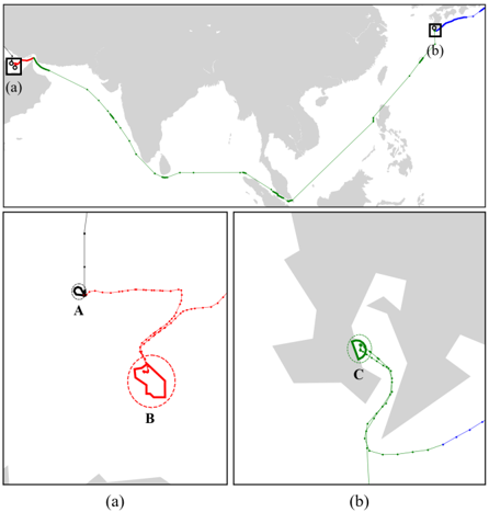
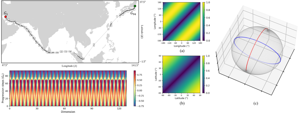
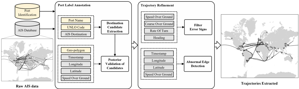
In this work, the port identification dataset and the AIS data are coupled to perform the segmentation and refinement of raw AIS data. The segmentation of portto-port trajectory is conducted along the features from the AIS messages received, by exploiting the DamerauLevenshtein distance [41], [42] and port-wise boundary thresholding, where the detailed implementation is described in Appendix A. Afterward, the segmented port- to-port trajectories undergo the refinement process with the clustering algorithm DBSCAN, of detecting abnormal shifts. The detail of Implementing DBSCAN as verifying the erroneous transmission is depicted in Appendix B. The overall procedure of the data annotating framework is shown in Fig. 1, which illustrates the refined result of 5-year accumulated AIS data from a single vessel.
IV. METHODOLOGY
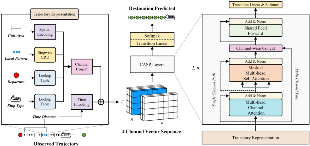
This section presents WAY, the architecture for processing AIS data, with a novel approach toward global trajectory representations. In addition, Gradient Dropout learning technique is proposed to mitigate the feedback bias issue proportional to the data length while designing a many-to-many training framework. This technique is only applied to the training set and detached for inference. The overall framework of the proposed method is illustrated in Fig. 2, where C denotes channels, N implies the number of grid areas observed, d is the hidden dimension size of the model, and L indicates the number of layers repeated as a stack, and WAY is shown to process the trajectories based on 4-channel vector sequences.
A. Trajectory Representation
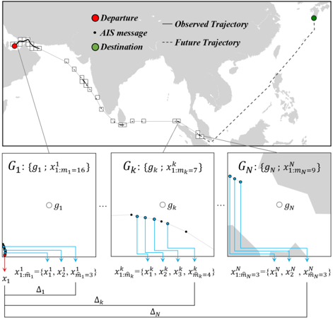
An observed trajectory is processed within each unit area in the WAY architecture. To do so, the raw observations are reconstructed and handled by nature before the main process began. Let us denote x 1: T = { x 1 , . . . , x T } ∈ R T × f as a sequence of AIS observations from an ongoing ship at time step T , where f indicates the number of AIS fields used as features that contain timestamps, longitudes, latitudes, etc. The given sequence can therefore be reorganized using uniform spatial grids to { G 1 , . . . , G N } , where each grid element G k = { g k ; x k 1: m k } for k ∈ { 1 , . . . , N } includes the identity coordinate g k and a subset of observations inside x k 1: m k = { x j +1 , . . . , x j + m k } ⊂ x 1: T , and where j = ∑ k -1 i =1 m i and T = ∑ N i =1 m i .
Thereafter, samples of ˆ m k observations are taken dynamically from x k 1: m k , where ˆ m k follow a Poisson distribution with the parameter λ = 5 . The intention of sampling is to reflect the circumstances under irregular
intervals and consider any moment of trajectory progression when and wherever the observation possibly exists in regions. In addition, sampling can moderate the flooding of redundant AIS records generated by such intervals and also by the reason owing to the timing issue between transmission and receiving. Thus, a subsequential trajectory x k 1: m k ← ˆ m k is redefined by the sampled observations in each G k .
An example of this rearrangement is visualized in Fig. 3, while the longitude, latitude, and timestamp fields included in x k 1: m k are transformed into a manner of relativeness to each grid area belonged. Based on each grid center coordinate g k = ( λ, ϕ ) , the observed longitudes and latitudes ( λ i , ϕ i ) ∈ x k i for i ∈ { 1 , ..., m k } are converted into ( λ -λ i , ϕ -ϕ i ) , and the m k timestamps are converted into m k time distances, measuring the progression in days from the 0 distance for the first sample x k 1 . The trajectory contains the non-sequential features as well, acknowledged from the annotation and the ship itself, which are the departure port Y x and vessel type S x , respectively. Subsequently, the organized model input x = { G 1: N ; Y x ; S x } is handled in the representation layer by each feature component, as described below:
Description of AIS trajectory components
- Unit Area. A sequence of center coordinate ( λ, ϕ ) tuples of the spatial grid from the observed, denoted by { g 1 , ..., g N } ∈ R N × ( λ,ϕ ) .
- Local Pattern. A sequence of subsets from the observed; each includes kinetic patterns corresponding to the unit area. The sequence is denoted by { x 1 1: m 1 , . . . , x N 1: m N } ∈ R N × M × f , where M denotes a set of subsequential lengths.
- Departure. A categorical value of ports Y x ∈ N .
- Ship Type. A categorical value of ships S x ∈ N .
- Time Distance. A sequence of time intervals between each last observation in subsets and the very first from the trajectory, denoted by { ∆ 1 , . . . , ∆ N } ∈ R N where ∆ N = time ∆ ( x N m N -x 1 ) and the intervals are measured in days.
1. Spatial Encoding
Inspired by positional encoding from Transformer [40], Spatial Encoding (SE) module is designed to transform real-valued coordinates into high-dimensional vectors. Given an N observed sequence of the unit area coordinates x ∈ R N × ( λ,ϕ ) and hidden size d , the module produces the output vector sequence x ∈ R N × d as follows:
where the function g( q, 4 i ) = q/ (2 π ) 4 i/d 2 operates with radian unit ( λ, ϕ ) , and i specifies the dimension. The combinations of the sinusoidal functions are motivated by the conversion definition of polar to Cartesian coordinate system, and the frequency from the division term of function g ( q, 4 i ) is set to 2 π . Therefore, the produced vector comprises the sinusoidal wave of marginally different frequencies, where each 4 i th and 4 i + 2 th dimensions are based on the wavelengths from π to π · (2 π ) -1 /d , and 4 i +1 th and 4 i +3 th dimensions corresponds to the wavelengths from 2 π to (2 π ) 1 -1 /d . Fig. 4 illustrates the actual output of the SE module with d = 128 , given the sequence of the grid coordinates from the example trajectory. Fig. 5a and Fig. 5b show the scaled distance distributions between the encoded vectors from sets of each longitudeand latitude-wise sampled coordinates, respectively. As the transformed representations have the cyclic distance with the longitudes and represent the diverging distance distribution with the latitudes, the set of outputs from SE module preserves the spatial distance concept of the original coordinates. As a result, the encoded vector from each grid coordinate represents its own positional identity on the spherical surface, which can
Fig. 5. An example of Spatial Encoding result. (a) indicates the longitude-wise Euclidean distances between encoded vectors, (b) is the distance between vectors arranged in latitudes, and (c) visualizes the 3-dimensional PCA result of encoded vectors ∈ R d from the whole 1 × 1 ( ◦ 2 ) grids, where the Blue are sampled in (a) and Red as (b).
be explained by the dimensionality reduction of Principal Component Analysis (PCA) [43] (see Fig. 5c).
2. Step-wise Gated Recurrent Unit
To capture the ship's behavioral details and specify local patterns in uniform grid areas, Gated Recurrent Unit (GRU) [44] is used to process each subsequence, which employs the concept of LSTM, updating hidden and cell states via gate functions while using fewer parameters. Given the individual subsequence x k ∈ R m k × f , the state update at the current step t ∈ [1 , . . . , m k ] is defined by the input x k t , sigmoid function σ , update gate u t , and reset gate r t , as follows:
Batchifying the process among the N sequence steps, each input subsequence x k ∈ R m k × f yields h m k ∈ R d using the ( L/ 2 )-layered GRU stack. Consequently, the set of last hidden states [ h m 1 ; . . . ; h m N ] ∈ R N × d represents the sequence of local navigational patterns.
3. Semantic Representations and Time Encoding
Objectifying a port-to-port trajectory as a single analytic instance, departure and vessel types contain a semantic relationship toward the port destination. That is, international shipments do not occur randomly, but are involved in national trading relations, goods, and needs. Learnable parameters are set for Y worldwide ports and S types of ships such that each lookup table can be described by W Y ∈ R Y × d and W S ∈ R S × d , respectively. The tables return the vectors of W Y x ∈ R d and W S x ∈ R d indexed by departure Y x and ship type S x .
Thereafter, the vectors are sequentialised by adding time information in order. Modifying positional encoding [40], Time Encoding (TE) module generates representations of the temporal progression of a given trajectory. Whereas the fixed uniform-discrete offset is given to the original encoding procedure, AIS data comprises the sequence of irregular intervals. Therefore the procedure has to be adjusted to accept a real-value offset input ∆ , the day-unit time distance, and operate as a continuous function. Based on the timestamps of each sampled subsequence as shown in Fig. 3, given the time distances between the last samples and the first observation of whole trajectory, the equation to process input x ∈ R N can be defined as:
where i specifies the dimension. To sufficiently cover the maximum temporal progression of the vessel operations and consider the adequate intervals within the encoded representations, the frequency of the sinusoidal functions in TE is set to 1000. Subsequently, the TE output is produced as x ∈ R N × d , forming a geometric progression in each dimension based on wavelengths from 2 π to 1000 · 2 π . The sequence of time-encoded vectors is added to W Y x and W S x each while duplicating their identical for N steps, as well as to the sequence outputs that were defined from Sec. IVA1 and Sec. IVA2 each. Accordingly, the concatenation of such representations yields a 4-channel vector sequence x ∈ R C × N × d , where C = 4 . An observed AIS trajectory is time-sequentially depicted by perspectives of global space, local patterns, and semantics in the respective channels.
B. Channel Aggregative Sequence Processing
Based on the multi-channel vector sequence output from the representation layer, Channel Aggregative Sequence Processing (CASP) layer is proposed to aggregate each distinct nature of AIS data distributed over channels and convey the sequential information toward the current step of the decision. CASP layer comprises multi-head channel attention (MCA), masked multi-head self-attention (MSA), and shared feed-forward (SFF) network modules responsible for current feature aggregation, sequential processing, and decoding, respectively.
1. Multi-head Channel Attention
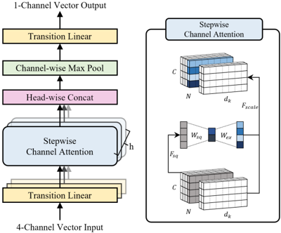
Channel Attention was first proposed in the Squeezeand-Excitation network [45] in the computer vision domain. This method involves conducting an information comparison among channels and emphasizing each by the compared results. The concept is extended in WAY to a multi-perspective comparison by applying an identical set of linear transitions to channels, as shown in Fig. 6. MCA aggregates the current step representations from each channel into a single vector comprising accentuated dimensions. From individual steps x ∈ R C × d , the per-
spectives are spread via W tr i ∈ R d × d k for i ∈ [1 , . . . , h ] , where h denotes the number of heads and d k is dimensions per head. Thus, the current step x ∈ R h × C × d k is given, and the equation of multi-headed attention is as follows:
where F AVG sq is the average pooling function and F AVG sq is the max pooling in terms of dimensions in each channel. The squeezed z avg , z max ∈ R h × C is transformed into the corresponding z ′ avg , z ′ max ∈ R h × C using the shared parameters W sq and W ex . The procedures for each head are performed in parallel using W sq ∈ R h × C × C/γ and W ex ∈ R h × C/γ × C , where γ = 2 and ReLU [46] activation is applied to the bottleneck. The attention weight α C ∈ R h × C emphasizes the channels of the input x , where the sigmoid function σ contracts the sum of the intensities in the range of (0 , 1) . The emphasized tensor ˜ x ∈ R h × C × d k are transposed to ˜ x ∈ R C × ( h · d k ) by headwise concatenation and then a max pooling function is applied over channels, extracting the most highlighted values for each dimension. Thereby 1-channel vector output ˜ x ∈ R ( h · d k ) is provided, and the final result of the module ˜ x ∈ R d is produced by the linear transition of W out ∈ R ( h · d k ) × d . Considering that aggregation occurs at every step, the sequence output from the MCA module is denoted by x ∈ R N × d .
2. Masked Multi-head Self Attention
Originally introduced to address the neural machine translation problem, Transformer [40] has further improved the performance of deep learning approaches in several domains, and this method has been widely used in state-of-the-art studies. The proposed concept of selfattention maximizes the utilization of attention mechanisms [47], [48], capturing long-term correlations in given sequential data. In WAY, the transformer decoder archi-
tecture is adopted to convey past trajectory representations toward the current step and decode such information into features for destination estimation.
With the proceeded output x ∈ R N × d from the fore MCA module, MSA delivers the past aggregated information to the present. The multi-headed attention weight α S ∈ R h × N × N is defined by the following equations:
where i ∈ [1 , . . . , h ] indicates each head, d k denotes the head dimension, and Q,K, and V ∈ R h × N × d k are the sets of vectors transformed by W Q i , W i K , and W V i ∈ R d × d k , respectively. Based on the matrix multiplication of Q and K T ∈ R h × d k × N , the inter-correlation scores are measured over sequence steps, and the lower triangular matrix filter F mask is applied to block information flows from future steps. Thus, α S is given, and ˜ V ∈ R h × N × d k is produced, of which the vectors in V are scaled and mixed with the representations from the past. Eventually, the concatenation of the heads ˜ V ∈ R N × ( h · d k ) is multiplied by a linear transition W out ∈ R ( h · d k ) × d , providing the output sequence ˜ V ∈ R N × d .
3. Channel Concatenation and Shared Feed Forward
Before applying SFF module procedure, the channelwise concatenation between the original CASP layer input sequence x ∈ R C × N × d and the output sequence x ∈ R N × d from MSA module proceeds. The concatenation, which is more likely to be said to substitute a certain channel sequence, is to withdraw one of the channels from the original input and fill the spot with the output of MSA module. Despite the replacement, the altered channel has more enriched information and incorporates the withdrawn identity because of the residual connections that will be described in Sec. IVB4. In this study, the single channel is designated to be repeatedly replaced over the stack of CASP layers in the procedure, that is, the output from SE module. The purpose of the design is to update a certain channel by gathering all channel-wise features and sequential information, whereas the others maintain their current step identities. Based on the idea of CSPNet [49], the connection not only relieves the computational burden, but also gives the model the ability to add up representations enriched repeatedly within the stack of CASP layers.
Consequently, the concatenated tensor x ∈ R C × N × d maintains the number of channels C , and SFF module performs linear transformations for each representation in a given tensor. The module comprises 2-layered fully connected network W 1 ∈ R d × d f and W 2 ∈ R d f × d with intermediate ReLU activation, as the transition is shared in positions and channels. Accordingly, CASP layer output x ∈ R C × N × d can be obtained.
4. Residual Connection
As shown in Fig. 2, residual connection [50] and layer normalization [51] follow each submodule in CASP layer. The residual connection adds input x to the output from the module, which is presented to address the vanishing gradient problem of deep neural network architectures. Layer normalization is used to stabilize the hidden state dynamics in the sequential modeling. As introduced in [40], the same combination is applied to MSA and SFF, where the inputs and outputs of each have identical shapes. However, in the MCA module, where channels are aggregated and the output comprises a single channel, only the designated input channel is subjected to such an architecture. Considering that a certain channel was designated to be replaced in Sec. IVB3, the channel to be withdrawn preserves its identity through residual connection, and moreover, it reflects the aggregated representation over both channels and sequence since MSA proceeds the output sequence from MCA module.
C. Loss Function and Learning Technique
In this study, the classification problem of destination estimation is formulated given the vessel trajectory from its departure. Therefore, let the model input be denoted as x = { x 1 , . . . , x T ; Y x ; S x } , where an accumulated AIS observation from a single ongoing ship at time step T and the voyage is departed from port Y x and the ship belongs to type S x . Thereafter, in processing the multichannel sequence structure, WAY repeatedly aggregates information from channels and the past. The current step of the designated channel representation x ∈ R d is converted from the last CASP block output to a probability distribution over port classes using the final linear transition W ∈ R d × Y with the softmax function, which is defined as:
where CE denotes Cross Entropy loss, y ∈ Y is the future destination port, and θ denotes the model parameters.
Indeed, by exploiting the loss above, a many-to-many model training framework results in a biased parameter update. Given the full port-to-port trajectories, the summation of feedback within the sequence toward a single destination can be affected by certain extremely long instances. To address this issue, Gradient Dropout learning technique is proposed. This technique controls the validity of stepwise loss from each instance in the mini-batch. The validity is determined stochastically by the sampling ratio, which is inversely proportional to the log-scaled length of the instances, as follows:
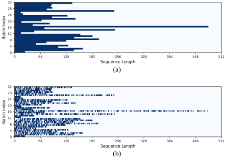
where N k for k ∈ { 1 , . . . , B } denotes the length of the k th among B instances in the mini-batch. As shown in Fig. 7, sampling ratio δ k adjusts the feedback validity over instances, balancing the loss update against the lengths.
D
V. EXPERIMENTS
A. Dataset
Satellite AIS data collected from ORBCOMM and port identification data provided by SeaVantage were used during this study. Experiments were conducted on 5year (January 2016-November 2020) accumulated realworld AIS data of 5,103 individual ships, where the vessels belong to one of three types: tanker, container, and bulk. A total of ≃ 130 K trajectories comprising ≃ 17 M AIS messages were mapped between 3,243 port classes using the framework described in Section IIIB. A destination-wise stratified split was used to generate the training/validation/test trajectory dataset as 70% , 15% , and 15% of the total.
Given AIS trajectory instances, the features exploited by the proposed method are listed in Table I. In addition to the timestamps and coordinates, relevant to the preprocessing of the relative coordinates and time distances previously stated in Sec. IVA, other numerical features were adopted to reflect the local navigational patterns. It should also be noted that ETA, which is human-generated, was preprocessed to the time distance between the current timestamp, and the departure port indicates the categorical index among the list of total port classes.
B. Experimental Setup
1. Benchmark Models and Implementation Details
Benchmark models selected from previous studies were employed to process AIS data, and the details were modified to meet the objective of the task. LSTM [38] was the most frequently used sequence model in the maritime domain. Sharing the gated sequential processing concept with LSTM, GRU [44] was occasionally adopted as a comparison in priors and the applications of the attention mechanism [48] to both LSTM and GRU were also considered. In addition, considering that Transformer [40] has improved the performance of various sequential data
| Category | Features | Unit |
|---|---|---|
| AIS | Timestamp Estimated Time of Arrival Longitude Latitude Speed Over Ground Rate Of Turn Course Over Ground Heading AIS draught Ship Type | UTC UTC degree degree knot degree degree degree meter categorical |
| Port | Departure | categorical |
processing fields, Transformer-decoder and TrAISformer [12] architectures were added for comparison.
Dividing the global ocean area into a spatial grid, a unit size of 1 × 1 ( ◦ 2 ) was set as the processing unit. As a contemplation of prior grid-token-based approaches, the comparison models embedded lookup tables for spatial vocabularies and learned their representations from the training set. In the comparison of benchmarks, the models shared the hyperparameters of the number of stacked layers L = 4 and hidden dimension size d = 128 . In addition, TrAISformers, Transformer-decoder, and WAY shared the hyperparameters relevant to the attention architecture and feedforward network, which are the number of attention heads h = 4 , the head-wise hidden dimension size d k = 64 , and the intermediate dimension size in the feedforward network d f = 256 . The models were trained using the Adam [52] optimizer for 100 epochs with a batch size of 32 and dropout ratio of 30% , where the learning rate was set to 1 e -4 . Test evaluations were conducted for each model when the minimal loss was recorded for the validation set.
2. Evaluation Metric
An accuracy metric was adopted to evaluate the models in terms of port classification, where the overall and quartile-based accuracies were measured. The overall accuracy subjectifies the correctness of the model's estimation for every grid-unit step. The evaluation of accuracy is measured as the equation below:
✶ where i indexes the trajectory instances from the test set M , and N i corresponds to the length of unit-grid sequence composing the i th instance. The destination port class of i th trajectory is denoted by y i , and ˆ y ij indicates the class of the maximum probability the model infers at the progression step j of the trajectory. Given that the performance can vary depending on the voyage progress, the accuracy of different voyage progressions was also assessed. Quartile-based accuracy was measured by adjusting the iteration range of j from Equation 14. The models were
| Method | Accuracy(%) | F1-score(%) | ||||
|---|---|---|---|---|---|---|
| Overall | 0Q ∽ 1Q | 1Q ∽ 2Q | 2Q ∽ 3Q | 3Q ∽ 4Q | Overall | |
| LSTM | 56.48 ± 0.32 | 40.90 ± 0.60 | 56.63 ± 0.16 | 62.48 ± 0.27 | 67.04 ± 0.49 | 27.30 ± 1.22 |
| LSTM-ATTN | 55.76 ± 0.17 | 41.60 ± 0.15 | 55.77 ± 0.35 | 61.56 ± 0.35 | 65.13 ± 0.23 | 27.40 ± 0.82 |
| GRU | 56.35 ± 0.40 | 41.30 ± 0.07 | 55.74 ± 0.55 | 62.18 ± 0.50 | 67.25 ± 0.52 | 29.02 ± 0.11 |
| GRU-ATTN | 56.45 ± 0.09 | 41.54 ± 0.26 | 56.32 ± 0.39 | 62.25 ± 0.16 | 66.60 ± 0.21 | 28.21 ± 0.15 |
| Transformer-decoder | 60.26 ± 0.05 | 44.35 ± 0.26 | 59.45 ± 0.27 | 65.83 ± 0.32 | 72.46 ± 0.12 | 32.79 ± 0.53 |
| TrAISformer | 64.38 ± 0.14 | 50.15 ± 0.22 | 63.62 ± 0.10 | 69.44 ± 0.12 | 75.27 ± 0.13 | 33.12 ± 0.26 |
| TrAISformer-multiResolution | 64.60 ± 0.28 | 50.23 ± 0.36 | 64.07 ± 0.49 | 69.60 ± 0.22 | 75.46 ± 0.13 | 34.10 ± 0.26 |
| WAY (ours) | 79.45 ± 0.32 | 71.21 ± 0.21 | 79.50 ± 0.22 | 82.42 ± 0.40 | 85.25 ± 0.47 | 49.45 ± 0.68 |
| WAY w/ GD (ours) | 80.44 ± 0.11 | 71.96 ± 0.20 | 80.19 ± 0.14 | 83.38 ± 0.06 | 86.81 ± 0.20 | 52.01 ± 0.80 |
evaluated along the quarter-wise accumulated progression of each test trajectory, hence the range of (1 , N i ) at the term ∑ N i j =1 was adjusted into (1 , 1 4 N i ) , ( 1 4 N i +1 , 1 2 N i ) , ( 1 2 N i +1 , 3 4 N i ) , and ( 3 4 N i +1 , N i ) , according to quartiles respectively.
Additionally, an overall F1-score was adopted to verify the models under an imbalanced label condition. The measurement of F1-score for each port class c follows the equation below: