A Linear Time Natural Evolution Strategy for Non-Separable Functions

Yi Sun, Faustino Gomez, Tom Schaul, and J¨ urgen Schmidhuber

IDSIA, University of Lugano & SUPSI, Galleria 2, Manno, CH-6928, Switzerland yi,tino,tom,juergen @idsia.ch

{ }

Abstract. We present a novel Natural Evolution Strategy (NES) variant, the Rank-One NES (R1-NES), which uses a low rank approximation of the search distribution covariance matrix. The algorithm allows computation of the natural gradient with cost linear in the dimensionality of the parameter space, and excels in solving high-dimensional nonseparable problems, including the best result to date on the Rosenbrock function (512 dimensions).

1 Introduction

Black-box optimization (also called zero-order optimization) methods have received a great deal of attention in recent years due to their broad applicability to real world problems [7,9-11,15,18]. When the structure of the objective function is unknown or too complex to model directly, or when gradient information is unavailable or unreliable, such methods are often seen as the last resort because all they require is that the objective function can be evaluated at specific points.

In continuous black-box optimization problems, the state-of-the-art algorithms, such as xNES [4] and CMA-ES [8], are all based the same principle [1,4]: a Gaussian search distribution is repeatedly updated based on the objective function values of sampled points. Usually the full covariance matrix of the distribution is updated, allowing the algorithm to adapt the size and shape of the Gaussian to the local characteristics of the objective function. Full parameterization also provides invariance under affine transformations of the coordinate system, so that ill-shaped, highly non-separable problems can be tackled. However, this generality comes with a price. The number of parameters scales quadratically in the number of dimensions, and the computational cost per sample is at least quadratic in the number of dimensions [13], and sometimes cubic [4,16].

This cost is often justified since evaluating the objective function can dominate the computation, and thus the main focus is on the improvement of sampling efficiency. However, there are many problems, such as optimizing weights in neural networks where the dimensionality of the parameter space can be very large (e.g. many thousands of weights), the quadratic cost of updating the search distribution can become the computational bottleneck. One possible remedy is to restrict the covariance matrix to be diagonal [14], which reduces the computation per function evaluation to O ( d ), linear in the number d of dimensions.

Unfortunately, this 'diagonal' approach performs poorly when the problem is non-separable because the search distribution cannot follow directions that are not parallel to the current coordinate axes.

In this paper, we propose a new variant of the natural evolution strategy family [17], termed Rank One NES (R1-NES). This algorithm stays within the general NES framework in that the search distribution is adjusted according to the natural gradient [2], but it uses a novel parameterization of the covariance matrix, where u and σ are the parameters to be adjusted. This parameterization allows the predominant eigen direction, u , of C to be aligned in any direction, enabling the algorithm to tackle highly non-separable problems while maintaining only O ( d ) parameters. We show through rigorous derivation that the natural gradient can also be effectively computed in O ( d ) per sample. R1-NES scales well to high dimensions, and dramatically outperforms diagonal covariance matrix algorithms on non-separable objective functions. As an example, R1-NES reliably solves the the non-convex Rosenbrock function up to 512 dimensions.

The rest of the paper is organized as follows. Sectio 2, briefly reviews the NES framework. The derivation of R1-NES is presented in Section 3. Section 4 empirically evaluates the algorithm on standard benchmark functions, and Section 5 concludes the paper.

2 The NES framework

Natural evolution strategies (NES) are a class of evolutionary algorithms for real-valued optimization that maintain a search distribution, and adapt the distribution parameters by following the natural gradient of the expected function value. The success of such algorithms is largely attributed to the use of natural gradient, which has the advantage of always pointing in the direction of the steepest ascent, even if the parameter space is not Euclidean. Moreover, compared to regular gradient, natural gradient reduces the weights of gradient components with higher uncertainty, therefore making the update more reliable. As a consequence, NES algorithms can effectively cope with objective functions with ill-shaped landscapes, especially preventing premature convergence on plateaus and avoiding overaggressive steps on ridges [16].

The general framework of NES is given as follows: At each time step, the algorithm samples n ∈ N new samples x 1 , . . . , x n ∼ π ( ·| θ ), with π ( ·| θ ) being the search distribution parameterized by θ . Let f : R d ↦→ R be the objective function to maximize. The expected function value under the search distribution is

Using the log-likelihood trick, the gradient w.r.t. the parameters can be written as

from which we obtain the Monte-Carlo estimate

of the search gradient. The key step of NES then consists of replacing this gradient by the natural gradient

where is the Fisher information matrix (See Fig.1 for an illustration). This leads to a straightforward scheme of natural gradient ascent for iteratively updating the parameters

The sequence of 1) sampling an offspring population, 2) computing the corresponding Monte Carlo estimate of the gradient, 3) transforming it into the natural gradient, and 4) updating the search distribution, constitutes one iteration of NES.

The most difficult step in NES is the computation of the Fisher information matrix with respect to the parameterization. For full Gaussian distribution, the Fisher can be derived analytically [4,16]. However, for arbitrary parameterization of C , the Fisher matrix can be highly non-trivial.

3 Natural gradient of the rank-one covariance matrix approximation

In this paper, we consider a special formulation of the covariance matrix

with parameter set θ = 〈 σ, u 〉 . The special part of the parameterization is the vector u ∈ R d , which corresponds to the predominant direction of C . This allows the search distribution to be aligned in any direction by adjusting u , enabling the algorithm to follow valleys not aligned with the current coordinate axes, which is essential for solving non-separable problems.

Since σ should always be positive, following the same procedure in [4], we parameterize σ = e λ , so that λ ∈ R can be adjusted freely using gradient descent without worrying about σ becoming negative. The parameter set is adjusted to θ = 〈 λ, u 〉 accordingly.

From the derivation of [16], the natural gradient on the sample mean is given by

In the subsequent discussion we always assume µ = 0 for simplicity. It is straightforward to sample from N (0 , C ) 1 by lettting y ∼ N (0 , I ), z ∼ N (0 , 1), then

The inverse of C can also be computed easily as where r 2 = u glyph[latticetop] u . Using the relation det ( I + uu glyph[latticetop] ) = 1 + u glyph[latticetop] u , the determinant of C is

Knowing C -and | C | allows the log-likelihood to be written explicitly as

The regular gradient with respect to λ and u can then be computed as:

Replacing x with e λ ( y + zu ), then the Fisher can be computed by marginalizing out i.i.d. standard Gaussian variables y and z , namely,

1 For succinctness, we always assume the mean of the search distribution is 0. This can be achieved easily by shifting the coordinates.

Since elements in glyph[triangleinv] θ log p ( x | θ ) glyph[triangleinv] θ log p ( x | θ ) glyph[latticetop] are essentially polynomials of y and z , their expectations can be computed analytically 2 , which gives the exact Fisher information matrix with

Let v = u/r , then

The inverse of F is thus given by

We apply the formula for block matrix inverse in [12]

where C 1 = A 11 -A 12 A -22 A 21 , and C 2 = A 22 -A 21 A -11 A 12 are the Schur complements. Let F be partitioned as above, then

and the Shur complements are

and

2 The derivation is tedious, thus omitted here. All derivations are numerically verified using Monte-Carlo simulation.

whose inverse is given by and

Note that computing both ˜ glyph[triangleinv] λ log p ( x | θ ) and ˜ glyph[triangleinv] u log p ( x | θ ) requires only the inner products x glyph[latticetop] x and x glyph[latticetop] v , therefore can be done O ( d ) storage and time.

3.1 Reparameterization

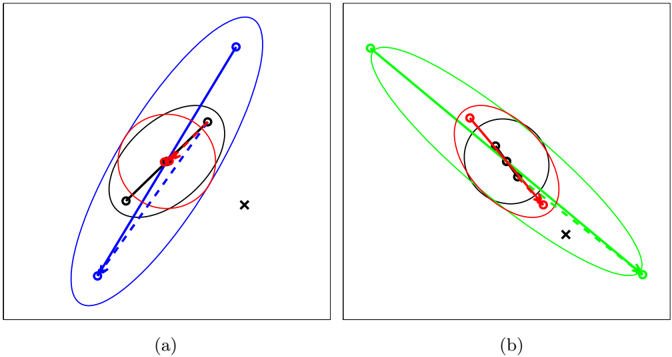
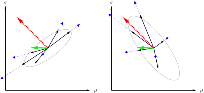
The natural gradient above is obtained with respect to u . However, direct gradient update on u has an unpleasant property when ˜ glyph[triangleinv] u log p ( x | θ ) is in the opposite direction of u , which is illustrated in Fig. 2(a). In this case, the gradient tends to shrink u . However, if ˜ glyph[triangleinv] u log p ( x | θ ) is large, adding the gradient will flip the direction of u , and the length of u might even grow. This causes numerical problems, especially when r is small. A remedy is to separate the length and direction of u , namely, reparameterize u = e c v , where ‖ v ‖ = 1 and e c is the length of u . Then the gradient update on c will never flip u , and thus avoid the problem.

Note that for small change δu , the update on c and v can be obtained from

Combining the results gives the analytical solution of the inverse Fisher:

Multiplying F -with the regular gradient in Eq.3 and Eq.4 gives the natural gradient for λ and u :

Algorithm 1: R1-NES( n )

1 while not terminate do 2 for i = 1 to n do 3 y i ←N (0 , I ) 4 z i ←N (0 , 1) 5 x i ← e λ ( y i + z i u ) //generate sample 6 fitness[i] ← f ( µ + x i ) 7 end 8 Compute the natural gradient for µ , λ , u , c , and v according to Eq.2, 5, 6, 7, and 8, and combine them using Eq.1 9 µ ← µ + η ˜ glyph[triangleinv] µ J 10 λ ← λ + η ˜ glyph[triangleinv] λ J 11 if ˜ glyph[triangleinv] c log p ( x | θ ) < 0 then 12 c ← c + η ˜ glyph[triangleinv] c J 13 v ← v + η ˜ glyph[triangleinv] v J ‖ v + η ˜ glyph[triangleinv] v J ‖ 14 u ← e c v 15 else 16 u ← u + η ˜ glyph[triangleinv] u J //additive update 17 c ← log ‖ u ‖ 18 v ← u ‖ u ‖ 19 end 20 end

and

The natural gradient on c and v is given by letting δu ∝ ˜ glyph[triangleinv] u log p ( x | θ ), thanks to the invariance property:

Note that computing ˜ glyph[triangleinv] c log p ( x | θ ) and ˜ glyph[triangleinv] v log p ( x | θ ) involves only inner products between vectors, which can also be done linearly in the number of dimensions.

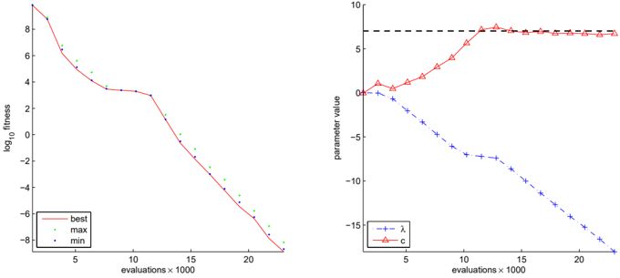
Using the parameterization 〈 c, v 〉 introduces another problem. When r is small, ˜ glyph[triangleinv] c log p ( x | θ ) tends to be large, and thus directly updating c causes r to grow exponentially, resulting in numerical instability, as shown in Fig. 2(b). In this case, the additive update on u , rather than the update on 〈 c, v 〉 is more stable. In our implementation, the additive update on u is used if ˜ glyph[triangleinv] c log p ( x | θ ) > 0, otherwise the update is on 〈 c, v 〉 . This solution proved to be numerially stable in all our tests. Algorithm 1 shows the complete R1-NES algorithm in pseudocode.

4 Experiments

The R1-NES algorithm was evaluated on the twelve noise-free unimodal functions [6] in the 'Black-Box Optimization Benchmarking' collection (BBOB) from the 2010 GECCO Workshop for Real-Parameter Optimization. In order to make the results comparable those of other methods, the setup in [5] was used, which transforms the pure benchmark functions to make the parameters non-separable (for some) and avoid trivial optima at the origin.

R1-NES was compared to xNES [3], SNES [14] on each benchmark with problem dimensions d = 2 k , k = { 1 .. 9 } (20 runs for each setup), except for xNES, which was only run up k = 6 , d = 64. Note that xNES serves as a proper baseline since it is state-of-the-art, achieving performance on par with the popular CMA-ES. The reference machine is an Intel Core i7 processor with 1.6GHz and 4GB of RAM.

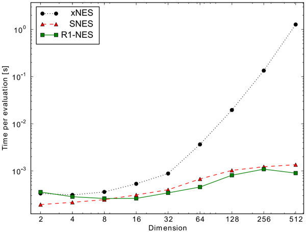
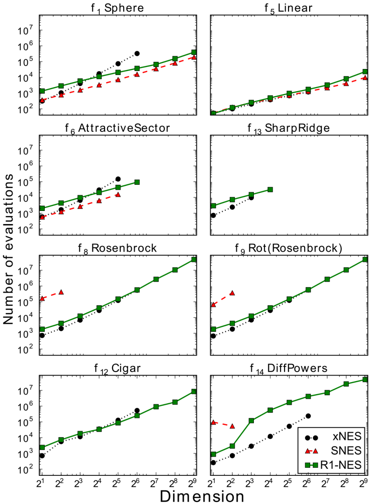
Fig. 3 shows the results for the eight benchmarks on which R1-NES performs at least as well as the other methods, and often much better. For dimensionality under 64, R1-NES is comparable to xNES in terms of the number of fitness evaluations, indicating that the rank-one parameterization of the search distribution effectively captures the local curvature of the fitness function (see Fig.5 for example). However, the time required to compute the update for the two algorithms differs drastically, as depicted in Fig. 4. For example, a typical run of xNES in 64 dimensions takes hours (hence the truncated xNES curves in all graphs), compared to minutes for R1-NES. As a result, R1-NES can solve these problems up to 512 dimensions in acceptable time. In particular, the result on the 512-dimensional Rosenbrock function is, to our knowledge, the best to date. We estimate that optimizing the 512-dimensional sphere function with xNES (or any other full parameterization method, e.g. CMA-ES) would take over a year in computation time on the same reference hardware. It is also worth pointing out that sNES, though sharing similar, low complexity per function evaluation, can only solve separable problems (Sphere, Linear, AttractiveSector, and Ellipsoid).

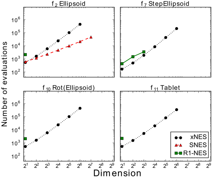
Fig. 6 shows four cases (Ellipsoid, StepEllipsoid, RotatedEllipsoid, and Tablet) for which R1-NES is not suited, highlighting a limitation of the algorithm. Three of the four functions are from the Ellipsoid family, where the fitness functions are variants of the type

The eigenvalues of the Hessian span several orders of magnitude, and the parameterization with a single predominant direction is not enough to approximate the Hessian, resulting in poor performance. The other function where R1-NES fails is the Tablet function where all but a one eigendirection has a large eigenvalue. Since the parameterization of R1-NES only allows a single direction to have a large eigenvalue, the shape of the Hessian cannot be effectively approximated.

5 Conclusion and future work

We presented a new black-box optimization algorithm R1-NES that employs a novel parameterization of the search distribution covariance matrix which allows a predominant search direction to be adjusted using the natural gradient with complexity linear in the dimensionality. The algorithm shows excellent performance in a number of high-dimensional non-separable problems that, to date, have not been solved with other parameterizations of similar complexity.

Future work will concentrate on overcoming the limitations of the algorithm (shown in Fig 6). In particular, we intend to extend the algorithm to a) incorporate multiple search directions, and b) enable each search direction to shrink as well as grow.

Acknowledgement

This research was funded in part by Swiss National Science Foundation grants 200020-122124, 200020-125038, and EU IM-CLeVeR project (#231722).

References

1. Y. Akimoto, Y. Nagata, I. Ono, and S. Kobayashi. Bidirectional Relation between CMA Evolution Strategies and Natural Evolution Strategies. In Parallel Problem Solving from Nature (PPSN) , 2010.
2. S. Amari. Natural gradient works efficiently in learning. Neural Computation , 10(2):251-276, 1998.
3. T. Glasmachers, T. Schaul, Y. Sun, D. Wierstra, and J. Schmidhuber. Exponential Natural Evolution Strategies. In Genetic and Evolutionary Computation Conference (GECCO) , Portland, OR, 2010.
4. T. Glasmaches, T. Schaul, Y. Sun, and J. Schmidhuber. Exponential natural evolution strategies. In GECCO'10 , 2010.
5. N. Hansen and A. Auger. Real-parameter black-box optimization benchmarking 2010: Experimental setup, 2010.
6. N. Hansen and S. Finck. Real-parameter black-box optimization benchmarking 2010: Noiseless functions definitions, 2010.
7. N. Hansen, A. S. P. Niederberger, L. Guzzella, and P. Koumoutsakos. A method for handling uncertainty in evolutionary optimization with an application to feedback control of combustion. Trans. Evol. Comp , 13:180-197, 2009.
8. N. Hansen and A. Ostermeier. Completely derandomized self-adaptation in evolution strategies. Evolutionary Computation , 9(2):159-195, 2001.
9. M. Hasenj¨ ager, B. Sendhoff, T. Sonoda, and T. Arima. Three dimensional evolutionary aerodynamic design optimization with CMA-ES. In Proceedings of the 2005 conference on Genetic and evolutionary computation , GECCO '05, pages 2173-2180, New York, NY, USA, 2005. ACM.
10. M. Jebalia, A. Auger, M. Schoenauer, F. James, and M. Postel. Identification of the isotherm function in chromatography using cma-es. In IEEE Congress on Evolutionary Computation , pages 4289-4296, 2007.
11. J. Klockgether and H. P. Schwefel. Two-phase nozzle and hollow core jet experiments. In Proc. 11th Symp. Engineering Aspects of Magnetohydrodynamics , pages 141-148, 1970.
12. K. B. Petersen and M. S. Pedersen. The matrix cookbook, 2008.
13. R. Ros and N. Hansen. A Simple Modification in CMA-ES Achieving Linear Time and Space Complexity. In R. et al., editor, Parallel Problem Solving from Nature, PPSN X , pages 296-305. Springer, 2008.
14. T. Schaul, T. Glasmachers, and J. Schmidhuber. High Dimensions and Heavy Tails for Natural Evolution Strategies. In To appear in: Genetic and Evolutionary Computation Conference (GECCO) , 2011.
15. O. M. Shir and T. B¨ ack. The second harmonic generation case-study as a gateway for es to quantum control problems. In Proceedings of the 9th annual conference on Genetic and evolutionary computation , GECCO '07, pages 713-721, New York, NY, USA, 2007. ACM.
16. Y. Sun, D. Wierstra, T. Schaul, and J. Schmidhuber. Stochastic search using the natural gradient. In ICML'09 , 2009.
17. D. Wierstra, T. Schaul, J. Peters, and J. Schmidhuber. Natural Evolution Strategies. In Proceedings of the Congress on Evolutionary Computation (CEC08), Hongkong . IEEE Press, 2008.
18. S. Winter, B. Brendel, and C. Igel. Registration of bone structures in 3d ultrasound and ct data: Comparison of different optimization strategies. International Congress Series , 1281:242 - 247, 2005.

Using the log-likelihood trick, the gradient w.r.t. the parameters can be written as

∫

θ

/triangleinv

∫

E

=

=

=

f

[

f

f

(

(

x

)

(

x

x

)

π

)

π

(

x

/triangleinv

θ

(

x

|

θ

)

log

|

θ

)

/triangleinv

θ

π

π

(

dx

π

(

(

x

x

x

|

θ

from which we obtain the Monte-Carlo estimate

1

n

n

=1

∑

|

θ

θ

)

)

)] ,

|

π

(

x

i

/triangleinv

θ

/triangleinv

J

θ

J

/similarequal

i

f

(

x

i

)

/triangleinv

θ

log dx

|

θ

) .