一

A Possibilistic Model for Qualitative Sequential Decision Problems under Uncertainty in Partially Observable Environments

Regis Sabbadin

IRIT - Universite Paul Sabatier 31062 Toulouse Cedex (France)

e-mail:

sabbadinOiri t. fr

Abstract

In this article we propose a qualitative ( ordi­ nal) counterpart for the Partially Observable Markov Decision Processes rnodel (POMDP) in which the uncertainty, as well as the prefer­ ences of the agent, are modeled by possibility distributions. This qualitative counterpart of the POMDP model relies on a possibilistic theory of decision under uncertainty, recently developed.

counterpart of the Choquet integral generalizing the expected utility criterion. It has received axiomatic justifications in the style of von Neumann and Morgen­ stem [Dubois & Pradel995] and recently in the style of Savage [Dubois, Prade, & Sabbadinl998].

One advantage of such a qualitative frame­ work is its ability to escape from the classi­ cal obstacle of stochastic POMDPs, in which even with a finite state space, the obtained belief state space of the POMDP is infinite. Instead, in the possibilistic framework even if exponentially larger than the state space, the belief state space remains finite.

1 INTRODUCTION

The Partially 0 bservable Markov Decision Processes model (POMDP) is a general model for sequential de­ cision problems in which effects of actions as well as results of observations are noisy, and the noise is rep­ resented by probability distributions.

The POMDP model takes its justification from the most widely used theory for decision under un­ certainty : the expected utility theory [Savagel954] [von Neumann & Morgensternl944). It is theoreti­ cally very attractive but its practical use remains diffi­ cult, especially because it involves infinite state spaces.

In this article we propose an ordinal counterpart of the POMDP model in which uncertainty as well as pref­ erences are modeled by qualitative possibility distri­ butions that take their values in a finite ordinal scale. The underlying decision criterion is based on the use of the Sugeno integral which is an ordinal, maxmin,

In the next section we will describe the usual frame­ work of fully and partially observable markov decision processes as well as some classical resolution meth­ ods. We will recall, in particular, how POMDPs can be restated as fully observable MOPs on the (infinite, continuous) belief state space, thus leading to define methods that approximate the value of optimal poli­ cies, either by updating a value function, or by dis­ cretizing the continuous belief state space.

Then, in section 3 we w i l l give some back­ ground on the possibilistic utility functions advo­ cated by [Dubois & Pradel995], and we will see how [Fargier, Lang, & Sabbadinl998] proposed to extend them to multistage decision making (in a fully ob­ servable domain). In particular, we will recall some decomposability properties that allow to use dynamic programming-like algorithms to solve such possibilis­ tic multistage decision problems (that we call 11MDPs). In [Fargier, Lang, & Sabbadinl998], espe­ cially, a backwards induction algorithm is proposed, for solving finite-horizon 11-MDPs. In the present ar­ ticle, we first give a slightly different version of this algorithm, which makes it similar to the value itera­ tion algorithm used for solving classical MOPs, and allows to handle the infinite horizon as well as the fi­ nite horizon case.

Section 4 is the central part of the paper : here we will recall how conditioning can be defined (not uniquely, by the way) in possibility theory. We will then de­ fine a possibilistic counterpart of POMDPs which, we will show, can be handled by finite domain 11-MDP algorithms, even if considering partial observability in 11-POMDPs makes the computation of optimal poli­ cies exponentially (in space and time) more difficult than in the completely observable case.

2 MARKOV DECISION PROCESSES

2.1 FULLY OBSERVABLE MARKOV DECISION PROCESSES

The standard MDP model [Puterman1994] is defined by :

• A set T C IN of stages in which decisions must be taken. W hen Tis finite (T = {0, . . . N}), N is the horizon of the problem.
• For each stage t, a finite state space, St.
• Sets A, , t (finite) of available actions in state s at stage t (these sets are denoted A, when they do not depend on t).
• The rewards r(s, a) that are obtained after a has been applied in state s. These rewards may be negative, thus considered as costs or penalties.
• To each action a E A, t applied in state s E St is assigned a probabilit � distribution p(· Js, a) de­ scribing the uncertainty about the possible suc­ cessor states in St + l·

A decision rule d1 is an application from St to Uses,As,t assigning an action to each possible state of the world in stage t. The set of these decision rules is denoted by Dt. A policy 8 is, in the finite horizon case, a n-tuple of decision rules 8 = (d1 , ... , dN) where N is the horizon of the problem. d = D1 x ... x DN is the set of applicable policies. In the infinite hori­ zon case, or in the stationary finite horizon case, the parameter t has no influence on the decision problem. Thus, a policy 8 is nothing but the repetition of an identical decision rule d.

A policy 8, applied in an initial state so, de­ fines a Markov chain that describes the sequence of states occupied by the system (the trajectory T = {so, ... ,sN}). The value of a policy in a given state is the expected sum of the rewards gained along the trajectory. In the finite horizon case, it is :

When the horizon is infinite, the above expected sum may be unbounded. Therefore, future rewards are usu­ ally discounted, which is in accordance with the fact that immediate rewards shall be more important than future ones. In this case, the discounted value of a policy is defined by :

where 0 < 'Y < 1 is the discounting factor (the sum converges, since 'Y < 1).

Solving a MDP amounts to finding a policy J* max­ imizing v(·,s0). The dynamic programming methods [Puterman1987] are based on the decomposition of the sequential decision problem into one-stage decision problems, by making use of the Bellman ' s equations [Bellman 195 7].

In the finite horizon case, an optimal policy for an MDP is obtained as the solution of the following sys­ tem of equations :

Optimal policies can be computed by the backwards induction algorithm [Puterman1987], which solves the above equations in decreasing order oft.

Algorithm 1: Backwards induction

D; ( s) is the set of optimal actions in state s and stage t, { o*} is the set of policies such that V t E 0, . . . , N, Vs E 51, d;(s) E D;(s).

In the discounted infinite horizon case, optimal poli­ cies can be obtained as fixed points of equation (3). Methods such as the value iteration algorithm [Bellmanl957], [Bertsekas1987] can be used to com­ pute these optimal policies which furthermore, are sta­ tionary.

In the value iteration algorithm, the function Q*(s, a) represents the value of performing action a in state s. It is used instead of v(s), which is the value of performing the optimal action in state s. Q* ( s, a ) is defined by

一

Algorithm 2: Value iteration

begin

Arbitrary initialization of v on S ; repeat forsESdo l for a E A do Q(s, a) .--r(s, a) + 1 L:,'eS p(s'Js, a)· v(s') ; v(s) .--max, Q(s, a) ; until Q converges to Q*; return Q* end

·

Results about the convergence of algorithm 2 can be found in [Bertsekas1987]. It is easy to get an optimal policy J· from Q*, since J*(s) = argmaxaQ*(s,a).

Many other algorithms have been designed to solve infinite horizon MDPs, a review of which can be found in [Puterman1994].

2.2 PARTIALLY OBSERVABLE MARKOV DECISION PROCESSES

POMDPs [Monahan1982] [Lovejoy1991] are a general­ ization of MDPs in which it is not assumed that the agent knows precisely the state s of the system, in each decision stage. Its imprecise belief is modeled by a be­ lief state b, which is a probability distribution on the state space S , regularly updated by observations.

The observation model consists of an observation set 0 of possible observations and a set of probability distri­ butions over 0, p(-Js,a), where, for all o E O,p(oJs, a) is the probability of observing o after a was applied and the resulting state of the system is s.

The usual MDP techniques cannot be applied directly to a POMDP since they assume that the current state of the system, s, is always known. A way to solve a POMDP is to assume that it is a MDP over the belief state space. After performing action a in belief b, the agent does not know the precise state of the system, but it can compute a resulting belief state ba, that it can update to b� when it observes o.

[Cassandra, Kaelbling, & Littman1994] gave the fol­ lowing equations, linking b, ba and b� :

ba ( o) is the probability of observing o when perform­ ing a in b. In other terms, b a (o ) is the probabil­ ity of being in belief state b� in these conditions : ba(o) = p(b�Jb,a). It is indeed a transition probability in a new MDP relating belief states.

The Bellman equation of this new MDP is the follow­ ing:

where r(b, a) = L:. es r(s, a) ·b(s) is the average reward that can be collected in b and Ab is the set of the actions that are available in at least one possible state.

The obtained MDP has a continuous state space which makes its resolution difficult (PSPACE complete [Bertsekas & Tsitsiklis1989]).

[Cassandra, Kaelbling, & Littman1994] proposed to construct an approximation il of v* (the fixed point of (8)) and to improve it over time steps. Others, like [Parr & Russell995], [Brafman1997] or [Hauskrecht 1997] propose to discretize Bt and com­ pute optimal policies over the obtained finite subset of the belief space.

3 POSSIBILISTIC FULLY OBSERVABLE MULTISTAGE DECISION

3.1 POSSIBILISTIC DECISION CRITERIA

[Dubois & Prade1995] proposed an ordinal counter­ part, based on possibility theory, of the expected util­ ity theory for one-stage decision making. In this frame­ work, Sand X are respectively the (finite) sets of pos­ sible states of the world and consequences of actions. L is a finite totally ordered (qualitative) scale, which lowest and greatest elements are denoted respectively OLand 1£.

The uncertainty of the agent about the effect of an action a taken in state s is represented by a possibility distribution rr(·Js, a) :X -+ L. rr(xJs, a) measures to what extent x is a plausible consequence of a in s. rr(xJs, a) = 1£ means that x is completely plausible, whereas rr(xJs, a) = OL means that it is completely impossible.

In the same way, consequences are ordered in terms of level of satisfaction by a qualitative utility function J.l : X -+ L. J.L(x) = 1£ means that x is completely satisfactory, whereas if J.L(x) = OL, it is totally unsatis­ factory. Notice that rr is normalized (there shall be at least one completely possible state of the world), but J.l may not be (it can be that no consequence is totally satisfactory).

[Dubois & Prade1995] proposed the two following qualitative decision criteria :

where n is the order reversing map of L.

Note that u· (a, s0) corresponds to the degree of inter­ section of the fuzzy set of plausible consequences of a in s0 (which membership function is rr(-lso, a)) and the fuzzy set of preferred consequences (which mem­ bership function is p). u.(a, s0) is instead a degree of inclusion of the first fuzzy set into the second.

u · can be seen as an extension of the maxi max crite­ rion which assigns to an action the utility of its best possible consequence. On the other hand, u. is an ex­ tension of the maximin criterion which corresponds to the utility of the worst possible consequence. u. measures to what extent every plausible consequence is satisfactory.

u · corresponds to a very adventurous (optimistic) atti­ tude in front of uncertainty, whereas u. is conservative (cautious). We will focus on the second criterion in the rest of the paper, as we will have some guarantee that the conservative-optimal policies eventually lead to some non totally unsatisfactory state (we have no similar guarantee with adventurous optimal policies).

3.2 II-MDP : THE FINITE-HORIZON CASE

In [Fargier, Lang, & Sabbadin1998], the possibilistic qualitative decision theory has been extended to finite­ horizon, multistage decision making.

In this framework, the qualitative (conservative) util­ ity of a policy t5 in state s0 is defined by the qualitative expectation (min max) of the minimum of the degrees of satisfaction of the states of the possible trajectories :

where, if r = {so, . . . , SN }, p(r) = min;eo N p(s;) and rr(rlso,t5) = min;eo .. N -1 rr(si + ll s;,d;(s;)).

The possibilistic counterpart of the Bellman equation is the following:

algorithm performs such a computation (in the case where intermediate satisfaction degrees are not con­ sidered) :

Algorithm 3: Possibilistic backwards induction

Note that because of the idempotency of the minimum operator, there are optimal policies that may not be found by such an algorithm, unlike in the stochastic case. Anyway, every policy returned by the algorithm is optimal, and has the property that any subpolicy applied from stage t to N (the horizon) 1s optimal (see [Fargier, Lang, & Sabbadin1998]).

3.3 II-MDP : A VALUE ITERATION ALGORITHM

Let us now change a bit the data of the problem, in or­ der to recover one that admit stationary optimal poli­ cies in the infinite horizon case. First of all, suppose that the state spaces, the available actions and the transition functions do not depend on the stage of the problem. Suppose also that a utility function Jl on S is given, that expresses the preferences of the agent on the states that the system shall reach and stay in. We finally assume the existence of an action stay, that keeps the system in the same state (or equivalently, an action do-nothing, if we assume that the system does not evolve by itself, without any action applied).

Then, under these assumptions, we are able to define a possibilistic counterpart of the value iteration algorithm, that computes optimal policies from iterated modifications of a possibilistic value function.

In [Fargier, Lang, & Sabbadin1998] it is shown that any policy computed backwards by successive applica­ tions of ( 12) is optimal according to u. . The following

First, we have to define {J*, the possibilistic counterp art of Q-functio ? �· As in the sto � hastic case, Q*(s, a) evaluates the "ut1hty" of performmg am s. We have a similar property as in the stochastic case, that is that the optimal possibilistic strategy can be obtained from the solution of the following equations :

Proposition 1 The optimal strategy can be obtained

HI

f rom cr the solution of the following set of equations :

where u.(s) = maXa Q*(s, a).

Then, we define a possibilistic version of the value it­ eration algorithm that computes Q* : the possibilistic value iteration algorithm (algorithm 4).

Algorithm 4: Possibilistic value iteration

begin u.(s) = tt(s), 'Is E S ; repeat for s E S do l for a E A do Q(s, a) min,,es max{n(rr(s'ls,a)), u.(s')} ; u.(s) +-maXa Q(s, a) ; until Q converges to Q*; return Q* end

+-

This algorithm converges to the actual value of Q* in a finite number of step. This is easy to show, once it is noticed that the sequence of functions ( Q*) computed by the algorithm takes its values in a finite set and is non-decreasing. The number of iteration is, by the way, bounded by the size of the set of possible value functions : IAI x lSI x 1£1. As one iteration of the algorithm requires lSI x lA I evaluations of Q( s, a), the overall complexity of finding an optimal policy is in O(ISI 2 X IAI 2 X ILl).

Notice that unlike in the stochastic value iteration al­ gorithm, the initialization of u. is not arbitrary. Notice also, that after k iterations of the algorithm, the Q ­ function allows to determine the "best" policies that allow to reach goal states in no more than k actions. Moreover, the policies that are computed are not only the best according to the pessimistic utility, but among the best, they are those that guarantee a shortest path to a goal state.

Example

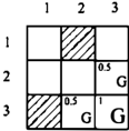
A robot is located somewhere in a room. The point is to define a policy that is able to bring it into the down-right square of the room shown in Figure 1. The objective will be partially satisfied if the robot ends in one of the neighbor squares. The state-space and the utility function tt on the objective states (taking its values in a finite subset of the interval (0, 1]) are depicted in Figure 1. tt(B33) = 1, p(s23) = p(s32) 0.5 and p(s) = 0 for the other states.

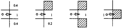
The available actions are to move (T)op, (D)own, (L)eft, ( R)ight or to (S)tay in place. If the robot chooses to stay, it will certainly remain in the same square. If it goes T, D, L or R it will (entirely) possi­ bly reach the desired square ( 1r = 1) if it is free but it will be possible that it reaches a neighbor square, as depicted in Figure 2 for the action R. The other tran­ sition possibility functions are of course symmetric to these.

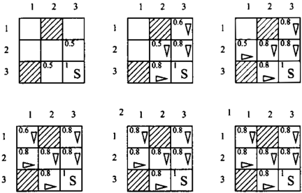
Let us now compute the optimal actions after one it­ eration of algorithm 4. For every action a and state s, we have Q 1 (s, a) = min,'esmax(1rr(s'ls, a), p(s')) ( rr does not depend on the stage) and u! ( s) = -1 maxae{T,D,L,R,s}Q (s, a).

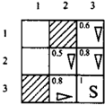
Figure 3 Resumes the utility of each state after one iteration, as well as an action that is optimal if the problem is assumed to be solved in one iteration only, for each state with a non-null pessimistic utility. The optimal action is uniq4e, except for state s33 for which D and R would be optimal actions as well.

Now we can iterate the process and get an optimal pol­ icy. The iterated process is described in Figure 4. Note that after 4 iterations, the utility of each state and the associated optimal action do not change anymore.

The number of iterations required to find a stationary policy is about the number of steps of the longest path from any state to goal state S, actions being assumed to be deterministic.

v v

4 POSSIBILISTIC PARTIALLY OBSERVABLE MULTISTAGE DECISION

4.1 BACKGROUND ON POSSIBILISTIC CONDITIONING

Conditioning has been defined in possibility theory (see [Dubois & Prade1994] for a complete presenta­ tion). As applied to events, possibilistic condition­ ing shall obey a form which is similar to the one of Bayesian conditioning :

where * can be min (see [Hisdal1978]) or product.

As the framework we choose to consider is purely or­ dinal, the only choice left is the operator min. Unlike in Bayesian conditioning, equation ( o: ) does not have a unique solution II(BIA). It is common then, after [Dubois & Prade1990], to choose the solution to ( o: ) which has the minimum specificity, thus leading to de­ fine II(BIA) as :

IT(BIA) = 1L ifii(AnB) = IT(A) >OL and II(BIA) = IT(A n B) otherwise.

Once the conditioning of possibility measures has been defined in this way, the conditioning of a possibility distribution by an observation o E 0 ( rr( ·lo)) can be defined as :

Definition 1 Conditional possibility distribution : rr(slo) = 1L if rr(s, o) = II(o) and rr(slo) = rr(s, o) otherwise. Where IT(o) = max,rr(s,o) and rr(·, · ) is a joint possibility distribution over S x 0.

4.2 POSSIBILISTIC POMDPs

We have already seen how classical POMDPs can be translated into MOPs over a belief state space. In a similar way, we are going to see how possibilis­ tic POMDPs (II-POMDPs) can be translated into IT­ MOPs over a possibilistic belief state space.

First of all, let us define a possibilistic belief state, f3 as a possibility distribution over the state space, ex­ pressing a plausibility ordering over the states. Unlike the set of probabilistic belief states, the set of possi­ bilistic beliefs is finite, as soon as we assume that the possibility degrees take their values in a finite set L (the cardinal of the possi bilistic belief state space B is bounded by lSI X ILl).

Suppose now that as in the probabilistic case, the transition possibilities rr(sls', a ) are given, as well as the observation possibilities rr(ols, a). Similarly to [Cassandra, Kaelbling, & Littman1994] we can define f3a(s) as the possibility of reaching state s, from an initial belief f3 and after the execution of action a :

We can also compute the possibility of observing o E 0 after having applied a in the (possibilistic) belief state [3 :

Now, [3� is the revised possibilistic belief state, after a was applied in f3 and o was observed :

• f3�(s) = OL if rr(ols, a ) = OL, f3�(s) rr(ols, a)= f3a(o)
• [3g ( s) = f3a ( s) in the other cases.

Then, all the elements of the new II-MOP over possi­ bilistic belief states are defined in equations (13), (14) and (15). The new II-MOP may be intuitively ex­ pressed as : from a state f3, applying action a may lead to one of the 101 states [3�, the possibility of reaching [3� being f3a(o) = rr(o l f3,a).

From now on, the "possibilistic" Bellman equation (pessimistic case) can be extended to the partially ob­ servable case :

where �J(f3) = min,es max{ n(f3(s)), �J(s)} and u�(/3) is initialized to �J(/3).

In the same way, the Q function becomes :

Algorithm 4 can now be extended to the partially ob­ servable case (in case no intermediate satisfaction de­ gree is involved).

一

Algorithm 5: Possibilistic value iteration in the par­ tially observable case

begin u. (,B) = J.l (,B), 'I f3 E B ; repeat for f3 E B do l for a E A do Q(,B, a ) +--mino§O max{ n (f3a( o )), u.(,B�)} ; u. (,B) +--maXa Q(f3, a ) ; until Q converges to Q*; return (J* end

Here, B is the set of belief states, which size is at most ILP51. For a given f3 and a given a, evaluat­ ing Q(,B, a ) needs 101 computations of (3�, which needs about lSI elementary computations (as {3� is immedi­ ately deduced from f3a ( o ) ) . The algorithm will perform at most IBI x ILl x IAI iterations before convergence. Finally, the overall complexity of the algorithm is in O(l£1 2 151+1 x IAI2 x JOI). This worst-case complexity is of course exponential in the size of the state space, in the general case, but it can be reduced when the sub­ set of belief states that can be reached from an initial belief state is small.

Example

Le us take again the preceding example, but assume now that observability is no more complete : all what the robot knows when it is in a given state (square) is the configuration of the walls around the square. Initially, the robot observes nothing, that is it can be anywhere in the state space depicted in figure 1.

Let us assume also that the observations are not noisy, then it can be shown that the belief states that can be reached from the initial belief state, applying any policy are limited to the following set of subsets of S : B = {S, {s21,s32} , {sn}, {s23} , {s32} , {s33} , { su, SJ3} , { s 2 I} } . These 8 belief states will be denoted by (30 to (3 7 . We can compute J.l(f3;) from the utility function over S : J.l(f3o) = J.l(f3J) = J.l(f32 ) = J.l(f3s) = J.l(f3 7 ) = 0, J.l(f33) = Jl(f34) = 0.5 and J.l(f35) = I .

The possibilities of transition from any belief state to any other, given an action a can be computed from the f3a ( o ) 's and the (3� 's, for o E 0. For example, if the initial belief state is (30 = S, and the action that is performed is (D)own, then the resulting belief states can be (3 1 , (33 or ,135 with possibility 1L, and f32 with possibility 0.2.

The utility function is modified after each iteration :

• Iteration 1 : u.(f35) = 1 = Q(f35, S) ; u.(f33) =

• Iteration 2 : u.(f32) = 0.8 = Q(f32, D) ; u.(,BI ) = 0.5 = Q(,B 1 , R) ; u.(f37 ) = 0.5 = Q(f37, R) ;
• Iteration 3 : u. (,BI) = 0.8 = Q(f3I , R) ; u. ((3 7 ) = 0.8 = Q(f37, R) ; u.(f3s) = 0.5 = Q(f3s, D) ; u.(f3o) = 0.5 = Q(f3o, D) ;
• Iteration 4: u.(,Bs) = 0.8 = Q(f3s, D) ; u.(f3o) = 0.5 = Q(f3o, D) ;

Iteration 5 does not change any value, so the algo­ ri thm has converged to the following optimal policy (which pessimistic utility is 0.8 whatever the initial state, except if the initial state is (35, where its util­ ity is 1) : (f3o, D), ({31, R), ((32, D), (f3a, D), ((34, R), ((35, S), (,Bs, D), ({37, R).

5 CONCLUSION

In this article we have proposed a qualitative coun­ terpart of POMDPs, based on possibility theory, and in particular on the use of the pessimistic possibilistic decision criterion advocated in [Dubois & Prade1995].

The possibilistic view of multistage decision under uncertainty permits a kind of decomposability of the sequential problem that allows to use dynamic programming-like algorithms for computing optimal policies. In particular, after we described the pos­ sibilistic backwards induction algorithm proposed in [Fargier, Lang, & Sabbadin1998] for the finite-horizon case, we proposed a modified version, similar to the value iteration algorithm, able to cope with problems in which the horizon is not fixed a priori.

In order to take partial observability into account in the possibilistic framework, we need to use condi­ tioning. Unfortunately, unlike in the stochastic case, there exists no universally accepted notion of condi­ tioning. We chose the one proposed by [Hisdal1978] as it fits well our qualitative (ordinal) framework and it is rather intuitive. Once a possibilistic notion of condi­ tioning is adopted, it is possible to see how belief states (i.e. possibility distributions) are updated after an ac­ tion is applied and an observation is made. Then, we were able to define the ll-POMDP framework and we showed how ll-POMDPs can be translated into fully observable ll-MDPs over an exponentially larger (but finite) state space.

The algorithm that we proposed for computing op­ timal policies in the possibilistic partially observable case is based on the possibilistic value iteration algo­ rithm used in the fully observable case. Another ap­ proach could be used in which a ll-POMDP is viewed

as a game against Nature : trying to maximize the value of the pessimistic criterion amounts to behave like in a game in which Nature chooses the "worst possible" observation, after an action is applied.

Finally, the compatibility of the possibilistic decision criterion with some structured representations of deci­ sion problems, particularly in the framework of possi­ bilistic logic should be pointed out. In (Sabbadin1998] it is shown that the possibilistic (pessimistic) one stage decision problem can be stated as an abduction prob­ lem with two stratified bases of formulas, one for mod­ eling uncertain knowledge and the other for model­ ing gradual preferences. Extending this framework to the multi stage, partially observable case, would allow to elaborate a structured language for ll-POMDPs as well as dedicated resolution algorithms.

References

• (Bellman1957] Bellman, R. E. 1957. Dynamic Pro­ gramming. Princeton University Press, Princeton.
• (Bertsekas & Tsitsiklis1989] Bertsekas, D. P., and Tsitsiklis, J. N. 1989. Parallel and Distributed Com­ putation: Numerical Methods. Englewood Cliffs: Prentice-Hall.
• (Bertsekas1987] Bertsekas, D. P. 1987. Dynamic Pro­ gramming: Deterministic and Stochastic Models. Englewood Cliffs: Prentice-Hall.
• (Brafman1997] Brafman, R. I. 1997. A heuristic variable grid solution method for pomdps. In Proc. of 13th Nat. Conf. on Artificial Intelligence (AAA/'97), 727-733.
• (Cassandra, Kaelbling, & Littman1994] Cassandra, A. R.; Kaelbling, L. P.; and Littman, M. L. 1994. Acting optimally in partially observable stochastic domains. In Proc. 11th Nat. Conf. on Ar­ tificial Intelligence ( AAA/'94), 1023-1028. Seattle, WA: AAAI Press.
• (Dubois & Prade1990] Dubois, D., and Prade, H. 1990. The logical view of conditionning and its ap­ plication to possibility and evidence theory. Int. J. of Approximate Reasoning 4(1):23-46.
• [Dubois & Prade1994] Dubois, D., and Prade, H. 1994. A survey of belief revision and updating rules in various uncertainty models. Int. Journal of Intel­ ligent Systems 9:61-100.
• (Dubois & Pradel995] Dubois, D., and Prade, H. 1995. Possibility theory as a basis for qualitative decision theory. In Proc. 14th Inter. Joint Conf. on Artificial Intelligence (IJCAI'95), 1925-1930.
• (Dubois, Prade, & Sabbadin1998] Dubois, D.; Prade, H.; and Sabbadin, R. 1998. Qualitative decision theory with sugeno integrals. In Cooper, G. F., and Moral, S., eds., Actes de la 14eme Conf. Uncertainty in Artificial Intelligence (UA/'98}, 121-128. Madi­ son, WI: Morgan Kaufmann.
• (Fargier, Lang, & Sabbadin1998] Fargier, H.; Lang, J.; and Sabbadin, R. 1998. Towards qualitative ap­ proaches to multi-stage decision making. Int. Jour­ nal of Approximate Reasoning 19:441-471.
• (Hauskrecht1997] Hauskrecht, M. 1997. Incremental methods for computing bounds in partially observ­ able markov decision processes. In 13th Nat. Conf. on Artificial Intelligence (AAAI'97), 734-739.
• (Hisdall978] Risdal, E. 1978. Conditional possibilities-independence and non-interactivity. Fuzzy Sets and Systems 1:283-297.
• (Lovejoy1991] Lovejoy, W. S. 1991. A survey of al­ gorithmic methods for partially observed markov decision processes. Annals of Operation Research 1(28):47-65.
• (Monahan1982] Monahan, G. E. 1982. A survey of partially observable markov decision processes. Management Science 1(28):1-16.
• (Parr & Russell995] Parr, R., and Russel, S. 1995. Approximating optimal policies for partially observ­ able stoc. In Int. Joint Conf. on Artificial Intelli­ gence (IJCA/'95), 1088-1094.
• (Puterman1987] Puterman, M. L. 1987. Encyclope­ dia of Physical Science and Technology. Academic Press. chapter Dynamic Programming, 438-463.
• (Puterman1994] Puterman, M. L. 1994. Markov De­ cision Processes. New York: John Wiley and Sons.
• (Sabbadin1998] Sabbadin, R. 1998. Decision as ab­ duction. In Proc. 13th European Conf. on Artificial Intelligence (ECAI'98}, 600-604.
• (Savage1954] Savage, L. J. 1954. The Foundations of Statistics. New York: J, Wiley and Sons.
• (von Neumann & Morgenstern1944] von Neumann, J., and Morgenstern, 0. 1944. Theory of Games and Economic Behavior. Princeton Uni­ versity Press.