A Transformational Characterization of Equivalent Bayesian Network Structures

David Maxwell Chickering Computer Science Department University of California at Los Angeles

dmax@cs. ucla. edu

Abstract

We present a simple characterization of equivalent Bayesian network structures based on local transformations. The sig­ nificance of the characterization is twofold. First, we are able to easily prove several new invariant properties of theoretical in­ terest for equivalent structures. Second, we use the characterization to derive an ef­ ficient algorithm that identifies all of the compelled edges in a structure. Compelled edge identification is of particular impor­ tance for learning Bayesian network struc­ tures from data because these edges indi­ cate causal relationships when certain as­ sumptions hold.

1 INTRODUCTION

A Bayesian network for a set of variables U = {x1, . . . , Xn} represents a joint probability distribu­ tion over those variables. It consists of (1) a network structure that encodes assertions of conditional inde­ pendence in the distribution and (2) a set of condi­ tional probability distributions corresponding to that structure. The network structure is an acyclic directed graph ( dag for short) such that each variable x; in U has a corresponding node x; in the structure.

For any given network structure, there is a correspond­ ing set of probability distributions that can be repre­ sented using a Bayesian network with that structure. Two network structures are equivalent if the set of dis­ tributions that can be represented using one of the dags is identical to the set of distributions that can be represented using the other. Because equivalence is re­ flexive, symmetric, and transitive, the relation defines a set of equivalence classes over network structures.

The notion of equivalence is of particular importance for learning Bayesian networks from data. As we will see in Section 4, compelled edges edges with in­ variant orientation for all structures in an equivalence class - can indicate causal relationships when certain assumptions hold.

There are two major contributions of this paper. First, we derive a characterization of equivalent network structures based on local transformations. This char­ acterization is presented here fully for the first time, although the result is used in earlier works by Hecker­ man et al. (1994) and Chickering et al. (1995). The characterization leads to a simple method for prov­ ing invariant properties over equivalent structures. We use the method to easily prove that Bayesian networks with equivalent structures require the same number of parameters, and that several well-known scoring met­ rics used for learning Bayesian network structures from data give the same score to equivalent structures. In addition, we easily prove a graph-theoretic property of equivalent structures that is used by Chickering et al. (1995) to derive an important complexity result.

The second contribution of this paper is the presen­ tation of an efficient algorithm to identify all of the compelled edges in a given network structure. We use the transformational characterization to prove the cor­ rectness of the algorithm, and present an implementa­ tion of this algorithm that is asymptotically optimal on average.

In Section 2 we describe our notation and introduce previous relevant work. In Section 3 we derive the characterization and prove some invariant properties for equivalent structures. In Section 4 we present a compelled edge identification algorithm and analyze the complexity for various implementations.

2 NOTATION

In this section we introduce our notation and discuss previous relevant work on which our characterization is based.

A Bayesian network B is a pair ( g, Og) where g = (U, Eg) is a dag, and Og is the set of conditional prob­ ability distributions that correspond tog. Throughout this paper, we make many comparisons between dags. It is to be assumed that whenever we make such a comparison, the dags in question are all defined over

the same set of vertices U, and that the only difference is the set of edges connecting these vertices.

Although we already defined equivalence in Section 1, we present a more formal definition here.

Definition 1 Two dags g and g' are equivalent if for every Bayesian network B = ( g, Og), there exists a Bayesian network B' = (Q', Og·) such that B and B' define the same probability distribution, and vice versa.

We use g � g' to denote that g and g' are equivalent. As was stated earlier, the relation � defines a set of equivalence classes over the network structures. We often say that two Bayesian networks are equivalent when we mean that the structures of those networks are equivalent.

A directed edge Xi ___. Xj E Eg is compelled in g if for every dag g' � g, Xi __. Xj E Eg·. For any edge e E Eg, if e is not compelled in g, then e is reversible in g, that is, there exists some dag g' equivalent to g in which e has opposite orientation. We use Cg and Rg to represent the set of compelled and reversible edges in g respectively. For any node Xi in some dag g, we use rrr to denote the set of parents of Xi in g. When the dag g is clear from context, we use II; instead. For notational simplicity, we often use symbols without indices for nodes in a dag. In this case, we subscript II with the full name of the node. For example, we use IIy to denote the parent set of node y.

The notion of a covered edge is very important in the sections to follow, so we emphasize the definition here.

Definition 2 An edge e = x ___. y E Eg is covered in g if II�= II� U x.

I n other words, x ___. y is covered in g if x and y have identical parents in g, with the exception that x is not a parent of itself.

The skeleton of any dag is the undirected graph result­ ing from ignoring the directionality of every edge. For any pair of dags g and g' that share the same skeleton, we use A.( g, g') to denote the set of edges in g that have opposite orientation in g'. A v-structure in dag g is an ordered triple of nodes (x, y, z ) such that (1) g contains the arcs x ___. y and z ___. y, and (2) x and z are not adjacent in g.

The characterization of equivalent structures that we present in the next section is based on that derived by Verma and Pearl (1990) which reads:

Theorem 1 {Verma and Pearl, 1990} Two dags are equivalent if and only if they have the same skeletons and the same v-structures.

A consequence of Theorem 1 is that for any edge e participating in a v-structure in some dag g, if that edge is reversed in some other dag g', then g and g' are not equivalent.

A topological sort of the nodes in a dag g is any total ordering of the nodes such that for any pair of nodes x; and x j in g, if x; is an ancestor of xi, then Xi must precede Xj in the ordering.

3 THE CHARACTERIZATION AND SOME CONSEQUENCES

In this section we derive a simple local characteriza­ tion of equivalent network structures. Simply stated, we show that a property holds for all pairs of equivalent networks that differ by a single covered edge orienta­ tion if and only if that property holds for all networks in the equivalence class. In Sections 3.1 to 3.3, we use this new characterization to prove several invari­ ant properties of equivalent structures.

While preparing the final version of this work, we be­ came aware of two previous attempts to prove the cor­ rectness of the characterization. Madigan (1993) uses the characterization to prove a property of equivalent structures similar to that of Theorem 1. Bouckaert (1993a) uses the characterization to prove a property of the MDL scoring metric that we explore in Sec­ tion 3.2. The proof we provide in this section, unlike previous ones, includes the necessary step of demon­ strating the existence of an edge that can be reversed and, moreover, explicates constructively how such an edge is found.

As we see in Lemma 1, for any pair of dags that differ by a single edge reversal, there are simple, local, nec­ essary and sufficient conditions for determining if the dags are equivalent.

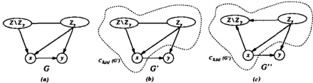
Lemma 1 Let g be any dag containing the edge x ___. y, and let g' be the directed graph identical to g except that the edge between x and y in g' is oriented as y ___. x. Then g' is a dag that is equivalent tog if and only if x ___. y is a covered edge in g.

Proof:

(if) Assume that x ___. y is a covered edge in g. That is, II� = II� U x. First we show that g' is a dag. If g' contained a cycle, then this cycle must include the edge y ___. x because g is a dag. Thus there must be a directed path from x to y in g which does not include the edge x ___. y. Let z be the last node in this path. By assumption, z is a parent of both x and y in g, and because there is a directed path from x to z, this implies that g contains a cycle, which contradicts the fact that g is a dag.

Now we show that g' � g. Because g and g' have the same skeletons, if g' ¢ g then one of the dags must contain a v-structure that is not in the other dag. Suppose that g' contains-a v-structure not in g. This v-structure must include the edge y ___. x because this is the only edge that differs between g' and g. But this implies that x has a parent that is not adjacent to y in both graphs, contradicting the assumption that every

parent of x is also a parent of y in g. If we assume that g contains a v-structure not in 9', a similar argument also yields a contradiction.

(only if) We now show that if x -+ y is not a covered edge in g, then either g' contains a directed cycle, or g' is a dag that is not equivalent to g. If x-+ y is not a covered edge in g, at least one of the following two conditions must hold in g: (1) Some node z -:f x is a parent of y but not a parent of x. (2) Some node w is a parent of x but not a parent of y.

Let z -:f x be a parent of y in g which is not a parent of x in g. If z and x are not adjacent, then (x, y, z ) is a v-structure in g that does not exist in g'. If x is a parent of z in g, then by definition of g', it follows that x is a parent of z in g' and therefore g' contains a directed cycle.

Let w be a parent of x in g which is not a parent of y in g. If w and y are not adjacent, then ( w, x, y) is a v-structure in g' that does not exist in g. The node y cannot be a parent of w in g, lest g would contain a directed cycle. 0

Smith (1989) proves the (if) part of Lemma 1 using an additional precondition.

Clearly any property that holds over all dags in an equivalence class must hold over every pair of dags in that class which differ by the orientation of a single covered edge. We prove the converse by showing that for any pair of equivalent dags g and g', we can trans­ form g into g' by a series of covered edge reversals, where each reversed edge is from .6.(9, g'). As we see below, identifying a covered edge in .6.(9, g') is simple.

Algorithm Find-Edge(9, g')

Input: Equivalent dags g and g' that differ by at least one edge

Output:

Edge from .6.(9, g')

(Let Pv = {ulu-+ v E .6.(9,g')}.)

1. Perform a topological sort on the nodes in g
2. Let y be the minimal node with respect to the sort for which Py -:f 0
3. Output x -+ y
4. Let x be the maximal node with respect to the sort for which x E Py

Lemma 2 The edge x -+ y output from Algorithm Find-Edge(9, g') is a covered edge.

Proof: Suppose that x -+ y is not a covered edge. Let z -:f x be any parent of y that is not a parent of x. If z is not adjacent to x then x -+ y participates in a v­ structure in g that cannot be in g', contradicting the fact that g � g'. If x -+ z is in g, then either this edge or z -+ y must be in .6.(g, g'), lest g' would contain a directed cycle. If x -+ z is in .6.(g, g') then z would have been chosen instead of y in Step 2. If z -+ y is in .6.(9, g'), then z would have been chosen instead of x in Step 3. If we assume that there exists a parent of x that is not a parent of y, a similar argument yields a contradiction. 0

Using Lemmas 1 and 2 we can prove the characteriza­ tion.

Theorem 2 Let g and g' be any pair of dags such that g � g'. There exists a sequence of 1 .6.(9, g')l dis­ tinct edge reversals in g with the following properties:

1. Each edge reversed in g is a covered edge
2. After each reversal, g is a dag and g � 9'
3. After all reversals, g = g'

Proof: We show that all the conditions hold if we use Procedure Find-Edge with input g and 9' to identify the next edge x -+ y to reverse. By Lemma 2, x -+ y is a covered edge and Condition 1 holds. By Lemma 1 and Condition 1, Condition 2 holds. Af­ ter each reversal 1.6.(9, g')l decreases by one and thus Condition 3 holds. 0

Using Theorem 2, we can prove that a given property is invariant over all equivalent structures simply by showing that the property is invariant to any rever­ sal of a single covered edge. In the sections to follow, we prove that several theoretically interesting proper­ ties are invariant over equivalent structures using this technique.

3.1 NUMBER OF PARAMETERS

In this section, we use Theorem 2 to prove that Bayesian networks with equivalent structures require the same number of parameters.

Consider a Bayesian network B = (g, Og) where g = (U, Eg). For any node Xi C U, we use r; to be the number of states of x;. For each node Xi with parents II;, Og contains the conditional probability distribu­ tion p(x;III;). We use Dim(x;,II;) to represent the number of logically independent parameters needed to represent p(x;III;). For every distinct parent instan­ tiation, there are r; -1 independent parameters, and therefore

We use Dim(9) to represent the number of parame­ ters needed to completely specify Og. We can express Dim(9) as follows:

Theorem 3 If g � g' then Dim(9) = Dim(9').

Proof: From Theorem 2, we need only show that the theorem holds when g and g' differ by the orientation of a single covered edge. Let x; -+ Xj be this edge in g.

For any node Xk, let lh and II� be the parents of node Xk in 9 and 9' respectively. Because every node except for x; and xi have identical parents in 9 and 9', we need only show that

Dim(x;, II;) + Dim(xj, Ilj) = Dim(x;, IID + Dim(xj, IIj)

Plugging Equation 1 into the above expression we have

By definition of a covered edge, Ilj = II; U x;. Fur­ thermore, because x; ---+ Xj is the only edge that dif­ fers between 9 and 9'' we have rr: = II; u X j and Ilj = II;. After plugging these equalities into Equa­ tion 2 and dividing both sides of the resulting equation by Ti xkE II ; rk, it is easy to see that the equality holds. 0

It follows from Theorem 1 and Theorem 3 that the space needed to represent an arbitrary distribution is identical for all equivalent Bayesian networks. Other consequences of Theorem 3 will be explored in the fol­ lowing section.

3.2 SCORE EQUIVALENCE

In this section, we use Theorem 2 to prove that several scoring metrics for learning Bayesian networks from data give the same score to equivalent structures.

A scoring metric is a function that takes as input a Bayesian network structure, a database of observed cases, and possibly some prior knowledge, and returns a value reflecting how well the structure fits the data. We use C = { Ct, . . . , CN } to represent the database of N observed cases and { to represent our prior knowl­ edge. We assume that for each case C;, every variable in U is observed. 1

A metric M is score equivalent if and only if

for all choices of C and {. When a metric does not use prior information, we omit the argument e.

For a structure 9, we define the likelihood L of the observed data as a function of 9, C and the parameters Bg as follows:

where 9h is the hypothesis that the data was generated by a distribution that can be factored according to 9.2

1 Researchers typically make this assumption for com­ putational efficiency. Methods exist for scoring structures when there is missing data.

2This is an acausal interpretation of a network struc­ ture. Heckerman et al. (1994, 1995) investigate a causal interpretation of a network structure as well.

It follows by the definition of 9h that the hypotheses corresponding to equivalent structures are identical. We call this property hypothesis equivalence.

The maximum likelihood metric of a structure 9 is de­ fined as

It follows almost immediately from the definition of equivalent structures that the maximum likelihood metric is score equivalent. Maximum likelihood is not very useful as a scoring metric by itself because any complete network structure will always get the high­ est possible score. Many of the metrics we are about to discuss, however, are defined as the sum of MML and a penalty term.

The first scoring metric we consider, introduced by Akaike (1974), is called the A information criterion ( AIC ) . In the context of scoring Bayesian networks, MAIC can be expressed as follows:

Theorem 4 MAIC is score equivalent.

Proof: Follows immediately from Theorem 3 and the fact that MM L is score equivalent. 0

Another scoring metric introduced by Schwarz (1978) is the Bayesian information criterion ( BIC ) . This met­ ric is defined as

where N is the number of cases in C.

Theorem 5 MniC is score equivalent.

The proof of Theorem 5 is identical to the proof of Theorem 4.

Rissanen (1986) presents two scoring metrics using the principle of minimum description length ( MDL ) . One of these metrics, originally presented in Rissanen (1978), has recently received some attention in the lit­ erature. A version of this metric explored by Bouck­ aert (1993b) is

where p(9h) is the prior probability of hypothesis 9h, and H((i, C) is the entropy of the distribution resulting from parameterizing 9 with the appropriate fractions in the data. It can be shown that -N · H (9, C) is identical to the log of the maximum likelihood metric. Therefore equation 4 reduces to

Theorem 6 MMDLl is score equivalent.

Proof: Follows immediately from hypothesis equiva­ lence and Theorem 5. 0

Theorem 6 was also proven by Bouckaert (1993a). An­ other version of the MDL metric presented by Lam and Bacchus (1993) can be written as

where c is a constant that represents the number of bits needed to store a numerical value to some specified precision. We can again eliminate the entropy term to obtain

Theorem 7 MMDL2 is score equivalent.

Proof: The first term is score equivalent by defini­ tion of equivalent structures. The second term is score equivalent by Theorem 1. The third term is score equivalent by Theorem 3. 0

The last metric we consider is a Bayesian metric dis­ cussed by Beckerman et al. (1994, 1995) known as the BDe metric. A Bayesian metric is any metric that ex­ presses the relative posterior probability of the struc­ ture hypothesis, given the observed cases and prior knowledge. Specifically, for any Bayesian metric M we have

The first term in Equation 5 is the prior probability of the structure hypothesis. The second term, which we call the likelihood of the data, is the posterior proba­ bility of the data given the structure hypothesis. The third term is an arbitrary constant.

Beckerman et al. (1994, 1995) derive a closed form expression for the likelihood term of Equation 5 using some assumptions about prior densities over Og. Be­ fore we present the expression, we need the following notation. qi is the number of distinct instantiations of the parents of node Xi. Nij k is the number of cases in 6 for which x; = k and II; in its jth configuration.

where Nfik = p(x; = k,II ; = ile ), N;j = Lk Niik and Nfj = Lk Nfjk " r is the Gamma function, which satisfies r(x + 1) = xr(x). In practice, researchers can use a prior network to determine both p(x; = k, II; = ile) and a reasonable prior distribution p(Q h le ).

The BDe metric is defined to be the Bayesian metric of Equation 5 for which the likelihood term is computed using Equation 6. We say that a Bayesian metric is likelihood equivalent if p ( Clg h , e ) is score equivalent. Beckerman et al. (1994, 1995) use Theorem 2 to prove the following result.

Theorem 8 MsDe is likelihood equivalent.

It follows by hypothesis equivalence that MsDe is score equivalent as well. 3

3.3 NUMBER OF PARENTS

In this section we present yet another consequence of Theorem 2. This result was used by Chickering et al. (1995) to prove that the Bayesian approach to learning Bayesian networks from data is NP-hard.

Theorem 9 Let g and 9' be any pair of dags such that g ::::: 9'. If g has a node with exactly k parents, then 9' has a node with exactly k parents.

Proof: From Theorem 2, we need only show that the theorem holds when g and 9' differ by the orientation of a single covered edge. Let x -+ y be this edge in g.

Because every node except for x and y have identical parents in g and 9', the theorem holds trivially unless the only node in g that has k parents is either x or y. From the definition of a covered edge it follows that in 9', x has the same number of parents that y has in g and y has the same number of parents that x has in g. 0

4 IDENTIFYING COMPELLED EDGES

In this section we first discuss the significance of com­ pelled edge identification for learning networks from data and explore previous relevant work. Next we present an algorithm that identifies the set of all com­ pelled edges in an equivalence class. Finally, we discuss an implementation of the algorithm that is asymptot­ ically optimal on average.

As was mentioned in Section 1, identifying compelled edges is of particular importance for learning Bayesian networks from data because these edges can indicate causal influences. The assumptions needed to infer causation from the compelled edges are ( 1) if two vari­ ables are statistically dependent in every observable context, then one of the variables is a direct cause of the other, and ( 2) if two variables are statistically inde­ pendent in some (possibly empty) observable context, then neither variable is a direct cause of the other. Note that the first assumption excludes the possibility that there is a hidden common cause of two variables. Spirtes et al. (1993) call Assumption 1 causal suffi­ ciency and Assumption 2 faithfulness. Assumption 2 is called stability by Pearl and Verma (1991) . If an equivalence class is learned with certainty and the as­ sumptions hold, then all the compelled edges denote causal influences.

3Theorem 8 was proven without the assumption of hy­ pothesis equivalence. It follows that the result also applies to causal interpretations of structures for which hypothesis equivalence does not hold.

There are two distinct approaches that researchers use to learn Bayesian networks from data. The first ap­ proach, which we call the metric approach, uses a scor­ ing metric to measure how well a particular structure fits an observed set of cases. A search algorithm is typically used to identify one or more structures that attain a high metric score. As we saw in Section 3.2, many of the metrics that researchers use have the prop­ erty of score equivalence. It follows that when using a score equivalent metric, the metric approach to learn­ ing is in fact a method for identifying entire equiva­ lence classes. We assume in this section that a score equivalent metric is being used in the metric approach.

In the second approach to learning, which we call the independence approach, an independence oracle is queried to identify the equivalence class that captures the independencies in the distribution from which the observed data was generated.

One distinction between the two learning approaches is the way equivalence classes are represented. Using the metric approach, an equivalence class is represented by any element in the class. We call this the canonical element representation scheme. In the independence approach, researchers typically use an acyclic partially directed graph ( pdag for short ) to represent the equiv­ alence class.

From Theorem 1, the only edges that need be directed in a pdag representation to uniquely identify an equiv­ alence class are those that participate in v-structures. If, in fact, these are the only directed edges in the pdag, we say that the graph is a minimal pdag representation of the equivalence class. If a pdag has the property that every directed edge corresponds to a compelled edge, and every undirected edge corresponds to a re­ versible edge for every dag in the equivalence class, then we say it is a completed pdag representation.

When using the independence approach to learning, researchers use a statistical test ( such as chi-square ) to approximate the independence oracle, and the learn­ ing algorithm builds a unique minimal pdag represen­ tation of the equivalence class. We refer the reader to Verma and Pearl (1992) or Spirtes et al. (1993) for the details of this procedure.

Previous work on compelled edge identification can be understood in the context of the independence ap­ proach to learning. After identifying a minimal pdag representation of an equivalence class, the learning al­ gorithm searches for the remaining compelled edges that do not participate in v-structures by matching patterns of directed and undirected edges. When a match is found, one or more undirected edges in the pdag are directed and the process continues. Verma and Pearl (1992) present an algorithm of this type that is known to be sound, but not complete. That is, every directed edge in the final pdag is provably compelled, but not every undirected edge is provably reversible. More recently, both Meek (1995) and Anderson et al. (1995) have derived sound and complete algorithms for constructing a completed pdag representation.

The algorithm we present in this section takes a dag as input, and labels every edge in the dag as either com­ pelled or reversible. We show that the algorithm is correct and discuss an implementation that is asymp­ totically optimal in the average case. Our algorithm is also applicable to identifying compelled edges when the equivalence class is represented with a pdag. Dor and Tarsi (1992) present a polynomial-time algorithm that takes as input a ( possibly minimal ) pdag repre­ sentation of an equivalence class, and returns a canon­ ical element representation. Unfortunately, the algo­ rithm has a worst-case time complexity that is worse than that of of our identification algorithm. Nonethe­ less, if the equivalence class is represented as a minimal pdag, we get a significant improvement in asymptotic behavior over the previous algorithms by changing rep­ resentations and using our algorithm.

When the independence approach to learning is used, an equivalence class is determined with certainty. Be­ cause the data is finite, however, we have uncertainty about the learned equivalence class as a result of the approximation of the independence oracle. One ad­ vantage to using a Bayesian scoring metric instead of other metrics or the independence approach is that the uncertainty about any equivalence class is explicitly represented in the score of that class. Consequently, we can express our belief in the statement s = "x is a direct cause of y" by summing over all ( non-equivalent ) structures:

In practice, it is impossible to sum over all possible equivalence classes. Therefore we attempt to find a small subset of structure hypotheses that account for a large fraction of the posterior probability of the hy­ potheses. Chickering (1995) suggests a set of search operators that can be used to efficiently search for such a subset.

For those hypotheses in which x -+ y is compelled, the corresponding probability p( sJQh, �) term will be unity. If y -+ x is compelled or if x and y are not adjacent, then the term will be zero. If the edge between x and y is reversible, then p( sJQh, �) can take any value from zero to one and must be assessed directly.

Beckerman et al. (1994, 1995) discuss a causal inter­ pretation for the hypothesis g h . The hypothesis not only asserts that the distribution that generated C can be factored according to g, but that each node in the graph is a direct cause of its children. Using this in­ terpretation, the term p( sJQh, �) is either one or zero, depending on whether x -+ y is in g or not. When structures are interpreted causally, we no longer have the property of hypothesis equivalence. Nonetheless, we can sometimes still use entire equivalence classes to

calculate Equation 7. For example, if the prior prob­ ability distribution over structure hypotheses is uni­ form, then a likelihood equivalent learning metric is score equivalent. In this case, we can still take the sum in Equation 7 over non-equivalent structures and weight each term by the number of dags in the equiv­ alence class that contain the edge x --+ y. We are currently investigating techniques for efficiently deter­ mining such a weighting term.

In Section 4.1 we present the algorithm and prove that it correctly classifies all of the edges in a dag. In Sec­ tion 4.2 we discuss asymptotic running time behavior of various implementations.

4.1 THE ALGORITHM

The first step of the algorithm is to define a total or­ dering over the edges in the given dag. For simplicity, we present this step as a separate procedure listed be­ low. To avoid confusion between ordered nodes and ordered edges, we have capitalized "node" and "edge" below.

Algorithm Order-Edges(Q)

Input:

dag g

Output:

dag g with labelled total order on edges

1. Perform a topological sort on the NODES in g
2. Set i = 0
3. While there are unordered EDGES in g
4. Let y be the lowest ordered NODE that has an unordered EDGE incident into it
5. Let x be the highest ordered NODE for which x --+ y is not ordered
6. Label x--+ y with order i
7. i=i+ 1

The algorithm to find the compelled edges is as follows.

Algorithm Find-Compelled(Q)

Input:

dag g

Output:

dag g with each edge labelled either "com­ pelled" or "reversible"

1. Order the edges in g using Algorithm Order-Edges
2. Label every edge in g as "unknown"
3. While there are edges labelled "unknown" in g
4. Let x --+ y be the lowest ordered edge that is labelled "unknown"
5. For every edge w--+ x labelled "compelled"
6. If w is not a parent of y, then label x --+ y and every edge incident into y with "com­ pelled" and goto 3
7. Else label w--+ y with "compelled"
8. If there exists an edge z --+ y such that z =f x and z is not a parent of x, then label x --+ y and all "unknown" edges incident into y with "compelled"
9. Else label x --+ y and all "unknown" edges incident into y with "reversible"

Before proving the correctness of the algorithm, we need a few intermediate results. The proofs of the first two results, which are given in the Appendix, make extensive use of Theorem 2.

Lemma 3 Let g be any dag and let x, y and z be any three nodes that are all adjacent in g. If any two of the connecting edges are reversible, then the third one is also.

Lemma 4 Let g be any dag, and let x --+ y be any edge in g such that ITy � IIx U x. The edge x --+ y is reversible if and only if for every edge w --+ x such that w and y are not adjacent, w --+ x is reversible.

In addition to the above two lemmas, we find the fol­ lowing three simple results useful for proving the cor­ rectness of our algorithm.

Lemma 5 When x --+ y is chosen in Step 4 of the algorithm, every edge incident into node y is labelled "unknown".

Proof: Follows by noting that after any iteration of the while loop, every edge incident into y gets labelled with either "reversible" or "compelled". 0

Lemma 6 Let x --+ y be the edge chosen in Step 4 of the algorithm. Any parent of y that is ad jacent to x is a parent of x.

Proof: Let z be any parent of y that is adjacent to x. By Lemma 5 we know z --+ y i s labelled "unknown" . If x --+ z, then z --+ y has a lower order than x --+ y (see Algorithm Order-Edges) and would have been chosen in Step 4. 0

Lemma 7 Let x --+ y be the edge chosen in Step 4 of the algorithm. If x --+ y is compelled, then every edge incident into y is compelled.

Proof: Let z --+ y be any edge incident into y. If z and x are not adjacent, then z --+ y must be compelled because it participates in a v-structure. If z and x are adjacent, then from Lemma 6 we know the edge is oriented as z --+ x. If z --+ x is compelled, then there is a directed path from z to y in every graph equivalent to g and hence reversing z --+ y will always create a cycle. If z --+ x is in Rg , then by Lemma 3 z --+ y is compelled. 0

Now we prove the correctness of our algorithm.

Theorem 10 The edge labels resulting from the algo­ rithm are correct.

Proof: We prove that the labellings are correct by in­ duction on the number of iterations through the while loop.

When the first iteration of the while loop begins, all edges are labelled "unknown" . Thus for the edge x -+ y chosen in Step 4, there can be no edge w -+ x tested for in Step 5, lest this would be the first edge instead of x -+ y. Therefore IIx = 0 and the algorithm drops immediately to Step 8. There can be no edge z -+ y such that z and x are adjacent because by Lemma 6, we know that any edge between z and x is oriented as z -+ x which implies that x -+ y would not have been the first edge chosen. Therefore if any edge z -+ y is incident into y, that edge is part of a v-structure with x -+ y and therefore both z -+ y and x -+ y are compelled. Furthermore, by Lemma 7, all edges incident into y are compelled, so all labelling done in Step 8 is correct. If Step 9 is reached, no edge z -+ y exists and it follows that IIy = x. Because IIx = 0, x -+ y is reversible by Lemma 4, and the labelling done at Step 9 is correct.

Assume all labelling is correct for the first k -1 iter­ ations through the while loop of Step 3. Consider the edge x -+ y chosen in Step 4 on the kth iteration of the while loop.

From Step 6, if there is a compelled edge w-+ x such that w is not a parent of y then w and y are not ad­ jacent, lest (} contains a directed cycle. It follows that x -+ y must be compelled, lest there would exist a dag in the same equivalence class as (} with the extra v-structure ( w, x, y). By Lemma 7, it follows that all edges incident into y are compelled and therefore all labelling done in Step 6 is correct. If there is a com­ pelled edge w -+ x such that w and y are adjacent, then the edge between w and y must be oriented as w -+ y lest (} would contain a directed cycle. Further­ more, we deduce that this edge is compelled by the following argument: if x -+ y is compelled, then there is a directed path from w to y in every dag equivalent to (} and hence reversing w -+ y will always create a cycle; if x -+ y is reversible, then w -+ y is com­ pelled by Lemma 3. Thus all labelling done in Step 7 is correct.

From Step 8, if there exists a parent z of y that is not a parent of x, then by Lemma 6, z is not adjacent to x which implies x -+ y participates in a v-structure and is therefore compelled. Furthermore, by Lemma 7, all edges incident into y are compelled and hence all labelling done in Step 8 is correct.

If Step 9 is reached, every parent of y (with the ex­ ception of x ) is a parent of x. That is, IIy � IIx U x. Furthermore, because Step 9 is reached only if Step 6 always fails, every edge w -+ x for which w and y are not adjacent must be reversible. Consequently, we conclude from Lemma 4 that x -+ y is reversible.

Now consider any edge z -+ y incident into y that is labelled with "unknown". It must be the case that z -+ x is reversible, lest z -+ y would have been labelled "compelled" in Step 7. Thus we conclude from Lemma 3 that z -+ y is reversible and hence all labelling done in Step 9 is correct. D

4.2 COMPLEXITY ANALYSIS

In this section we investigate the asymptotic time behavior of various implementations of Algorithm Find-Compelled presented in Section 4.1. Because the algorithm labels every edge in the dag g, the best that any implementation can do is O(IEgl).

We first investigate an implementation of Algorithm Order-Edges that runs in time O(IEgl). We assume that(} is represented using the adjacency-list represen­ tation. It is well known that a topological sort can be performed in time O(IEg I) using a depth-first search. Once the nodes in the dag have been ordered, we would like to sort the parents of each node in descending or­ der. Once we have accomplished this, sorting the edges becomes trivial: step through each node in ascending sort order, and for each node, list all the incident edges by stepping through the sorted parent list.

One simple way to sort the parent pointers is as fol­ lows. Extend the representation to include child­ pointers for each node. This will take time O(IEg 1). Now step through each node in ascending order, and for each child of the current node, insert the current node at the front of the parent list. When the algo­ rithm completes (in time O(IEg I)) the parent pointers will be sorted in descending order.

From the above discussion, we see that Step 1 of Al­ gorithm Find-Compelled can be completed in time O(IEgl). Assume that with each node, we store sepa­ rate lists of "compelled", "reversible", and "unknown" incident edges (i.e. parents), so that these can be effi­ ciently accessed in the algorithm. We now consider the inside of the while loop. For each edge that we consider in Step 5, we necessarily label at least one "unknown" edge in either Step 6 or Step 7. Thus neither Step 5, Step 6 nor Step 7 can ever be executed more than lEg I times. Furthermore, for every edge considered in Step 8, that edge is "unknown" (See Lemma 7) and will get labelled in the current iteration of the while loop. Thus every operation within the while loop is executed no more than lEg I times.

We note that it is possible to get an amortized con­ stant time adjacency test in Step 6, but do not want to worry the reader with the details. Unfortunately, this is not the case for the adjacency test in Step 8. Because all labellings can be done in constant time, it follows that the time complexity of the entire algo­ rithm is dominated by the O(IEgl) executions of Step <8. If we use a hash table to store the parents of each node, we can complete the adjacency test in constant time on average. The resulting implementation of the algorithm will take time O(IEg I) on average, which is asymptotically optimal.

A problem with the hash table implementation is that in the worst case, each adjacency test can take O(IUI), resulting in a worst case O(IUI·IEgl) algorithm. If in­ stead we test for adjacency by performing a binary search over the parents of a node, each test can be

completed in time O(log lUI), and the resulting algo­ rithm takes time O(IEgl logiUI) in the worst case.

Ifg is represented with an adjacency matrix, then test­ ing for adjacency will always be a constant time op­ eration, and therefore Algorithm Find-Compelled takes time O(IE91) in the worst case. Building the ad­ jacency matrix, however, takes time O(IUI2) and will therefore dominate the time to complete the algorithm. For dense graphs, the use of an a,.djacency matrix is a good solution.

If an equivalence class is represented using a mini­ mal pdag, we can construct a completed pdag using a combination of our algorithm and the algorithm pre­ sented by Dor and Tarsi (1992) which returns a canon­ ical element given a minimal pdag. First we obtain the canonical element, which has been shown to take time O(IUI · IEgl). Next we run Algorithm Find­ Compelled to determine all the compelled edges. Fi­ nally we direct every undirected edge in the original pdag that corresponds to a compelled edge. The run­ ning time of the combined algorithm is dominated by the time to retrieve the canonical element and is there­ fore O(IUI·IEgl).

Acknowledgments

I would like to thank David Galles, Dan Geiger, Rich Korf, David Madigan, Chris Meek, Judea Pearl, and anonymous reviewers for useful suggestions. I owe spe­ cial thanks to David Beckerman, whose help and en­ couragement made this work possible. This work was supported by NSF Grant No. IRI-9119825, and a grant from Rockwell International.

References

[Akaike, 1974] Akaike, H. (1974). A new look at the statistical model identification. IEEE Transactions on Automatic Control, 19(6):716-723.

[Anderson et al., 1995] Anderson, S. A., Madigan, D., and Perlman, M. D. (1995). A characterization of markov equivalence classes for acyclic digraphs. Technical Report 287, University of Washington, Department of Statistics.

• [Bouckaert, 1993a] Bouckaert, R. (1993a). Belief net­ work construction using the minimum description length principle. Technical Report UU-CS-1994-27, Department of Computer Science, Utrecht Univer­ sity, The Netherlands.
• [Bouckaert, 1993b] Bouckaert, R. (1993b ). Probabilis­ tic network construction using the minimum de­ scription length principle. In ECSQARU, pages 4148.
• [Chickering et al., 1995] Chickering, D., Geiger, D., and Beckerman, D. (1995). Learning Bayesian net­ works: Search methods and experimental results. In
• Proceedings of the Fifth International Workshop on Artificial Intelligence and Statistics.
• [Chickering, 1995] Chickering, D. M. (1995). Search operators for learning equivalence classes of Bayesian network structures. Technical Report R231, Cognitive Systems Laboratory, UCLA Com­ puter Science Department.
• [Dor and Tarsi, 1992] Dor, D. and Tarsi, M. (1992). A simple algorithm to construct a consistent exten­ sion of a partially oriented graph. Technical Report R-185, Cognitive Systems Laboratory, UCLA Com­ puter Science Department.
• [Beckerman et al., 1994] Beckerman, D., Geiger, D., and Chickering, D. (1994). Learning Bayesian net­ works: The combination of knowledge and statis­ tical data. Technical Report MSR-TR-94-09, Mi­ crosoft.
• [Beckerman et al., 1995] Beckerman, D., Geiger, D., and Chickering, D. (1995). Learning discrete Bayesian networks. Machine Learning. to appear.

[Lam and Bacchus, 1993] Lam, W. and Bacchus, F. (1993). Using causal information and local mea­ sures to learn Bayesian networks. In Proceedings of Ninth Conference on Uncertainty in Artificial Intel­ ligence, Washington, DC, pages 243-250. Morgan Kaufmann.

• [Madigan, 1993] Madigan, D. (1993). A note on equivalence classes of directed acyclic independence graphs. Probability in the Engineering and Informa­ tional Sciences, 7(3):409-412.

[Meek, 1995] Meek, C. (1995). Causal inference and causal explanation with background knowledge. In Proceedings of Eleventh Conference on Uncertainty in Artificial Intelligence, To Appear. Morgan Kauf­ man.

• [Pearl and Verma, 1991] Pearl, J. and Verma, T. (1991). A theory of inferred causation. In Allen, J., Fikes, R., and Sandewall, E., editors, Knowl­ edge Representation and Reasoning: Proceedings of the Second International Conference, pages 441452. Morgan Kaufmann, New York.
• [Rissanen, 1978] Rissanen, J. (1978). Modeling by shortest data description. Automatica, 14(1):465471.
• [Rissanen, 1986] Rissanen, J. (1986). Stochastic com­ plexity and modeling. The Annals of Statistics, 14(3):1080-1100.
• [Schwarz, 1978] Schwarz, G. (1978). Estimating the dimension of a model. Annals of Statistics, 6:461464.
• [Smith, 1989] Smith, J. Q. (1989). Influence dia­ grams for statistical modelling. Annals of Statistics, 17(2):654-672.
• [Spirtes et al., 1993] Spirtes, P., Glymour, C., and Scheines, R. (1993). Causation, Prediction, and Search. Springer-Verlag, New York.

[Verma and Pearl, 1990] Verma, T. and Pearl, J. (1990). Equivalence and synthesis of causal models. In Proceedings of Sixth Conference on Uncertainty in Artificial Intelligence, pages 220-227.

[Verma and Pearl, 1992] Verma, T. and Pearl, J. (1992). An algorithm for deciding if a set of ob­ served independencies has a causal explanation. In Proceedings of Eighth Conference on Uncertainty in Artificial Intelligence, Stanford, CA. Morgan Kauf­ mann.

APPENDIX: PROOF OF LEMMAS 3 AND4

In this appendix, we prove Lemma 3 and Lemma 4, using numerous intermediate results.

For any pair of dags 9 and 9' that share the same skeleton, we use 8; (9, 9') to be the set of edges incident into node x; in 9 that have opposite orientation in 9'. Note that d(9,9') = U;8;(9,9')

For many of the lemmas to follow, we consider the ordered sequence of intermediate dags - and the or­ dered sequence of edge reversals that created the inter­ mediate dags - in a transformation from some dag 9 to another dag 9' � 9 using the procedure as described in the proof of Theorem 2. To make our discussion clear, we provide the following detailed description of the algorithm from the proof of Theorem 2 that has been modified to build the desired sequences, as op­ posed to actually modifying the dag 9.

Build-Sequences{g, 9')

1. Set 9o = 9 and Set i = 0
2. While 9; f:. 9'
3. Let e; = Find-Edge{g;, Q')
4. Set 9i+l to be the result of reversing e; in 9;
5. Increment i by one

We use 1J(9,9') = {9o, ... ,91a(Q,Q')I} for the ordered sequence of dags constructed from the above algorithm. Similarly, we use £(9, 9') = {eo, .. . , e l a(Q,Q')!-d for the ordered sequence of edges reversed m the above algorithm. Note that given 9; E 1J(9, 9') we can construct 9;+1 E 1J(9, 9') by reversing e; E £ (9, 9') in 9;.

The sequences 1J(9, 9') and £(9, 9') depend not only on 9 and 9', but on the specific topological sort per­ formed in Step 1 of each call to Algorithm Find­ Edge. Because the topological sort may not be unique, it seems that our definition of these two sets is ambiguous. As we shall see, however, the topology of 9 constrains the sequences enough for our current definition to be useful.

Lemma 8 Let 9; and 9;+1 be any pair of dags in the sequence 1J(9, 9'). Let e; = Xt --+ Xh be the edge by which 9; and 9;+1 differ. Then the following condi­ tions hold:

Proof: Condition 1 follows trivially because the only difference between 9; and 9i+1 is the orientation of e; . The only parent sets that have changed as a result of the reversal are lit and Ilh, and hence Condition 2 holds when j is neither t nor h. Because Xt --+ Xh is in 8h(9;, 9'), the reversed edge Xh --+ Xt cannot be in 8tWi+l, 9') and hence Condition 2 holds as stated. 0

Corollary 1 For any node x; , 8;(9k,9') � 8;(9j,91) if j < k.

Proof: Follows immediately from Lemma 8. 0

Corollary 1 shows formally that as we progress along the sequence 1J(9, 9'), the edges incident into a par­ ticular node that have different orientations in 9' is a strictly decreasing set.

Lemma 9 Let x; --+ Xj be the edge returned by a call to Algorithm Find-Edge(g, 9'). Then 8k(g, 9') is empty for every Xk that is an ancestor of Xj.

Proof: Suppose there exists a node Xk that is an an­ cestor of Xj for which 8k(9, 9') is not empty. In any topological sort consistent with 9, Xk must precede Xj and hence Xk would have been chosen instead of Xj in Step 2 of Algorithm Find-Edge(g, 9'). 0

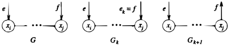
Lemma 10 Let g be any dag, and let x; and Xj be any pair of nodes such that there is a directed path from x; to Xj in 9. Let 9' be any dag equivalent to 9. For any pair of edges e E 8; (Q, 9') and f E 8i (9, 9'), e comes before f in £(9, 9').

Proof: (See Figure 1) Without loss of generality, let Xj be the first descendant of x; that has an incident edge f reversed. Let 9k be the graph in which f is reversed, or equivalently, let k be the index such that ek = f .

Assume the lemma does not hold, and hence f is re­ versed before e. Because Xj is the first descendant to have an incident edge reversed, it follows that any di­ rected path from x; to Xj in 9 must still exist in 9k. and therefore x; is an ancestor of Xj in 9k· Because f is the next edge to be reversed, it follows from Lemma 9 that 8;(9k, 9') is empty. But by assumption e has not yet been reversed in gk. and hence e � 8;(Qk, 9'), yielding a contradiction. 0

Lemma 11 Let g be any dag, and let Ry be any set of edges incident into node y such that Ry � Rg. Then there exists a dag 9' � 9 for which all edges in Ry are simultaneously reversed.

_a

Figure 1: Relevant dags for the proof of Lemma 10

Proof: (See Figure 2) Proof by induction on IRvl· For IRvl = 1, the lemma holds trivially by definition of Rg.

Assume the lemma holds for IRvl = kl.We now show the lemma holds for IRvl = k. By the induction hypothesis, there must exist a dag 1l � 9 in which k -1 of the edges from R y are reversed. Let R?t be the corresponding set of reversed edges in 1{., and let e be the edge in Ry that is not reversed in 1{.. By definition of Rg, we know there exists some dag 1{.' � 9 for which the edge e is reversed.

Because all of the edges in R?t are incident into descen­ dants of y in 1{., it follows from Lemma 10 that e comes before any edge from R?t in the sequence £(1f., 1f.'). This implies that the graph from V(1f., 1f.') that re­ sults from reversing e satisfies the stated requirements for 9'. 0

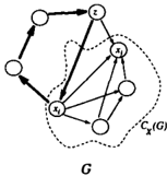
For any dag 9, we use Cx(9) to denote the subgraph of 9 induced by the nodes in set X. A clique in a directed graph 9 is a subgraph Cx(Q) such that for every pair of nodes x; and Xj in X, either the edge x; � x j or the edge x j � x; is in 9. A covered clique in a directed graph 9 is a clique Cx(Q) such that for any node z rt. X that is a parent of some node in X, z is a parent of every node in X. Note that a covered edge is a covered clique with two nodes.

Lemma 12 Let 9 be any dag containing a covered clique Cx(9). No edge connecting a pair of nodes in X can participate in a v-structure in g.

Proof: Suppose x;--+ Xj connects two nodes in X and participates in a v-structure. This implies there is a parent of Xj that is not adjacent to x; -and hence not a parent of x; -contradicting the fact that the nodes in X form a covered clique. 0

The following lemma is a generalization of Lemma 1.

Lemma 13 Let g be any dag containing a covered clique Cx(Q), and let rx be any total ordering over the nodes in X. Let 9' be the graph identical to g, ex­ cept the edges in Cx(9') are oriented to be consistent with rx. Then 9' is a dag that is equivalent to g.

Proof: Clearly 9' and 9 have the same skeleton. Sup­ pose there exists a v-structure in 9 that is not in Q'. This v-structure must include an edge from Cx(Q) be­ cause these are the only edges by which 9 can differ from 9'. But by Lemma 12, no such v-structure can exist.

Suppose there exists a v-structure in 9' that is not in 9. Because only edges contained within Cx(Q) have been reversed in 9, it follows that Cx(Q') must be a covered clique in 9', and again by Lemma 12 we conclude that no such v-structure can exist.

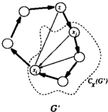
Suppose 9' contains a cycle (see Figure 3). Because 9 is acyclic, any cycle in 9' must pass through an edge in Cx (9'). Because these edges are consistent with the total ordering rx, no cycle can be completely con­ tained within Cx(9'). This implies there exists a pair of nodes x; and Xj in X such that there is a directed path from x; to Xj along the cycle in 9' consisting of no edges from Cx(9). Let z be the last node in such a path. By definition of a covered clique, z must be a parent of x; in 9, and therefore 9 contains a cycle. 0

Lemma 14 Let 9 be any dag, and let Ry = { x1 --+ y, . . . , Xk --+ y} be any subset of edges incident into node y such that Ry � Rg, and let X = { x 1 , . . . ,xk} be the set of tails of these edges. There exists a dag 9' � 9 for which Cxu{y} (9') is a covered clique in 9'.

Proof: By Lemma 11, we know there exists a dag 1{. � 9 such that Ry � 8y (9, 1f.). Consider the sequence V(9, 1i.), and let Q' be the dag resulting immediately after the last edge from Ry is reversed. We show that Cxu{y}(Q') is a covered clique in 9'.

First we show that Cxu{y}(Q') is a clique. By defini­ tion of X, y is adjacent to every node in X. Thus if the subgraph Cxu{y}(9') is not a clique, then there must exist some pair { x;, Xj} from X that are not adjacent. But this implies that (x;, y,xj) is a v-structure in 9, contradicting the fact that both x; � y and Xj � y are members of Rg.

To complete the proof, we must show that for any node z that is not in X U {y}, if z is a parent of any node in X U {y}, then z is a parent of every node in X U {y}. We break this task into two parts: we show that in g', ( 1) if z is a parent of y then z is a parent of every node in X and (2) if z is a parent of any node in X, then z is a parent of y.

(1) If z is a parent of y in g' then z is a parent of every node in X in g'.

Assume z is a parent of y.

We first show that z is also a parent of y in the original dag g. Suppose this is not the case, and g contains the edge y -+ z. By Lemma 10 all edges from Ry will be reversed before this edge. It follows by definition of g', however, that the last edge reversed was incident into y and hence y -+ z must exist in g', contradicting the assumption that z is a parent of y in g'.

Now we prove Part (1) by showing that z is a parent of every node x; E X. For any node x; E X, z must be adjacent to x; else the v-structure ( x; , y, z) exists in g and not g'. The edge must be oriented as z -+ x; in g', else there would be the directed cycle x; -+ z -+ y -+ x; in g'.

(2) If z is a parent of any node in X ing', then z is a parent of y in g'.

Assume z is a parent of some node x; E X in g'.

The node z must be adjacent to y, lest the v-structure (z, x;, y) exists in g' and not in g.

We now consider the two possible orientations for the edge between z and y in the original graph g. If the edge y -+ z is in g, then g must also contain x; -+ z, lest there would be a directed cycle in g. Because z is a descendent of y in g, we know from Lemma 10 that all the edges from Ry will be reversed before x; -+ z. It follows by definition of g', however, that the last edge reversed was incident into y and hence x; -+ z must also exist in g', contradicting the assumption that z is a parent of x; in g'.

It follows from the above argument that z -+ y must exist in the original dag g. Now, if y -+ z is in g', then z -+ y E Ry, contradicting the fact that z fl. X. Consequently, z must be a parent of y in g'. D

Corollary 2 Let g be any dag, and let R y = {x1 -+ y, . . . , Xk -+ y} be any set of edges incident into node y such that Ry � Rg. Let X = {x1, . . . , xk} be the set of tails of these edges. Every edge in Cxu{y}((i) is in Rg

Proof: By Lemma 14, there exists a dag g' � g for which Cxu{y}((i) is a covered clique. Let g" be iden­ tical to g', except that the edges in Cxu{y}((i) are oriented to be in the opposite direction of the corre­ sponding edges in g. By Lemma 13 it follows that g" �g. D

We can now prove Lemma 3 and Lemma 4. We restate both lemmas below, using the notation developed in this section.

Lem�a 3 Let . g be any dag and let C{x,y,z}((i) be any clzque of szze three. I f any two of the edges in C{x,y,z}((i) are in Rg, then the third one is also.

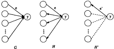
Proof: Assume that exactly two of the edges are in Rg. Without loss of generality, assume that the edge z -+ x is not in Rg . Let g' be any dag that includes the edge x -+ y. Because g' is acyclic, z -+ y is in g'. Because x -+ y and z -+ y are both both in 14;,, it follows from Corollary 2 that every edge in C {., , y ,z} ( g') is in Rg', contradicting the assumption that z -+ x is not in Rg. D

Lemma 4 Let g be any dag, and let x -+ y be any edge in g such that lly � IT., U x. The edge x -+ y is in Rg i f and only if for every edge z -+ x such that z and y are not ad jacent, z -+ x is in Rg.

Proof: (if) Assume that for every edge z -+ x such that z and y are not adjacent, z -+ x is in Rg. We now show it follows that x -+ y is reversible.

Let { z1 -+ x, . . . , Zk -+ x} � Rg be the set of all reversible edges incident into x in g, and let Z = { z 1 , . . . , Zk } be the set of tails of these edges. Let Zy C Z be the subset of nodes in Z that are parents of y (see Figure 4a).

By Lemma 14, there exists a dag g' � g for which Czu{x}((j') is a covered clique (see Figure 4b). By assumption, for every edge z -+ x such that z and y are not adjacent, z E Z \ Zy. As a result, Lemma 13 guarantees that by choosing an appropriate total ordering on the nodes in Z U { x}, we can construct a dag g" � g' such that the only edges incident into x are those that have tails in Zy (see Figure 4c).

Consider the sequence S( g, g"). By Lemma 10, ev­ ery edge in t5.,( g, g") will come before any edge from 8y ( g,g"). Let gi E V((j,g") be the dag that results after reversing the last edge in 8., ( g, g"). It follows that fl�i = Zy . Furthermore, no edge incident into y has been reversed which implies IT�; = Zy U x. Conse­ quently, x -+ y is a covered edge in gi.

(Only if) Let z -+ x be any compelled edge such that z is not adjacent to y. It follows immediately that x -+ y is compelled because any dag with x -+ y r e versed will contain the v-structure (z, x, y) that is not in g. D