Additive Belief-Network Models

Paul Dagum

Section on Medical Informatics Stanford University School of Medicine and

Rockwell Palo Alto Laboratory

444 High Street 94301

Palo Alto, California

Abstract

The inherent intractability of probabilistic in­ ference has hindered the application of be­ lief networks to large domains. Noisy OR­ gates [30] and probabilistic similarity net­ works [18, 17) escape the complexity of infer­ ence by restricting model expressiveness. Re­ cent work in the application of belief-network models to time-series analysis and forecasting [9, 10) has given rise to the additive belief­ network model (ABNM). We (1) discuss the nature and implications of the approxima­ tions made by an additive decomposition of a belief network, (2) show greater efficiency in the induction of additive models when avail­ able data are scarce, (3) generalize proba­ bilistic inference algorithms to exploit the ad­ ditive decomposition of ABNMs, ( 4) show greater efficiency of inference, and (5) com­ pare results on inference with a simple addi­ tive belief network.

1 INTRODUCTION

A Bayesian belief network is a model that employs a graphical structure to characterize a joint-probability distribution. The research that culminated in the de­ velopment of belief networks can be traced to the work of Lewis (28). Lewis addressed the problem of ap­ proximating an arbitrary distribution with low-order distributions by measuring the "goodness" of the ap­ proximation with the Kullback-Liebler cross-entropy measure [26). Subsequent research focused on meth­ ods for choosing a set of low-order distributions that best approximates the original distribution [4, 13, 25]. This research neglected the implicit dependencies and independencies that structure a domain, and instead sought to provide an approximation of the true dis­ tribution with minimal cross entropy. For domains in which structural dependencies are known, Pearl [29, 30) characterized belief networks as probabilistic models that separate structure learning, or the de­ termination of model dependencies, from parameter

Adam Galper

Section on Medical Informatics Stanford University School of Medicine Stanford, California 94305-5479

learning, or the determination of the probabilities that quantify the dependencies.

The recent development of belief-network applications [1, 2, 19, 22, 24, 32) has stimulated the maturation of techniques for probabilistic inference in belief networks and for induction of belief networks [7, 11, 23, 20, 21, 27, 30, 31). It is now evident that the intractability of available probabilistic inference algorithms hinders the application of belief networks to large domains. Both exact and approximate probabilistic inference is NP­ hard, and therefore, we do not hope to find tractable solutions to inference in large belief networks [6, 12).

The formal proofs of the complexity of inference have spurred the development of approximate modeling techniques that restrict the form of the model in or­ der to reduce the complexity of inference. Examples include noisy OR-gates [30), used in QMR-DT (32), and probabilistic similarity networks (18, 17] used in Pathfinder [19]. Motivated by recent developments in belief-network models for time-series analysis and fore­ casting [9, 10), we introduce a new approximate mod­ eling methodology: the additive belief-network model (ABNM). We (1) discuss the nature and implications of the approximations made by an additive decompo­ sition of a belief network, (2) show greater efficiency in the induction of additive models when available data are scarce, (3) generalize probabilistic inference algo­ rithms to exploit the additive decomposition of AB­ NMs ( 4) show greater efficiency of inference, and (5) compare results on inference with a simple additive belief network.

In [8], we develop a theory of algebraic belief-network models that extends the expressivity of ABNMs by al­ lowing multiplicative decompositions of a belief net­ work. For this extended class of models, we show re­ sults for learning and probabilistic inference similar to those presented here for ABNMs.

2 ADDITIVE MODEL

The theory of nonparametric additive models is rela­ tively recent [3, 14, 15). Before we define ABNMs, we discuss briefly additive models and generalized additive

models.

2.1 ADDITIVE MODELS AND GENERALIZED ADDITIVE MODELS

Suppose we desire to model the dependence of a vari­ able Y on variables X1, ... , Kp. We wish to do so for purposes of (1) description, to model the dependence of the response on the predictors in order to learn more about the process that produces Y, (2) inference, to assess the relative contribution of each predictor to Y, and (3) prediction, to predict Y given values of the predictors. When linear regression of Y on X1, ... , Xp provides an adequate model, its simplicity makes it the preferred method. The inadequacy of linear re­ gression, for example, in medical domains [16], led to the development of additive models.

Additive models maintain the attractive properties of linear-regression models; they are additive in the pre­ dictor effects, but are not constrained by assumptions of linearity in the predictor effects. An additive model is defined by

where the functions /; are arbitrary.

Generalized additive models extend additive models in the same way that generalized linear models ex­ tend linear models: they allow a general link between the predictors and the dependent variable. For exam­ ple, log-linear models for categorical data and gamma­ regression models for responses with constant coef­ ficient of variation represent generalized linear mod­ els. These generalizations extend naturally to additive models [14).

2.2 ADDITIVE BELIEF-NETWORK MODELS

We first define formally a belief-network model. A be­ lief network consists of a directed acyclic graph (DAG) and a set of conditional probability functions. Let X 1, ... , Xn represent the nodes of the DAG, and let 1r(Xi) denote the set of parents of X; in the DAG. The nodes of the DAG represent the variables of the belief network. The directed arcs in the DAG repre­ sent explicit dependencies between the variables. We assume that each variable is binary valued. To com­ plete the definition of a belief network, we specify for each variable X;, an associated conditional probability function (table) denoted Pr[X; i1r(X;)]. The full joint probability distribution is given by [30)

The key link between the theory of additive models presented in Section 2.1 and ABNMs lies in the inter­ pretation of the conditional probability functions. For node X;, specification of the function Pr[X;j7r(Xi)] im­ plies a nonparametric model of the effect of the pre­ dictors 1r(Xi) on the dependent variable X;. To make clear the analogy with additive models, we let Y de­ note X;, and we assume that 1r(X;) = {X1, ... , Xp}· We might define an additive belief-network model to be a model that satisfies

where the weights ni sum to one, and thereby nor­ malize the summation expression. Equation 1, which expresses the property of additive models, follows di­ rectly from Equation 3:

where

The expectation E[YIX;) is with respect to the distri­ bution Pr[YIX;].

We define ABNMs to be more general than additive models. We allow additive interaction terms, such as Pr[YIX;, Xj], in Equation 3. Thus, an ABNM has conditional probabilities that satisfy

where S; are subsets of the predictors such that S1 u S2 U · · · U Sk = {X1, ... , Xp}· We note that in general, it is not necessary that the S; form a disjoint parti­ tion of the predictors X 1, ... , Xp. Thus, for example, Pr[YIX;,Xj] and Pr[YIX;, Xk] might be two valid in­ teraction terms in the expression for Pr[YIX1, ... , Xp]· In Section 3, we show that it is frequently necessary to allow for nondisjoint partitions of the predictors if we are to arrive at a coherent semantics for the additive decomposition.

Whereas specification of the univariate functions in additive models is accomplished easily through a re­ cursive backfitting algorithm [16], specification of in­ teraction terms is complicated by the numerical insta­ bility and biases of the fitting procedure in higher di­ mensions. Induction of the additive interaction terms in ABNMs is relatively free of the complications we encounter in backfitting interaction terms in additive models. We discuss induction of the additive terms in ABNMs in Section 4.

3 SIGNIFICANCE OF ADDITIVE DECOMPOSITION

The decomposition of Pr[YIX1, ... , Xp] into additive terms is an approximation of the true functional de­ pendence of Y on its predictors. The decomposition

originated in the design of dynamic network models (DNMs)-belief-network models for time-series anal­ ysis and forecasting [9, 10). If the decomposition is chosen with insight, then very little is lost in the ap­ proximation. Furthermore, there is much to be gained from an additive decomposition when the number of predictors p for Y is large-as is usual in large, com­ plex domains. In Section 4, we discuss how decompo­ sition facilitates the induction of belief networks from data, and in Section 5, we show that additive decom­ position accelerates probabilistic inference. A carefully chosen additive decomposition of key conditional de­ pendencies in a belief network- even if the decompo­ sition has only two additive terms-can transform an intractable inference problem into a problem that is solved readily.

A poorly chosen decomposition, however, will intro­ duce biases into the model through assumptions about independencies among predictors. For example, the decomposition

allows us to study the dependence of Y on the pre­ dictor X 1, independent of the values of X 2, and to study the relative contribution of x1 in explaining Y. This simplicity and insight come at the expense of assuming a specific type of interaction between X 1 and x2, which at times, ma.y be sufficiently significant to bias an inference adversely. Consider the follow­ ing example modified from Pearl ( 3 0]. Let Y repre­ sent the event of "triggering an alarm", X 1 represent a "burglary", and X2 represent a "riot". We regard xl and x2 as two sources of information regarding Y, the state of the alarm. Each source provides an assessment of the alarm through the terms Pr[YjXI)

and Pr[YjX2). In an additive decomposition, we pool our sources of information through a weighted sum of the terms Pr(YIX1] and Pr(YIX2). Thus, our belief regarding the state of the alarm lies within the two extremes provided by each source of information act­ ing independently. However, if both predictors X1 and x2 are independent, then learning about a riot and a burglary should increase our belief in the alarm be­ yond the belief predicted by either source alone. In general, the additive decomposition cannot model the synergy of two independent predictors X 1 and X 2 of Y. Elsewhere [8), we show how a multiplicative decompo­ sition of conditional probabilities can model synergy between independent predictors. Furthermore, multi­ plicative decomposition, like additive decomposition, improves the efficiency of probabilistic inference and induction.

3.1 INTERCAUSAL DEPENDENCE AND ADDITIVE DECOMPOSITION

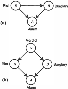
We have shown that additive decomposition should not be used when predictors are independent, but we haven't shown when an additive decomposition is ap­ propriate. Suppose a riot and a burglary are not inde­ pendent events. For example, there may be an explicit dependence, as depicted in Figure 1a, if we believe that burglaries are more likely to occur during a riot than during peaceful circumstances. A riot causes vandal­ ism that might lead to burglary, thereby triggering the alarm, or vandalism might trigger the alarm directly. Alternatively, the dependence between a riot and a burglary might be implicit, as in Figure 1b, in which the probability of a riot or a burglary is high given the jury verdict in a high-profile trial. Borrowing from Wellman and Henri on (33), we refer to explicit or im­ plicit dependence between causes of an event as in­ tercausa/ dependence. Strong intercausal dependence between predictors-for example, a high probability of burglary given a riot-reduces the confidence gained by observing both a riot and a burglary. The two in­ formation sources share background knowledge, and therefore observing both causes does not necessarily increase our confidence in the state of the alarm. The weights of the additive decomposition represent our re­ spective confidence in the two sources of information, based on, for example, the reliability of the observa­ tions, an assessment of predictive fidelity, or the con­ sistency of our background knowledge. Thus, we can use the weights to adjust for dissonant information. If we learn about the riot through an established me­ dia channel, but our information regarding burglary is third hand, we can adjust the contribution of the burglary report to our belief in the state of the alarm by discounting the weight of its prediction.

3.2 A PRESCRIPTION FOR ADDITIVE DECOMPOSITION

In summary, when the predictors {X1, ... , Xp} of Y exhibit pairwise intercausal dependence-that is, in­ tercausal dependence for any pair of predictors X; and Xj-then the additive decomposition of Equa­ tion 3 is justified. More generally, we define the in­ tercausal dependence graph for node Y to consist of nodes V = {X1, ... ,Xp} and undirected edges E de­ fined by the intercausal dependencies. When the inter­ causal dependence graph is a clique, then the additive decomposition of Equation 3 is justified. When the intercausal dependence graph is not a clique, then let {X 1, ... , X k} denote the vertices of the largest clique within the intercausal dependence graph. Let N(X;) denote the neighbor of node X; in the graph. The additive decomposition for Y is now given by Equa­ tion 4, with S; = {Xi} u (V \ N(X;)), i = 1, ... , k. The set (V \ N(X;)) denotes the predictors that are not inter causally dependent with X;.

3.3 NEGATIVE PRODUCT SYNERGY AND ADDITIVE DECOMPOSITION

A property of the additive decomposition is that the absolute contribution of a riot to the probability of trig­ gering the alarm is independent of whether or not the building is burglarized at the same time a riot occurs. A similar property holds for the absolute contribution of a burglary. In the formalism of Wellman and Hen­ rion (33], it follows that for additive decomposition, the predictors exhibit zero additive synergy with respect to Y. However, the relative contribution of a riot to the probability of triggering the alarm is dependent on whether or not the building is burglarized at the same time. More generally, it is straightforward to show for the additive decomposition that if the predictors posi­ tively influence Y, then the predictors exhibit negative product synergy with respect to Y, and this result is independent of the choice of a. In other words, under the additive decomposition, the proportional increase in the probability that the alarm rang due to learning of a riot is smaller when we know that the building was burglarized, than when we know that the building was not burglarized.

4 FITTING ADDITIVE BELIEF-NETWORK MODELS

In the additive decomposition expressed in Equation 3, we left unspecified the method of estimation of the weights Cl';. In this section, we discuss the significance of these weights and we present alternative methods for their estimation. Before we proceed, we compare the complexity of induction of the conditional prob­ abilities Pr[YjS;] with the complexity of induction of Pr[YIX1, ... ,Xp]·

4.1 INDUCTION OF CONDITIONAL PROBABILITIES

When there are many predictor variables, we may overspecify the model with insufficient data if we at­ tempt to specify Pr[YIX1, ... , Xp] directly. An over­ specified model will produce biased inferences. For example, if p = 10 and each variable has four possi­ ble values, then we must specify 2 2 0 probabilities for each value of the dependent variable Y. Not only is this beyond the realm of any domain expert, but it is clearly beyond the realm of belief-network induction algorithms [7, 31]. These algorithms induce the con­ ditional probabilities by counting cases in a database of model instantiations. To guarantee reasonable con­ vergence of the algorithm, for each instantiation of the predictors, we would like to observe at least ten cases in the database with this instantiation. Thus, we re­ quire a database of at least 107 cases-clearly a pro­ hibitive demand. On the other hand, even a single additive split of Pr[YIX1, ... , X1 0 ] into two conditional probabilities, each with five predictors, reduces sub­ stantially the number of cases required for induction. With a single decomposition, we require specification of 2 10 , or one thousand, probabilities for each value of the dependent variable, and a database of 104 cases will suffice for induction.

4.2 ESTIMATION OF PARAMETERS

In Equation 3, we argued that the weights a; were nec­ essary to normalize the sum of conditional probabili­ ties. Although the a; normalize the sum, they also af­ fect significantly each summand's relative contribution to the conditional probability Pr[YIX1, ... , Xp]. For ex­ ample, in DNMs, we decompose conditional probabil­ ities into two terms: the first term contains the sub­ set of predictors that are contemporaneous with the dependent variable Y, and the second term contains the subset of predictors that are noncontemporaneous with Y. The weights a and 1 -a in DNMs represent the relative contribution to the prediction of Y from contemporaneous and noncontemporaneous informa­ tion. A value of a near one favors the prediction of Y based on contemporaneous data, whereas a value of a near zero favors the prediction of Y based on noncon­ temporaneous data.

Fitting an ABNM refers to the specification of the weights. We view the weights as probabilities that denote the contribution of each summand to Pr[YIX 1 , ... , Xp]· We fit ABNMs through iterative Bayesian update of the weights with new evidence.

Let Pr[a1, ... , ak ] = Pr[<i] denote the probability distri­ bution for the weights. Assume that we have observed evidence that consists of m independent instantiations of the network E1, ... ,Em, with the union of this evi­ dence denoted by fm. Let Pr[nl£m] denote the prob­ ability distribution for the weights a after we observe the evidence. We update the distribution with evi-

dence Em+l according to Bayes' rule:

where Pr[Em+lla, fm] is the probability of evidence Em+l we compute with the ABNM and k normalizes the distribution.

4.3 CROSS-ENTROPY VALIDATION

To validate an ABNM, we can measure how closely the inferences generated with the ABNM approxi­ mate the inferences generated by a full belief-network model. Let Pr[Xl, ... ,Xn] and Pr'[X1, ... ,Xn] de­ note the full joint probability distributions of a be­ lief network BN and of an ABNM that approximates BN. The Kullback-Liebler cross-entropy [26] measures how well the distribution Pr'[X1, ... , Xn] approximates Pr[X1, ... ,Xn]:

We can easily show that lpr,Pr' 2: 0, and it is equal to zero only if the distributions are identical. The closer IPr , Pr' is to zero, the better Pr'[x1, ... ,xn] approxi­ mates Pr[x1, ... , Xn]. Thus, once we specify the param­ eters of the ABNM, we can construct its full joint prob­ ability and compute the cross entropy. Unfortunately, to compute the cross-entropy, we must sum over all

belief-network instantiations, and for large networks cross-entropy calculations are intractable.

The cross-entropy IPr,Pr' is a function of the parame­ ters of the ABNM. Each node with an additive decom­ position als� has an associated set of parameters. If we assume that the parameter11 of a node can be speci­ fied independently of each other and of the parameters of other nodes, then we can compute the parameters that minimize IPr,Pr'· For node X; with an additive decomposition, let Sf, ... , Si denote the additive parti­ tion of the parent nodes of X;, 11'( X;), and let ai, ... , ak denote the parameters of the additive decomposition. (The number of terms k in the partition may vary across nodes.) We use Equations 2 and 3 to express the cross entropy given by Equation 5 as

where the the second sum in this expression is over all instantiations of node X; and its parents 11'(Xi). Each term I; is a function of the parameters for node X; only. We compute the parameters which minimize the cross entropy by solving for a) in

for all i and j. Using the expression for I; in Equation 6 d . 1 "\' k-1 an smce ak = -i..J j = l aj, we get

Solution of Equation 7 is a difficult task when the number of parameters I is large. We must search the /-dimensional unit cube for the solutions of this equa­ tion. Fortunately, I is often small. Furthermore, to solve Equation 7 we must compute the probabilities Pr[x;, 11'(X;)] for all instantiations of x; and 1r(X;). In the worst case these probabilities cannot be computed exactly, and we must approximate them with a sim­ ulation algorithm. Nontheless, in many cases we can solve Equation 7 exactly to yield a set of parameters that minimizes the cross entropy between the full joint probabilities of BN and ABNM.

5 INFERENCE ALGORITHM

Both exact and approximate probabilistic inference in belief networks is NP-hard [6, 12], and therefore, in­ tractable for sufficiently large belief networks. In this section, we develop an exact inference algorithm for ABNMs that exploits the additive decomposition. The run time of the algorithm depends on the decomposi­ tion of the ABNM, however, when we chose the decom­ positions thoughtfully, we render inference tractable in all cases.

The inference algorithm we present is similar to Cooper's nested dissection algorithm for probabilistic inference [5]. We decompose the belief network into subnetworks using the additive decomposition. We use the Lauritzen-Speiglehalter (L-S) algorithm [27] to perform inference on the subnetworks. The decom­ position renders the subnetworks amenable to fast in­ ference with the 1-S algorithm. We then combine the results from each subnetwork inference to arrive at the desired inference probability.

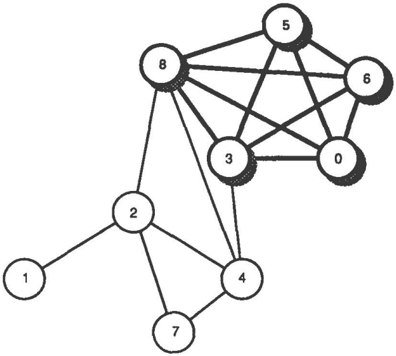
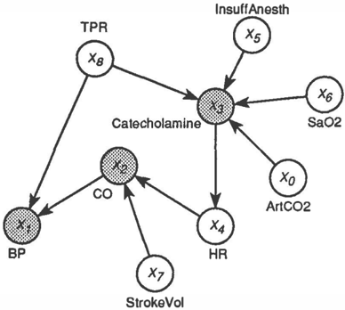
We introduce the algorithm through an example. We; assume familiarity with the 1-S algorithm. Figure 2 gives a portion of ALARM [2], a belief network for pa­ tient monitoring in an intensive care unit; we call this subnetwork AlarmX. The L-S algorithm first builds a triangulated graph composed of cliques. Figure 3 shows the triangulated graph and shadows the nodes contained in the largest clique Co: {xo, X3, xs, X6, xs}. The algorithm constructs clique marginals for each clique. The clique marginals are probability distribu­ tions over all nodes of the clique-for example, the clique marginal for Co is the probability distribution Pr[xo, X3, xs, X6, xs]. For each clique, the 1-S algo­ rithm stores the table of clique marginals over all in­ stantiations of the nodes in the clique. Thus, if d; denotes the number of values assumed by each node X; in the belief network, then for a clique C comprised of nodes x1, ... , Xk, the algorithm must store a table of clique marginal probabilities of size

-

If each node in Co has five possible values, the the 1-S algorithm stores a table of clique marginals for Co of size 5 5 = 3125. The running time of the 1-S algorithm is proportional to N (C), evaluated at the largest clique c.

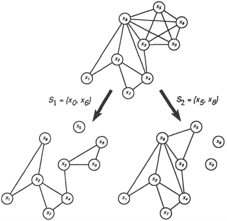
Nodes x1, x2, and x3 are assumed to have the ad­ ditive decompositions shown. The ABNM inference algorithm selects a decomposable node contained in the largest clique. The algorithm chooses x3 in the example. The algorithm dissects the belief network at the chosen node to generate two belief networks BNa and BN1-a· BNa is obtained from BN by deleting the edges from nodes X 5 and xs to node X3. BN 1-a is ob­ tained from BN by deleting the edges from nodes xo and X6 to node X3. BNa and BN 1-a and the corre­ sponding triangulated graphs are shown in Figure 4. We observe that a single dissection reduces N(C) from 3125 for BN, to 125 for both BNa and BN1-a· If we want to compute the inference Pr[x6lxi], we use the 1S algorithm to compute the inferences Pra[x61xi] and

Pr1-a(x6lx1] in BNa and BN1-a, respectively. We can verify readily that

Pr(x61xd = aPra(x61xt] + (1- a)Prl-a(x61xl]· We have reduced storage and computation from 3125 clique marginal probabilities to two tables of 125 prob­ abilities.

We could continue to dissect both BNa and BN1-a at either x1 or x2· The process is identical, and if we were to dissect along all three nodes, we would gen­ erate eight sparse belief subnetworks. As a rule, how­ ever, we only dissect a node if it reduces the size of the largest clique. Thus, we avoid generating a large num­ ber of sparse belief subnetworks that we must store and evaluate each time we compute an inference.

6 IMPLEMENTATION RESULTS

We implemented our probabilistic inference algorithm for ABNMs. We present here results for AlarmX. To highlight the effects on the complexity of inference and on the cross entropy between the full joint probabili­ ties, we assume that node x3 is the only decomposable node.

To obtain the prior conditional proba­ bilities Pr(:z:3l:z:o, x6] and Pr(x3jx5, :z:s] for AlarmX, we marginalized the conditional probability for :z:3 in the full model. In general, we would assess these proba­ bilities directly from the expert, or induce them from data by counting fractional occurences of the instanti­ ations. The weight a3 denotes the contribution from Pr(:z:3l:z:o, x6] to the conditional probability for :z:3, and 1- a3 denotes the contribution from Pr(x3jx5, x8].

When a3 = 0.485, we obtain the minimum value for the cross entropy, Ipr Pr ' = 0.311079. Recall that the cross entropy ranges f � om 0 to infinity, and it is identi­ cally zero if the two probability distributions are iden­ tical.

We compare the marginal probabilities we obtain with the full belief network and the ABNM for AlarmX. These probabilities were identical for ali the nodes ex­ cept node X 1 · The full belief network gives marginal probabilities of 0.4444, 0.2723, and 0.2834, correspond­ ing to a value of Low, Medium, and High for node X 1. For the same node, the ABNM gives marginal proba­ bilities 0.4425, 0.2606, and 0.2969.

7 CONCLUSIONS

Like noisy-OR models and probabilistic similarity net­ works, ABNMs are approximate models that trade off predictive accuracy for speed and simplicity. Unlike the other methodologies, however, the ABNM method­ ology does not make as stringent an assumption about model structures or probabilities. When faced with a large, complex domain, a modeler can iteratively re­ fine an ABNM by partitioning nodes that contribute significantly to intractability.

We have discussed the properties of ABNMs and have provided means for the estimation of their parameters. We have measured how well ABNMs model a domain by the cross entropy between the full joint probabili­ ties of the ABNM and the full belief network. In an example ABNM, we found that the cross entropy was 0.311, and therefore, the ABNM provided a compara­ ble model of the domain. Furthermore, the complexity of inference in the ABNM for our example was reduced by one order of magnitude. Future research objectives include ( 1) the development of search strategies for the partition that minimizes the cross entropy between the ABNM and the full belief network, (2) the extension of ABNMs to log-linear models (8], and (3) further tests and validation of the methodology.

Acknowledgments

This work was supported by the National Science Foundation under grant IRI-9108385, by Rockwell International Science Center IR&D funds, and by the Stanford University CAMIS project under grant IP41LM05305 from the National Library of Medicine of the National Institutes of Health.

References

• (1] S. Andreassen, M. Woldbye, B. Falck, and S.K. Andersen. Munin- a causal probabilistic network for interpretation of electromyographic findings. In Proceedings of 1Oth International Joint Confer­ ence on Artificial Intelligence, Milan, Italy, 1987.
• (2] I. Beinlich, H. Suermondt, R. Chavez, and G. Cooper. The ALARM monitoring system: A case study with two probabilistic inference tech­ niques for belief networks. In Proceedings of the Second European Conference on Artificial Intelli­ gence, Berlin, 1989. Springer-Verlag.
• (3] A. Buja, T. Hastie, and R. Tibshirani. Linear smoothers and additive models (with discussion). Ann. Statist., 17:453-555, 1989.
• (4] P. Cheeseman. A method of computing gener­ alized Bayesian probability values for expert sys­ tems. In Proceedings of the 8th International Joint Conference on Artificial Intelligence, pages 198202, August 1983.
• (5] G. Cooper. Bayesian belief-network inference us­ ing nested dissection. Technical Report KSL90-05, Knowledge Systems Laboratory, Stanford University, Stanford, CA, February 1990.
• (6] G. Cooper. The computational complexity of probabilistic inference using Bayesian belief net­ works. Artificial Intelligence, 42:393-405, 1990.
• (7] G. Cooper and E. Herskovits. A Bayesian method for the induction of probabilistic networks from data. Machine Learning, 9:309-347, 1992.

1. P. Dagum and A. Galper. Algebraic belief net­ work models: Inference and induction. Technical Report KSL-93, Knowledge Systems Laboratory, Stanford University, Stanford, CA, May 1993.
2. P. Dagum, A. Gal per, and E. Horvitz. Dynamic network models for forecasting. In Proceedings of the Eighth Workshop on Uncertainty in Artifi­ cial Intelligence, pages 41-48, Stanford, CA, July 1992. American Association for Artificial Intelli­ gence.
3. P. Dagum, A. Gal per, and E. Horvitz. Dynamic network models for temporal probabilistic rea­ soning. Technical Report KSL-91-64, Section on Medical Informatics, Stanford University, Stan­ ford, CA, 1992. Under review for Pattern Analy­ sis and Machine Intelligence.
4. (11] P. Dagum and E. Horvitz. A Bayesian analysis of simulation algorithms for inference in belief net­ works. Networks, 1992. In press.
5. P. Dagum and M. Luby. Approximating prob­ abilistic inference in Bayesian belief networks is NP-hard. Artificial Intelligence, 60:141-153, 1993.
6. S. Goldman and R. Rivest. A non-iterative maxi­ mum entropy algorithm. In Uncertainty in Ar­ tificial Intelligence. Elsevier Science Publishers, 1988.
7. T. Hastie and R. Tibshirani. Generalized addi­ tive models (with discussion). Statistical Science, 1:297-318, 1986.
8. T. Hastie and R. Tibshirani. Generalized additive models: some applications. Journal of the Amer­ ican Statistical Association, 82:371-386, 1987.
9. T. J. Hastie and R. J. Tibshirani. Generalized Additive Models. Monographs on Statistics and Applied Probability 43. Chapman and Hall, New York, 1990.
10. (17] D. Heckerman. Probabilistic similarity networks. PhD thesis, Departments of Computer Science and Medicine, Stanford University, Stanford, CA, 1990.
11. D. Heckerman. A tractable algorithm for diagnos­ ing multiple diseases. In Uncertainty in Artificial Intelligence 5, pages 163-171. Elsevier, Amster­ dam, The Netherlands, 1990.
12. D.E. Heckerman, E.J. Horvitz, and B.N. Nath­ wani. Toward normative expert systems: The Pathfinder project. Methods of Information in Medicine, 1992.
13. M. Henrion. Towards efficient inference in mul­ tiply connected belief networks. In Influence di­ agrams, belief nets, and decision analysis. John Wiley and Sons, Chichester, UK, 1990. 385-407.
14. M. Henrion. Search-based methods to bound di­ agnostic probabilities in very large belief nets. In
15. Proceedings of the Seventh Workshop on Uncer­ tainty in Artificial Intelligence, University of Los Angeles, Los Angeles, CA, July 1991. American Association for Artificial Intelligence.
16. M. Henrion, J .S. Breese, and E.J. Horvitz. Deci­ sion analysis and expert systems. AI Magazine, 12:64-91, 1992.
17. E. Herskovits. Computer-based Construction of Probabilistic Networks. PhD thesis, Program in Medical Information Sciences, Stanford Univer­ sity, Stanford, CA, 1991.
18. E. J. Horvitz, J. S. Breese, and M. Henrion. Deci­ sion theory in expert systems and artificial intelli­ gence. Journal of Approximate Reasoning, 2:247302, 1988.
19. H. Ku and S. Kullback. Approximating discrete probability distributions. IEEE Transactions on Information Theory, IT-15(4):444-447,July 1969.
20. S. Kullback and R. A. Leibler. Information and sufficiency. Annals of Mathematical Statistics, pages 79-86, 1951.
21. S. Lauritzen and D. Spiegelhalter. Local compu­ tations with probabilities on graphical structures and their application to· expert systems. Journal of the Royal Statistical Society B, 50(19), 1988.
22. P. M. Lewis. Approximating probability distribu­ tions to reduce storage requirements. Information and Control, 2:214-225, 1959.
23. (29] J. Pearl. Fusion, propagation, and structuring in belief networks. Artificial Intelligence, 29:241288, 1986.
24. J. Pearl. Probabilistic reasoning in intelligent sys­ tems: Networks of plausible inference. Morgan Kaufmann, San Mateo, CA, 1988.
25. J. Pearl and T. Verma. A theory of inferred cau­ sation. In Principles of Knowledge Representa­ tion and Reasoning: Proceedings of the Second International Conference, pages 441-452. Morgan Kaufmann, April 1991.
26. M. Shwe, B. Middleton, D. Heckerman, M. Hen­ rion, E. Horvitz, H. Lehmann, and G. Cooper. A probabilistic reformulation of the QUICK MED­ ICAL REFERENCE system. In Proceedings of the Fourteenth Annual Symposium on Computer Ap­ plications in Medical Care, pages 790-794, Wash­ ington, D.C., 1990. The American Medical Infor­ matics Association.
27. (33] M. Wellman and M. Henrion. Qualitative inter­ causal relations, or explaining "explaining away". In Principles of Knowledge Representation and Reasoning: Proceedings of the Second Interna­ tional Conference, pages 535-546. April 1991.