An Importance Sampling Algorithm Based on Evidence Pre-propagation

Changhe Yuan and Marek J. Druzdzel

Decision Systems Laboratory School of Information Sciences and Intelligent Systems Program University of Pittsburgh Pittsburgh, PA 15260 [email protected], [email protected]

Abstract

Precision achieved by stochastic sampling al­ gorithms for Bayesian networks typically de­ teriorates in face of extremely unlikely ev­ idence. To address this problem, we pro­ pose the Evidence Pre-propagation Impor­ tance Sampling algorithm (EPIS-BN), an importance sampling algorithm that com­ putes an approximate importance function using two techniques: loopy belief propaga­ tion [19, 25] and E-cutoff heuristic [2]. We tested the performance of EPIS-BN on three large real Bayesian networks: ANDES [3], CPCS [21], and PATHFINDER [11]. We observed that on each of these networks the EPIS-BN algorithm outperforms AIS­ BN [2], the current state of the art algorithm, while avoiding its costly learning stage.

1 Introduction

Bayesian networks model explicitly probabilistic inde­ pendence relations among sets of variables. By factor­ izing a full joint distribution over a set of variables into a product of conditional distributions, a Bayesian net­ work dramatically reduces the number of parameters that are required to represent this distribution. How­ ever, exact inference in Bayesian networks is still worst case NP-hard [4]. Although approximate inference to any desired precision is worst-case NP-hard as well [5], it is the only feasible alternative for sufficiently large and densely connected networks.

A prominent subclass of approximate inference algo­ rithms are stochastic sampling algorithms. Some of these are probabilistic logic sampling [12], likelihood weighting [6, 24], backward sampling [7], and impor­ tance sampling [24]. A subclass of stochastic sampling methods, called Markov Chain Monte Carlo {MCMC)

methods, includes Gibbs sampling, Metropolis sam­ pling, and Hybrid Monte Carlo sampling [8, 10, 17]. Stochastic sampling algorithms work well in predictive inference, but for diagnostic reasoning, especially with unlikely evidence, they often fail to provide good re­ sults within limited resources. However, given a good importance function, importance sampling algorithms may yield excellent approximate posteriors in a reason­ able time. Researchers already proposed some meth­ ods for pre-computing good importance functions, such as those in the AIS-BN algorithm [2], the IS algo­ rithm [14], and the IS_T algorithm [23]. In this pa­ per, we propose a new importance sampling algorithm, which we call Evidence Pre-propagation Importance Sampling algorithm for Bayesian Networks (EPIS­ BN). In this algorithm, we first use loopy belief prop­ agation to compute an approximation of the optimal importance function, and then apply E-cutoff heuristic to cut off small probabilities in the importance func­ tion. We test the EPIS-BN algorithm on several large real Bayesian networks and compare the results with the AIS-BN algorithm. The empirical results show that the EPIS-BN algorithm provides a considerable improvement over the AIS-BN algorithm, especially in those cases that are hard for the latter.

The outline of the paper is as follows. In Section 2, we give a general introduction to importance sampling. We also summarize the main idea of one of its varia­ tion, the AIS-BN algorithm, which is the current state of the art algorithm and with which we later compare the EPIS-BN algorithm. In Section 3, we discuss the EPIS-BN algorithm. First, we give an introduction to loopy belief propagation algorithm and then explain how the EPIS-BN algorithm uses it to calculate an importance function. After that, we present the details of the EPIS-BN algorithm. In Section 4, we describe the results of experimental tests of the EPIS-BN algo­ rithm on several large real Bayesian networks. Finally, in Section 5, we summarize our results, and then sug­ gest several possible further research topics.

2 Importance Sampling in Bayesian Networks

We feel that it is necessary to take a look at the the­ oretical roots of importance sampling. Let f(X) be a function of n variables X= (X1, ... ,Xn) over do­ main n c Rn. Consider the problem of estimating the multiple integral

We assume that the domain of integration of f(X) is bounded, i.e., that I exists. Importance sampling approaches this problem by estimating

where g(X), which is called the importance function, is a probability density function such that g(X) > 0 for any X c n. g(X) should be easy to sample from. In order to estimate the integral, we generate samples Xt, x2, . . . , XN from g(X) and use the generated values in the sample-mean formula

Importance sampling assigns more weight to regions where f(X) > g(X) and less weight to regions where f(X) < g(X) to correctly estimate I. It is easy to see from Eq. 2 that �f�l is an unbiased estimator of I. Rubinstein [22] points out that if f(X) > 0, the optimal importance function is

However, finding I is equivalent to solving the integral, so the method appears useless. But if we can find a function that is close enough to the optimal importance function, we can still expect good convergence rate. To get a better convergence rate, it is also important, as noted by Geweke [9], that the tails of g(X) do not decay faster than the tails of !({). Otherwise, the convergence rate will be slow.

Since it is impossible to get the optimal importance function, we should set a good importance function as our goal. Cheng & Druzdzel [2] proposed a method to calculate such an importance function in the AIS-BN algorithm. Empirical results showed that the AIS­ BN algorithm achieved over two orders of magnitude improvement in convergence over likelihood weighting and s elf-importance sampling. The improvement came mainly from two heuristics: ( 1) initializing the proba­ bility distributions of parents of evidence nodes to uni­ form distribution, and (2) adjusting very small proba­ bilities in the conditional probability tables. In addi­ tion to these two heuristics, the AIS-BN algorithm adopts an importance function learning step to ap­ proach the optimal importance function.

Although the two heuristics are cleverly designed, they themselves do not lead to a good importance function, but rather accelerate the importance function learning step, which is rather time consuming. In addition, the learned importance function may decay faster than the tails of the optimal importance function. In this paper, we propose an algorithm that directly computes an approximation of the optimal importance function rather than learning it.

3 EPIS-BN: Evidence Pre-propagation Importance Sampling Algorithm

In predictive inference, since both evidence and soft evidence are in the roots of the network, stochastic sampling can easily reach high precision. However, in diagnostic reasoning, especially when the evidence is extremely unlikely, sampling algorithms can exhibit a mismatch between the sampling distribution and the posterior distribution. In such cases most samples may be incompatible with the evidence and be useless. Some stochastic sampling algorithms such as likelihood weighting and importance sampling try to make use of all the samples by assigning weights for them. But most of the weights turn out to be too small to be effective. Backward sampling [7] tries to deal with this problem by sampling backward from the evidence nodes, but it may fail to consider the soft evidence in the roots [23]. Whatever sampling order is chosen, a good importance function has to take into account the information ahead in the network. If we do sampling in the topological order of the network, we need an importance function that will match the information from the evidence nodes. In the EPIS-BN algorithm, we make use of the loopy belief propagation to calculate such an importance function.

3.1 Loopy Belief Propagation

The goal of the belief propagation algorithm [20] is to find the posterior beliefs of each node X, i.e., BEL(x) = P(X = x j E ) , where E denotes the set of evidence. In a polytree, any node X d-separates E into two subsets E+, the evidence connected to the parents of X, and E-, the evidence connected to the children of X. Given the state of X, the two subsets are independent. Therefore, node X can collect mes­ sages separately from them in order to compute its

posterior beliefs. The message from £+ is defined as

By decomposing 1r(x) and >.(x) into more detailed messages between neighboring nodes, we can calculate 1r(x) and >.(x) for all the nodes by propagating mes­ sages throughout the network. [20] gives the details about how to calculate the messages. After we get the messages, we can compute the posterior beliefs of X by

With slight modifications, we can apply Pearl's be­ lief propagation algorithm to networks with loops. The resulting algorithm is called loopy belief propa­ gation [19, 25]. In general, loopy belief propaga­ tion will not give the correct posteriors for networks with loops. However, recently researchers performed extensive investigations on the performance of loopy belief propagation, and reported surprisingly accurate results [1, 18, 19, 25]. As of now, more thorough un­ derstanding of why the results are so good has yet to be developed. For our purpose of getting an approxi­ mate importance function, whether or not loopy belief propagation converges to the correct posteriors is not critical.

3.2 The EPIS-BN Algorithm

Let X= {X1,X2, ... ,Xn} be the set of variables in a Bayesian network, P A(Xi) be the parents of Xi, E be the set of evidence. Based on the theoretical considerations in Section 2, we know that the optimal importance function is

After factorizing P(X]E), we get

where each P(Xi]PA(Xi),E) is defined as importance conditional probability table (I CPT) [2].

Definition 1 A n importance conditional probability table (!CPT) of a node Xi is a table of posterior prob­ abilities P(Xi]P A(Xi), E) conditional on the evidence and indexed by its immediate predecessors, P A(Xi).

The AIS-BN [2] algorithm adopts a long learning step to learn approximations of these ICPTs, and hence the importance function. The following theorem shows that in polytrees we can calculate them directly.

and the message from Eis defined as

Theorem 1 Let Xi be a variable in a polytree, and E be the set of evidence. The exact !CPT P(Xi]P A(Xi), E) for Xi is

where a(P A( X;)) is a normalizing constant dependent on PA(X;).

Proof: Let E = E+ U E-, where E+ is the evidence connected to the parents of Xi, and Eis the evidence connected to the children of Xi, then

Given Theorem 1 and Eq. 9, we have the following corollary.

Corollary 1 For a polytree, the optimal importance function is

If a node has no descendant with evidence, its ICPT is identical to its CPT. This property is also explained in Theorem 2 in [2].

In networks with loops, getting the exact >. messages for all variables is equivalent to calculating the exact solutions, which is an NP-hard problem. However, because our goal is to obtain a good, not necessar­ ily optimal importance function, we can satisfy it by calculating approximations of the >. messages. Given the surprisingly good performance of loopy belief prop­ agation, we believe it can also provide us with good approximate >. messages.

Another heuristic method that we use in EPIS-BN is -cutoff [2], i.e., setting some threshold and re� placing any smaller probability in the network by . At the same time, we compensate for this change by subtracting it from the largest probability in the same conditional probability distribution. This method is originally used in AIS-BN to speed up its importance function learning step [2]. We use it for a different pur� pose. Since we use approximate messages to calculate the importance function, we are likely to violate the requirement that the tails of our importance function do not decay faster than the optimal importance func� tion. We try to satisfy this requirement by adjusting

the small probabilities in our ICPTs. However, the optimal threshold value is highly network dependent. Furthermore, if the calculated importance function al­ ready satisfies this requirement, we may get worse im­ portance function if we still apply £-cutoff .

1. Order the nodes according to their topological order.
2. Initialize parmaters m ( number of samples ) , E and d ( propagation length ) .
3. Initialize the messages that all evidence nodes send to themselves to be vectors of a 1 for the observed state and O's for other states, and all other messages to be uniformly vectors of 1 's.
4. for i <--1 to d do
5. For all of the nodes, recompute their new outgoing messages based on the incoming messages from the last iteration for all of the nodes.

end for

1. Calculate the importance function based on the final messages.
2. Enhance the importance function by the £-cutoff heuristic.
3. for i <--1 to m do
4. si <--generate a sample according to P(X]E)
5. Compute the importance score WiScore of Si.
6. Add WiScore to the corresponding entry of each score table.

end for

1. Normalize each score table, output the estimated beliefs for each node.

Figure 1: The Evidence Pre-propagation Importance Sampling Algorithm for Bayesian Networks ( EPIS­ BN ) .

The basic EPIS-BN algorithm is outlined in Figure 1. The parameter m, the number of samples, is a matter of tradeoff between precision and time. More samples will lead to a better precision. However, the optimal values of the propagation length d and the threshold value E for £-cutoff are highly network dependent. We will recommend some values bases on our empirical results in Section 4.2.

4 Experimental Results

To test the performance of the EPIS-BN algorithm, we applied it to several large real Bayesian networks, and compared our results to those of AIS-BN, the cur­ rent state of the art algorithm. This section presents the results of our experiments. We implemented our algorithm in C++ and performed our tests on a Pen­ tium III, 733 MHz Windows XP computer.

4.1 Experimental Method

To compare the accuracy of sampling algorithms, we compare their departure from the exact solutions, which we calculate using the clustering algorithm [16]. The distance metric we use is Hellinger's distance [15]. Hellinger's distance between two distributions f 1 and f2, which have probabilities Pl(Xij) and Pz(Xij) for state j (j = 1, 2, ... , ni) of node i respectively, such that Xi � E is defined as:

where N is the set of all nodes in the network, E is the set of evidence nodes, and ni is the number of states for node i.

Hellinger's distance weights small absolute probabil­ ity differences near 0 much more heavily than sim­ ilar probability differences near 1. In many cases, Hellinger's distance provides results that are equiva­ lent to Kullback-Leibler measure. However, a major advantage of Hellinger's distance is that it can han­ dle zero probabilities, which are common in Bayesian networks. For comparison purpose, in some results we also report the Mean Square Error ( MSE ) .

4.2 Parameter Selection

The most important tunable parameter in our algo­ rithm is the propagation length d. Since we are using loopy belief propagation only to get the approximate .\ messages, we need not wait until loopy belief prop­ agation converges. We can simply adopt a propaga­ tion length equal to the depth of the deepest evidence node. However, two problems arise here. First, usu­ ally the influence of evidence on a node attenuates as the distance of the node from the evidence becomes longer [13]. Therefore, we can save a lot of effort if we stop the propagation process after a small number of iterations. Second, for networks with loops, we would

be able to avoid double counting of evidence by stop­ ping propagation after a number of iterations that is less than the size of the smallest loop [25].

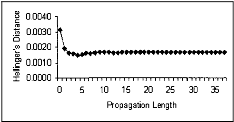
Figure 2 shows an experiment that we conducted to test the influence of propagation length on precision of the results in the ANDES network [3]. Other net­ works yielded similar results. In this case, we ran­ domly selected 20 evidence nodes for the ANDES net­ work. After performing different number of iterations of loopy belief propagation, we ran the EPIS-BN algo­ rithm and generated 320K samples. The results show that a length of 2 is already sufficient to yield very good results. Increasing the propagation length to 5 improves the results minimally. Further propagation can even make the results worse. Although for differ­ ent networks and evidence, the optimal propagation length was different, our experiments showed that the lengths of 4 or 5 were sufficient for deep networks. For shallow networks, we chose the depth of the deepest evidence as the propagation length.

Another important parameter in EPIS-BN is the threshold value for -cutoff The optimal value for is also network dependent. Our empirical tests did not yield a universally optimal value, but we recom� mend to use = 0.006 for nodes with the number of outcomes fewer than 5, and = 0.001 for nodes with the number of outcomes between 5 and 8. Otherwise, we recommend equal to 0.0005. These recommenda� tions are different from those in [2]. The main reason for this difference is that the E-cutoffis used at a differ� ent stage of the algorithm and for a different purpose.

4.3 Results for the ANDES Network

The main network we used to test our algorithm on was one of the ANDES networks [3], consisting of 233 nodes. This network has a large depth and high con- nectivity and it was shown to be difficult for the AIS­ BN algorithm [2].

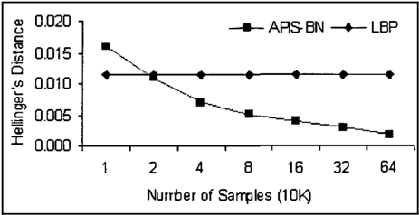
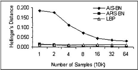
Figure 3 shows a typical result of our experiments on the convergence rate of the AIS-BN algorithm and the EPIS-BN algorithm. Figure 4 shows the result of EPIS-BN on a finer scale. In this case, we chose the propagation length to be 5 for EPIS-BN, and ran­ domly selected 20 evidence for the ANDES network. The prior probability of evidence was, similarly to the tests performed in [2], typically between w- IO and w- 40 · We also report the results of 100 iterations of loopy belief propagation. The results show that EPIS­ BN achieved a precision near one order of magnitude higher than AIS-BN, while AIS-BN performed even worse than loopy belief propagation. Our comparison was based on the number of samples. However, AIS­ BN has a long learning step, which took about 7.7 sec­ onds for the ANDES network. EPIS-BN took only 0.5 second to do belief propagation. Relative to the sampling time, which was about 30 seconds when the number of samples is 320K, they really made a dif­ ference. If we take into account this time discrepancy, EPIS-BN can achieve even better performance within

the same time. In the tables below, we do not include these times.

Table 1: Summary of the simulation results for all the 75 simulation cases on the ANDES network. H stands for Hellinger's distance, and M for MSE.

	EPIS(H)	AIS(H)	EPIS(M)	AIS(M)
J1.	0.0029	0.0590	0.0034	0.0739
(5	0.0012	0.0504	0.0014	0.0636
min	0.0010	0.0021	0.0012	0.0025
median	0.0026	0.0437	0.0031	0.0560
max	0.0065	0.2188	0.0079	0.2776

We generated a total of 75 test cases on the AN­ DES network. These cases consisted of five sequences of 15 cases each. For each sequence, we randomly chose a different number of evidence nodes: 15, 20, 25, 30, 35 respectively. The evidence nodes were cho­ sen from a predefined list of potential evidence nodes. In each test case, we set the propagation length to be 5, and ran both EPIS-BN and AIS-BN on the net­ work for 320K samples. Table 1 summarizes these 75 test cases. It shows that EPIS-BN was significantly better than AIS-BN. The results of a paired one-tailed t-test for Hellinger's distance and MSE are 3.24E- 15 and 4.01E- 15 respectively. They show us highly sig­ nificant difference between EPIS-BN and AIS-BN on the ANDES network.

4.4 Results for Other Networks

In addition to the ANDES network, we also tested EPIS-BN on two other networks, CPCS [21] and PATHFINDER [11]. Although the results were not as spectacular as those on the ANDES network, we still observed improvement.

The CPCS (Computer-based patient Case Study) net­ war k is a model representing a subset of the domain of internal medicine. It has many small probabilities, typically on the order of w- 4 . The version we used had 179 variables, a subset of the full version.

Table 2: Summary of the simulation results for all the 75 simulation cases on the CPCS network. H stands for Hellinger's distance, and M for MSE.

	EPIS(H)	AIS(H)	EPIS(M)	AIS(M)
J1.	0.00080	0.00097	0.00060	0.00076
(5	0.00020	0.00046	0.00016	0.00034
min	0.00062	0.00064	0.00030	0.00037
median	0.00073	0.00084	0.00057	0.00068
max	0.00183	0.00386	0.00142	0.00255

We also generated 75 test cases on the CPCS network by the same experiment. The only difference is that since the CPCS network is a relatively shallow net­ work, we dynamically set the propagation length to be the depth of the deepest evidence. Most of the po­ tential evidence nodes are leaf nodes in the network. Here also, the prior probability of evidence was ex­ tremely small, between w- !O and w- 40 with a me­ dian of w- 25 . The learning overhead of AIS-BN was 5.4 seconds, while the loopy belief propagation took only 0.4 second for EPIS-BN. The sampling step cost about 25 seconds. Table 2 summarizes the 75 test cases on the CPCS network.

Table 3: Summary of the simulation results for all the 75 simulation cases on the PATHFINDER network. H stands for Hellinger's distance, and M for MSE.

	EPIS(H)	AIS(H)	EPIS(M)	AIS(M)
J1.	0.00072	0.00077	0.00036	0.00039
(5	0.00021	0.00033	0.00011	0.00014
min	0.00034	0.00039	0.00021	0.00020
median	0.00067	0.00070	0.00034	0.00037
max	0.00178	0.00263	0.00076	0.00121

The third large real network that we used in our tests is the PATHFINDER network [11]. The version we used consists of 135 nodes. Since the PATHFINDER network has many probabilities that are equal to 1 and 0, we hit zero probability evidence sometimes when generating a test case. So we ran the experiment multiple times, and collected the first 75 effective test cases, in which the generated evidence had non-zero probability. The learning overhead for AIS-BN was 3.5 second, while only 0.3 second for EPIS-BN. The sampling step cost about 15 seconds. Table 3 summarizes the 75 test cases for the PATHFINDER network.

The improvement of the EPIS-BN algorithm over the AIS-BN algorithm for the CPCS network and the PATHFINDER network is smaller than that for the AN­ DES network. To test whether this smaller difference is due to the ceiling effect, we performed experiments on these networks without evidence. When no evi­ dence is present, both EPIS-BN and AIS-BN reduce to probabilistic logic sampling [12]. We ran probabilis­ tic logic sampling on all three networks with the same number of samples as in the main experiment. We ob­ served that the precision of the results was in the order of w- 4 (for both measures). Because when no evi­ dence is present, the importance function is the ideal importance function, it is reasonable to say that w- 4 is the best precision that a sampling algorithms can achieve given the same resources. In case of the CPCS and the PATHFINDER networks, AIS-BN al­ ready comes very close to this precision. Therefore, the improvement of EPIS-BN over AIS-BN in the CPCS network and the PATHFINDER network is sig-

nificant.

4.5 The Role of Loopy Belief Propagation and E-cutoff in EPIS-BN

Since EPIS-BN is based on loopy belief propagation ( P ) in combination with the E -cutoff heuristic ( C ) , we performed experiments that aimed at disambiguating their role. We denote EPIS-BN without any heuris­ tic method as the E algorithm. E + PC represents the EPIS-BN algorithm. We compared the perfor­ mance of E, E+P, E+C, E+PC. We tested these algorithms on the same test cases generated in the previous experiments. The results are given in Ta­ ble 4. The results show that the performance improve­ ment is coming mainly from loopy belief propagation. The E-cutoff heuristic demonstrated inconsistent per­ formance. For the CPCS and PATHFINDER networks, it helped to achieve a better precision, while it made the precision worse for the ANDES network. We be­ lieve that there are at least two explanations of this observation. First, the ANDES network has a much deeper structure than the other two networks. The loops in the ANDES network are also much larger. Loopy belief propagation performs much better in net­ works with this kind of structure. After belief propa­ gation, the network already has near optimal ICPTs. There is no need to apply E-cutoff heuristic any more. Second, the proportion of small probabilities in these networks is different. The ANDES network only has 5.8 percent small probabilities, while the CPCS net­ work has 14.1 percent and the PATHFINDER has 9.5 percent. More extreme probabilities will make the in­ ference task more difficult, so E-cutoff plays a more important role in the CPCS and PATHFINDER net­ works. Nevertheless, the role of the E-cutoff heuristic still needs to be understood better.

5 Conclusion

It is widely believed that unlikely non-root evidence nodes and extremely small probabilities in Bayesian networks are the two main stumbling blocks for stochastic sampling algorithms. The EPIS-BN algo­ rithm tries to overcome them by applying loopy be­ lief propagation to calculate an importance function. Thus, we are able to take into account the influence of non-root evidence beforehand when we do sampling in the topological order in a network. The second tech­ nique, the E-cutoff heuristic, was originally proposed in [2], and it amounts to cutting off smaller probabil­ ities by some threshold. This heuristic helps the tails of the importance function not to decay faster than the optimal importance function. The resulting algo­ rithm is elegant in the sense of focusing clearly on pre-

Table 4: Summary of the simulation results for differ­ ent algorithms in the ANDES, CPCS, PATHFINDER networks.

		E	E+P	E+C	E+PC
A	J.l.	0.0234	0.0027	0.0505	0.0029
N	(}'	0.0222	0.0011	0.0412	0.0012
D	min	0.0013	0.0010	0.0033	0.0010
E	median	0.0183	0.0026	0.0410	0.0026
s	max	0.1456	0.0060	0.1892	0.0065
c	J.l.	0.16077	0.00131	0.08224	0.00080
p	(}'	0.09987	0.00271	0.06228	0.00020
c	min	0.00144	0.00067	0.00181	0.00062
s	median	0.15575	0.00083	0.06947	0.00073
	max	0.38577	0.02258	0.29699	0.00183
p	J.l.	0.07482	0.00088	0.02557	0.00072
A	(}'	0.09781	0.00026	0.03216	0.00021
T	min	0.00090	0.00031	0.00187	0.00034
H	median	0.03317	0.00083	0.01299	0.00067
	max	0.50156	0.00223	0.22629	0.00178

computing the importance function without a costly learning stage. Our experimental results show that the EPIS-BN algorithm achieves a considerable im­ provement over the AIS-BN algorithm, especially in cases that were difficult for the latter. Experimental results also show that the improvement comes mainly from loopy belief propagation. As the performance of the EPIS-BN algorithm will depend on the degree to which loopy belief propagation will approximate the posterior probabilities, techniques to avoid oscillations in loopy belief propagation may lead to some perfor­ mance improvements.

References

1. C. Berrou, A. Glavieux, and P. Thitimajshima. Near Shannon limit error-correcting coding and decoding: Turbo codes. In Proc. 1g93 IEEE International Conference on Communications, Geneva, Switzerland, pages 1064-1070, 1993.
2. J. Cheng and M. J. Druzdzel. BN-AIS: An adap­ tive importance sampling algorithm for evidential reasoning in large Bayesian networks. Journal of Artificial Intelligence Research, 13:155-188, 2000.
3. C. Conati, A. S. Gertner, K. VanLehn, and M. J. Druzdzel. On-line student modeling for coached problem solving using Bayesian networks. In Pro­ ceedings of the Sixth International Conference on User Modeling (UM-96), pages 231-242, Vienna, New York, 1997. Springer Verlag.
4. G. F. Cooper. The computational complexity of probabilistic inference using Bayesian belief net-

• works. Artificial Intelligence, 42(2-3):393-405, Mar. 1990.
• P. Dagum and M. Luby. Approximating prob­ abilistic inference in Bayesian belief networks is NP-hard. Artificial Intelligence, 60(1):141-153, 1993.
• R. Fung and K.-C. Chang. Weighing and integrat­ ing evidence for stochastic simulation in Bayesian networks. In M. Henrion, R. Shachter, L. Kana!, and J. Lemmer, editors, Uncertainty in Artificial Intelligence 5, pages 209-219, New York, N. Y., 1989. Elsevier Science Publishing Company, Inc.
• R. Fung and B. del Favero. Backward simula­ tion in Bayesian networks. In Proceedings of the Tenth Annual Conference on Uncertainty in Ar­ tificial Intelligence (UAI-94), pages 227-234, San Mateo, CA, 1994. Morgan Kaufmann Publishers, Inc.
• S. Geman and D. Geman. Stochastic relaxations, Gibbs distributions and the Bayesian restoration of images. IEEE Transactions on Pattern Analy­ sis and Machine Intelligence, 6(6):721-742, 1984.
• J. Geweke. Bayesian inference in econometric models using Monte Carlo integration. Econo­ metrica, 57(6):1317-1339, 1989.
• W. Gilks, S. Richardson, and D. Spiegelhalter. Markov chain Monte Carlo in practice. Chapman and Hall, 1996.
• D. Heckerman. Probabilistic similarity networks. Networks, 20(5):607-636, Aug. 1990.
• M. Henrion. Propagating uncertainty in Bayesian networks by probalistic logic sampling. In Uncer­ tainty in Artificial Intelligence 2, pages 149-163, New York, N.Y., 1988. Elsevier Science Publish­ ing Company, Inc.
• M. Henrion. Some practical issues in constructing belief networks. In Uncertainty in Artificial In­ telligence 3, pages 161-173, Elsevier Science Pub­ lishers B.V., North Holland., 1989.
• L. D. Hernandez, S. Moral, and S. Antonio. A Monte Carlo algorithm for probabilistic propaga­ tion in belief networks based on importance sam­ pling and stratified simulation techniques. In­ ternational Journal of Approximate Reasoning, 18:53-91, 1998.
• (15] G. Kokolakis and P. Nanopoulos. Bayesian mul­ tivariate micro-aggregation under the Hellinger's distance criterion. Research in official statistics, 4(1):117-126, 2001.
• S. L. Lauritzen and D. J. Spiegelhalter. Lo­ cal computations with probabilities on graphical structures and their application to expert sys­ tems. Journal of the Royal Statistical Society, Series B (Methodological), 50(2):157-224, 1988.
• D. MacKay. Intra to Monte Carlo methods. The MIT Press, Cambridge, Massachusetts, 1998.
• R. J. McEliece, D. J. C. MacKay, and J. F. Cheng. Turbo decoding as an instance of Pearl's "belief propagation" algorithm. IEEE Journal on Se­ lected Areas in Communications, 16(2):140-152, 1998.
• K. Murphy, Y. Weiss, and M. Jordan. Loopy be­ lief propagation for approximate inference: An empirical study. In Proceedings of the Fifteenth Annual Conference on Uncertainty in Artificial Intelligence {UAI-99), pages 467-475, San Fran­ cisco, CA, 1999. Morgan Kaufmann Publishers.
• J. Pearl. Probabilistic Reasoning in Intelligent Systems: Networks of Plausible Inference. Mor­ gan Kaufmann Publishers, Inc., San Mateo, CA, 1988.
• M. Pradhan, G. Provan, B. Middleton, and M. Henrion. Knowledge engineering for large be­ lief networks. In Proceedings of the Tenth An­ nual Conference on Uncertainty in Artificial In­ telligence {UAI-94), pages 484-490, San Mateo, CA, 1994. Morgan Kaufmann Publishers, Inc.
• R. Y. Rubinstein. Simulation and the Monte Carlo Method. John Wiley & Sons, 1981.
• A. Salmeron, A. Cano, and S. Moral. Importance sampling in Bayesian networks using probability trees. Computational Statistics and Data Analy­ sis, 34:387-413, 2000.
• R. D. Shachter and M. A. Peot. Simulation approaches to general probabilistic inference on belief networks. In M. Henrion, R. Shachter, L. Kana!, and J. Lemmer, editors, Uncertainty in Artificial Intelligence 5, pages 221-231, New York, N. Y., 1989. Elsevier Science Publishing Company, Inc.
• Y. Weiss. Correctness of local probability prop­ agation in graphical models with loops. Neural Computation, 12(1):1-41, 2000.