Any-Space Probabilistic Inference

Adnan Darwiche

Computer Science Department University of California, Los Angeles, Ca 90095

darwiche@cs. ucla. edu

Abstract

We have recently introduced an any-space algorithm for exact inference in Bayesian networks, called Recursive Conditioning, RC, which allows one to trade space with time at increments of X-bytes, where X is the number of bytes needed to cache a floating point number. In this paper, we present three key extensions of RC. First, we modify the algorithm so it applies to more general factorizations of probability distributions, including (but not limited to) Bayesian network factorizations. Sec­ ond, we present a forgetting mechanism which reduces the space requirements of RC considerably and then compare such requirements with those of variable elim­ ination on a number of realistic networks, showing orders of magnitude improvements in certain cases. Third, we present a ver­ sion of RC for computing maximum a pos­ teriori hypotheses (MAP}, which turns out to be the first MAP algorithm allowing a smooth time-space tradeoff. A key advan­ tage of the presented MAP algorithm is that it does not have to start from scratch each time a new query is presented, but can reuse some of its computations across mul­ tiple queries, leading to significant savings in certain cases.

1 Introduction

We have recently introduced an any-space algorithm for exact inference in Bayesian networks, called Re­ cursive Conditioning, RC, which allows one to trade space with time at increments of X-bytes, where X is the number of bytes needed to cache a floating point number [3]. Given a network of size n (has n variables ) and an elimination order of width w , RC takes O(nexp(wlogn)) time under O(n) spp,ce, which is a new complexity result for linear-space Bayesian network inference, and takes O(nexp(w)) time under O(nexp(w)) space, therefore, matching the complexity of clustering [7, 6] and elimination [10, 4, 11] algorithms.1 RC is also equipped with a formula for computing its average running time un­ der any amount of space.

To introduce the key intuition underlying recursive conditioning, we note that the power of condition­ ing is in its ability to reduce network connectivity. In cutset conditioning, this power is exploited to singly-connect a network so it can be solved using the polytree algorithm [8, 9]. In recursive condition­ ing, however, this power is exploited to decompose a network into smaller subnetworks that can be solved independently. Each of these subnetworks is then solved recursively using the same method, until we reach boundary conditions where we try to solve sin­ gle node networks. 2

A close examination of RC reveals that it may solve the same subnetwork many times, leading to many redundant computations. By caching the solutions of subnetworks, RC will avoid such redundancy. This will reduce its running time, but will also increase its space requirements. When all redundancies are avoided, RC will run in O(nexp(w)) time, but it will also take that much space to store the solutions of subnetworks. What is important, however, is that we can cache as many results as our available mem­ ory will allow, leading to smooth any-space behav­ ior.

1 One way to define the width w of a variable elimina­ tion order 1r is as follows: If a jointree for the Bayesian network is constructed based on the ordering 1r [6], then the size of its maximal clique would be w + 1.

2 A similar algorithm was developed independently by Gregory Cooper in [1], under the name recursive decom­ position. We compare the two algorithms in [3].

We extend recursive conditioning across three di­ mensions in this paper. First, we generalize the algorithm in Section 2 to factored representations of probability distributions, which include but are not limited to Bayesian network factorizations. This leads to a simpler algorithm with a simpler sound­ ness proof. Second, we provide in Section 3 an exact count of the number of times that a cached solu­ tion will be looked up, allowing us to dispense with cached solutions when they will no longer be re­ trieved. This forgetting mechanisms leads to a con­ siderable reduction in the space requirements of RC. As is known, variable elimination can dispense with factors whenever they will no longer be used, there­ fore, leading to a significant advantage over clus­ tering algorithms as far as space requirements are concerned. We present a comparison between re­ cursive conditioning and variable elimination on a number of realistic networks, showing that recursive conditioning can be orders of magnitude more space efficient.

Our third contribution is in Sections 4 & 5, where we present an extension of recursive conditioning for computing maximum a posteriori hypotheses ( MAP ) . The algorithm we shall provide, RC-MAP, is the first as far as we know to offer a smooth time-space tradeoff. Another key advantage of RC­ MAP that we discuss in this paper is its ability to reuse computations across different queries, instead of having to start from scratch each time a new query is presented, leading to significant savings in certain cases.

2 Recursive Conditioning

The intuition behind RC is simple: we condition on a set of variables that will decompose a network N into two disconnected pieces N1 and Nr and then solve each of them independently using the same al­ gorithm recursively. The process repeats until we reach single node networks, which represent bound­ ary conditions.

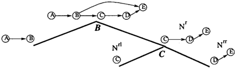
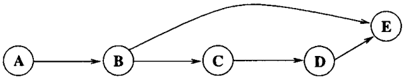
Consider the network N in Figure 1. Figure 2 shows how we can decompose the network into two sub­ networks, N1 and Nr, by instantiating variable B. The figure also shows how we can further decompose network Nr into two subnetworks, Nrl and Nrr, by

instantiating variable C. Note that subnetwork Nr l contains a single node and cannot be decomposed further.

As it turns out, this recursive conditioning process is a special case of a more general phenomenon that applies to any probability distribution which is rep­ resented as the multiplication of factors (h, ... , ¢n. 3

This is the key theorem underlying the more general version of recursive conditioning:

Theorem 1 (Case Analysis) Let ¢ ¢1 q;r , where C are the variables shared by factors ¢1 and q;r, and let X be a subset of the variables over which factor ¢ is defined. Then ¢(x) = Lc ¢1(x1c)¢r(xrc), where x1 and xr are the subsets of instantiation x pertaining to variables in ¢1 and q;r, respectively.

This theorem tells us how to decompose a compu­ tation with respect to a factor ¢ = ¢1¢r into com­ putations with respect to its sub-factors ¢1, q;r by performing a case analysis on the variables shared by these sub-factors. Given a factored represen­ tation ¢ = ¢ 1 , ... , ¢n of a probability distribu­ tion, we can use the theorem recursively to com­ pute ¢(x) as follows. We start by partitioning the factors ¢ 1 , ... , ¢n into two sets, ¢1 = ¢ 1 , ... , ¢ m and q;r = ¢m+ 1, . . . , ¢n, and then apply Theorem 1. We can repeat this process recursively until we hit boundary conditions where we try to compute the probability of some instantiation with respect to a single factor ¢i.

The key to the efficiency of this algorithm is the way we partition a set of factors into two sets ¢1 and q;r. Note that the complexity of the algorithm is expo­ nential in the number of variables shared between factors ¢1 and q;r. We will address the question of generating efficient partitions, but we must first in­ troduce a formal tool for representing a recursive partitioning ( decomposition ) of a set of factors.

3 A factor for variables X, also known as a potential, is a function which maps instantiations x of variables X into numbers cf>(x).

Definition 1 A dtree for a set of factors (!>I, . . . , <Pn is a full binary tree, the leaves of which correspond to the factors ¢1, ... , <Pn. The factor associated with leaf T will be denoted by FACTOR(T).

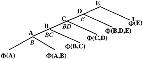
Figure 3 depicts a dtree for the CPTs of the Bayesian network in Figure 1, where each CPT is viewed as a factor. Following standard conventions on binary trees, we will often not distinguish between a node and the dtree rooted at that node. We also use T1' rr' TP to denote the left child, right child, and parent of node T, respectively.

A dtree T suggests that we decompose its associ­ ated factors into those associated with its left sub­ tree T1 and those associated with its right subtree Tr. For example, in Figure 3, we would have ¢ 1 = ¢(A)¢( A, B) and ¢ r = ¢(B, C)¢(C, D)¢(B, D, E). Applying Theorem 1 with x =a, e and C = B, we get ¢(a, e ) = 'f:.b ¢ 1( a b ) ¢ r( eb ) since x 1 = a, xr = e and B is the only variable shared by the left and right subtrees of the dtree.

The variables shared by the left and right subtrees of dtree T, denoted by vars(T1) nvars(Tr), are called the cutset of node T. In Figure 3, B is the cutset of the root node. Each dtree defines a number of cutsets, each associated with one of its nodes.

Definition 2 [3] The cutset of internal node T in a dtree is cutset(T) d.2 vars(T1) n vars(Tr) acutset(T), where acutset(T) is the union of cutsets associated with ancestors of node T in the dtree.

For the root T of a dtree, cutset(T) is simply vars(T1) n vars(Tr). But for a non-root node T, the cutsets associated with ancestors of T are excluded from vars(T1) n vars(Tr) since such cutsets are guar­ anteed to be instantiated when we are about to de­ compose factors under node T.

Given a probability distribution ¢ which is decom­ posed into factors ¢1 . . . <Pn = ¢, and given a dtree T for the factors ¢1, . . . , ¢ n , we can compute the prob­ ability, ¢(e), of any instantiation e with respect to distribution ¢ as follows:

This is clearly a linear-space algorithm. Moreover, the number of recursive calls it makes to any node T is acutset(T)#, where X# is the number of instanti­ ations of variables X. We showed in [3] that given an elimination order of length n and width w, we can generate a dtree in which the size of every a-cutset is O(w logn ) . Using such a dtree, the complexity of RC is O ( nexp ( wlogn ) ) , which is a new complexity result for linear-space probabilistic inference.

A close examination of the above version of RC reveals that it will pose the same query with re­ spect to a subdtree T many times, therefore, per­ forming many redundant computations. Specifically, RC(T, el) = RC(T, e2) whenever e1 and e2 agree on the instantiation of variables appearing in dtree T. The variables in dtree T which are guaranteed to appear in the instantiation e of RC(T, e) are defined as follows:

Definition 3 {3] The context of node T in a dtree is: context(T) d � vars(T) n acutset(T).

Therefore, we can avoid the redundancy by associ­ ating a cache, cacher, with each internal node T in the dtree to save solutions of calls to node T, indexed by the instantiation of context(T) at the time of the call. Each time RC is called on T, it checks the cache ofT first and recurses only if no corresponding cache entry is found. This refined version of recursive con­ ditioning is shown in Figure 4. In this code, we do not pass instantiations as arguments to RC as that is not very efficient. Instead, we record / un-record such instantiations on their corresponding variables. Before the first call to RC is made, the instantia­ tion e is recorded. Each time RC performs a case analysis on variables C, it records the instantiation c under consideration and then un-records it later. The word "possible " on line 06 means "uncontra­ dicted by currently recorded instantiations. " This can be achieved efficiently by enumerating the in­ stantiations of cutset(T) \ E where E are the cur­ rently instantiated variables.

Note also that on line 10, we have included the test cache?(T, y) to control what solutions are cached. As we shall see later, if we cache all solutions (cache?(T, y) succeeds for all T and y), we get the same time and space complexity of elimination and clustering algorithms. The any-space behavior of re-

Algorithm RC RC(T) 01. if Tis a leaf node, 02. then x +---recorded instantiation of vars(T) return FACTOR(T)(x) 03. else y +---recorded instantiation of context(T) 04. if cacher[y] i= nil, return cacher[Y] 05. else p +---0 06. for each possible instantiation c of cutset(T) 07. record instantiation c 08. p +---p + Rc(T1)Rc(Tr) 09. un-record instantiation c 10. when cache?(T, y), cacher[Y] +---p 11. return p

cursive conditioning is due to the fact that we can cache as many solutions as we wish by controlling how the cache?(T, y) test is realized. One sugges­ tion for realizing this test is to use the notion of a cache factor, which controls the size of each partic­ ular cache in a dtree:

Definition 4 [3} A cache factor for a dtree is a function cf that maps each internal node T in the dtree into a number, cf(T), between 0 and 1.

The intention here is for cf(T) to be the fraction of cacher which will be filled by algorithm RC. That is, if cf(T) = .2, then we will only use 20% of the total storage required by cachey. If cf(T) = 0 for every node T, we obtain the linear-space version of RC. Moreover, if cf(T) = 1 for each node T, we obtain another extreme which has the same time and space complexity of clustering and elimination algorithms [3]. The question now is: What can we say about the number of recursive calls made by RC under a par­ ticular cache factor cf? As it turns out, the number of recursive calls made by RC will depend on the par­ ticular instantiations of context(T) that are cached on line 10. However, if we assume that any given instantiation y of context(T) is equally likely to be cached, then we can compute the average number of recursive calls made by RC and, hence, its average running time.4

Theorem 2 [3} If the size of cacher is limited to cf(T) of its full size, and if each instantiation of context(T) is equally likely to be cached on line 10 of RC , the average number of calls made to a non-root

4Note that we can enforce the assumption that any given instantiation y of context(T) is equally likely to be cached by randomly choosing the instantiations to be cached.

node T in algorithm RC is ave(T) = cutset(TP)# [ cf(TP)context(TP)# + (1 - cf(TP) )ave(TP) J .

Recall here that TP is the parent of node T in the dtree.

This theorem is quite important practically as it al­ lows one to estimate the running time of RC under any given memory configuration. Using the theo­ rem, one can plot time-space tradeoff curves for com­ putationally demanding networks-we show such curves in [3]. We note that when the cache factor is discrete (cf(T) = 0 or cf(T) = 1 ) , Theorem 2 pro­ vides an exact count of the number of recursive calls made by RC. In fact, under no caching, cf(T) = 0, the number of calls made to each node T is exactly acutset(T)#. And under full caching, cf(T) = 1, the number of calls made to each non-root node T is exactly cutset(TP)#context(TP)#.5 Given an elimi­ nation order of width w, we can always generate a dtree such that acutset(T)# is O(exp(w log n)), or such that cutset(T)#context(T)# is O(exp(w ) ) [3].

The cluster of node T in a dtree is defined as cutset(T)Ucontext(T) if T is non-leaf, and as vars(T) if T is leaf. The width of a dtree is the size of its maximal cluster minus 1. Under full caching, the time and space complexity of recursive conditioning is O ( n exp ( w )) , where n is the number of factors and w is the width of used dtree [3].

The issue of time-space tradeoff has been receiving increased interest in the context of Bayesian net­ work inference, due mostly to the observation that state-of-the-art algorithms tend to give on space first. The key existing proposal for such tradeoff is based on realizing that the space complexity of clustering algorithms is exponential only in the size of separators, which are typically smaller than clus­ ters [5]. Therefore, one can always trade time for space by using a jointree with smaller separators, at the expense of introducing larger clusters [5]. This method, however, can generate very large clusters which can render the time complexity very high. To address this problem, a hybrid algorithm is proposed which uses cutset conditioning to solve each enlarged cluster, where the complexity of this hybrid method can be less than exponential in the size of enlarged clusters [5].

There are two key differences between this proposal and ours. First, the proposal is orthogonal to our notion of a cache factor, as it can be realized during the construction phase of a dtree. That is, we may

5Theorem 2 assumes that we have no evidence recorded on the dtree. This represents the worst case for RC.

decide to construct a dtree with a smaller caches, yet larger cutsets. But once we have committed to a particular dtree, the cache factor can be used to control the time-space tradeoff at a finer level, al­ lowing us to do the time-space tradeoff at increments of X-bytes, where X is the number of bytes needed to cache a floating point number. The second key difference between the proposal of [5] and ours is that when the hybrid algorithm of [5] is run in linear space, it will reduce to cutset conditioning since the whole jointree will be combined into a single cluster. In our proposal, linear space leads to a different time complexity than that of cutset conditioning.

3 Forgetting

We can improve the memory usage of RC by asking the following question: For how long do we need to cache previous computations?

As it turns out, computing the exact number of times that a cached solution will be accessed by RC depends on which particular instantiations y are cached on line 10. Even if we assume that such in­ stantiations are equally likely to be cached, we will only be able to compute the average number of times that a cache entry will be accessed. However, if we assume that the cache factor is discrete that is, for every node T, either cf(T) = 0 or cf(T) = 1 then one can provide an exact count of the number of times that a cache entry will be retrieved. Once RC retrieves the entry that many times, there is no point of caching the entry any longer-it can simply be forgotten!

Theorem 3 Let T1, T2, . .. , Tn be a descending path in a dtree where

Each entry of cachern will then be retrieved

times by algorithm RC. 6

That is, the exact number of times that entries of cachern will be looked up by RC can be determined based on the context of node Tn, the context of its closest ancestor T1 where caching is also taking place, and the cutsets of all nodes in between T1 and

6 Again, we are assuming here that RC is run with no evidence. The theorem can be easily generalized for the case of existing evidence.

Tn. For the special case of full caching (cf(T) = 1 for all T), we have that each entry in cacher will be retrieved exactly (context(TP) - context(T))# -1 times.

We implemented the simple forgetting technique suggested by Theorem 3 and measured the memory requirement of RC under full caching on a number of realistic networks shown in Table 1. 7 In particular, we kept track of the maximum number of cache en­ tries (cells) during the runtime of the algorithm on each of the networks. We also measured the mem­ ory requirements of variable elimination by keeping track of the maximum number of entries (cells ) in active factors at any time. For both algorithms, we used the elimination orders provided with the net­ works in the repository and assumed no evidence (worst case) .

The second and third columns in Table 1 report log 2 of the number of cells in factors and caches, respec­ tively. The fourth column gives the ratio between the number of cells. The fifth and sixth columns report the actual memory used in megabytes. For elimination, we assumed that each factor cell uses eight bytes, while for recursive conditioning, we as­ sumed that each cache cell requires twelve bytes. The extra four bytes are used to store a counter with each cache cell to keep track of the number of times that the cell has been accessed. As is clear from the numbers, recursive conditioning is system­ atically better as far as its space requirements are concerned, with the difference being very significant in some cases. Our implementation of both algo­ rithms in JAVA also suggest that RC is about twice as fast as VE, although we have no explanation of this.

4 Maximum a Posteriori Hypothesis

Our goal in this section is to present a version of re­ cursive conditioning for computing maximum a pos­ teriori hypotheses (MAP). The MAP problem is de­ fined as follows. Given a probability distribution ¢, a set of variables M, which we call MAP variables, and evidence e, we want to compute

That is, we want all ipstantiations m of variables M for which the probability cjJ(m, e) is maximal.

7 The networks are available in the UC Berkeley Repository (http:/ jwww-nt. cs. berkeley. edu/home/nir jpublic­ htmljrepository /index. htm).

Table 1: Comparing space requirements of recursive conditioning and variable elimination on realistic net­ works. cells# is the maximum number of floating point numbers stored at any time during the runtime of the algorithm.

Network	VE cells# (log2)	RC cells# (log2)	VE cells#/ RC cells#		VE memory RC memory (MB) (MB)	VE memory/ RC memory
Water	20.3	14.3	65.8	10.13	0.23	43.9
Mildew	19.1	15.3	13.6	4.27	0.46	9.0
Barley	20.2	18.7	2.8	9.01	4.87	1.8
Diabetes	18.8	17.5	2.5	3.52	2.12	1.7
Pigs	16.1	14.9	2.3	0.53	0.35	1.5
Link	21.1	17.8	9.9	17.24	2.61	6.6
Munin2	16.7	15.3	2.6	0.80	0.46	1.7
Munin3	18.1	14.8	10.1	2.21	0.33	6.8
Munin4	20.1	17.1	7.9	8.42	1.61	5.2

We also want each of these instantiations associated with the probability ¢(m, e).

A special case of MAP is that of computing the most probable explanation ( MPE ) , denoted by mpe<�>(e), which results from taking M to be the set of all variables over which distribution </> is defined. Ex­ tending RC to compute MPE is straightforward: all we have to do is modify it so it returns a set of pairs (i, p), where i is an instantiation of all variables and p is the probability of such instantiation, p = </>(i). This can be done by:

1. modifying line 02 of RC so it returns (y, FACTOR(T)(y)), where y is an instantia­ tion of vars(T), y is consistent with x, and FACTOR(T)(y) is maximal;
2. modifying line 08 so it performs a maximization instead of summation.

The reason why such an extension works is that MPE computations lend themselves to the principle of case analysis in a straightforward way:

Theorem 4 Let 4> = ¢1</>r, where C are the vari­ ables shared by factors ¢1 and </>r. Then mpe¢ (e) = max Uc mpe¢1(e1c) x mpe¢"(erc), where e1 and er are the subsets of evidence e pertaining to variables in ¢1 and <f>r, respectively, and

That is, the max function returns only those pairs (i,p) in S for which the probability p is maximal. And the x function returns the Cartesian product of two sets. Note that in the definition of x, instan­ tiations i and j may have common variables, but are guaranteed to agree on the values of such variables in this case. This follows because x is only applied to the sets mpe¢1 (e1c) and mpe¢" (ere), which instanti­ ations agree on their common variables C.

Unfortunately, the case analysis principle is not di­ rectly applicable to MAP computations. That is, we cannot in general reduce the computation of map¢(M, e) into that of computing map¢(M, ec) for some set of variables C. To see this, consider the fol­ lowing distribution:

A	B	¢(a, b)
true	true	.32
true	false	.28
false	true	.10
false	false	.30

If we take B to be the MAP variable, and e to be the empty evidence, then we have map¢( {B}, e)= {(B=false, .58)}, while we have map¢({B}, A=true) = {(B=true, .32)} and map¢({B}, A=false) = {(B=false, .30)}. Therefore, if we maximize across the two cases, we get B=true as the most probable hypothesis, which is incorrect.

The principle of case analysis, however, applies to MAP in two special cases: If all variables in the conditioning set C are MAP variables, or if all map variables M appear in the evidence e.

Theorem 5 Let 4> = ¢1</>r, where C are the vari­ ables shared by factors ¢1 and </>r. If C s;; M, then map¢(M, e) = max Uc map¢1 (M1, e1c) x map¢" (Mr, er c), where M1 / e1 and Mr / er are the subsets of M/ e pertaining to variables in ¢1 and <f>r, respectively.

Theorem 4 is a special case of Theorem 5 as C s;; M holds trivially when M includes all variables.

Theorem 6 Let 4> = ¢1</>r, where C are the vari­ ables shared by factors ¢1 and </>r. If M s;; E,

then map<I>(M, e) = {(i,p)}, where i is the sub­ set of evidence e pertaining to variables M and p = :Z::::c q}(e1c)(pr(erc), where e1 and er are the sub­ sets of e pertaining to variables in q} and (pr , respec­ tively.

This theorem may not sound interesting since we only have one most probable hypothesis which can be retrieved in constant time by projecting evidence e on variables M. But our interest here is in the probability of such hypothesis, which is needed as this theorem will be invoked when we apply Theo­ rem 5 recursively.

The above theorems suggest that we split case analy­ sis into two phases. In the first phase, we decompose by case analysis on MAP variables only using Theo­ rem 5, until all MAP variables are instantiated. We can then continue the decomposition process by case analysis on non-MAP variables using Theorem 6. Each phase is then guaranteed to be sound.

This two-phase process has implications. First, we cannot use an arbitrary dtree to drive the decom­ position process, but must use dtrees that satisfy some additional properties. In particular, a cut­ set containing a MAP variable cannot be a descen­ dant of a cutset containing a non-MAP variable. Second, this means that computing MAP is harder than computing marginals or MPE, since it reduces the space of legitimate dtrees, possibly ruling out the optimal dtrees (ones with smallest width) from consideration. 8

We show in the following section how to induce dtrees that have such a property. In particular, given an elimination order 1r in which non-MAP variables are eliminated before MAP variables, we show how to induce a dtree T based on 1r such that: the width ofT is no greater than the width of 1r; and no MAP cutset is a descendant of a non-MAP cutset. This means that the time and space complexity of our al­ gorithm (under full caching) will be O(nexp(w))­ where n is the number of factors, and w is the width of given elimination order therefore, matching the complexity of elimination algorithms for MAP [4]. The win, however, is that our algorithm ex­ hibits smooth any-space behavior. Moreover, it is equipped with a formula for predicting its running time under any amount of memory, which allows us to construct smooth time-space tradeoff curves for computationally demanding networks.

Figure 5 provides the pseudocode for algorithm RC-

8 This phenomenon is also true in variable elimination algorithms for computing MAP, so it appears to be a property of MAP rather than a problem of our approach for computing it [4].

Algorithm RC-MAP RC-MAP(T) 01. if Tis a leaf node, 02. then return LOOKUP(T) 03. else y +-recorded instantiation of context(T) 04. if cacher[y] =/= nil, return cacher[Y] 05. else if MAP-NODE?(T) 06. then S +-RC-MAX(T) 07. else S +-RC-SUM(T) 08. when cache?(T, y), cacher[Y] +-S 09. return S LOOKUP(T) 01. f +-recorded instantiation of variables in FACTOR(T) 02. f' +-subset of f corresponding to MAP variables 03. return {(f', FACTOR(T)(f))}

MAP. As we shall see in the following section, the dtrees we shall generate have two additional proper­ ties which simplify the statement of RC-MAP: each cutset is either empty or a singleton; and each vari­ able appears in some cutset. When the cutset of node T contains a MAP variable, the test MAP­ NODE?(T) on line 05 succeeds.

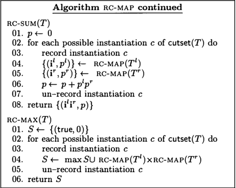
RC-MAP has the same structure as RC aside from a few exceptions. First, it returns a set of pairs (i,p), where i is an instantiation and p is a proba­ bility. Second, each time a leaf node T is reached, all variables appearing in the factor FACTOR(T) are guaranteed to be instantiated. Third, RC-MAP will either perform a summation or a maximization at each node, depending on whether the node cutset contains a MAP variable. The summation and max­ imization code are shown in Figure 6.

One observation about RC-SUM in Figure 6 is that each time RC-SUM is called on a node T, all MAP variables appearing under T are guaranteed to be instantiated. Therefore, in the case analysis per­ formed by RC-SUM, the instantiations i1ir returned by each of the cases is the same. Moreover, RC-SUM will always return a singleton, which explains the as­ signments on lines 04 and 05. We assume here that the number of maximum a posteriori hypotheses is small enough to be considered a constant. If this is not the case, we can easily modify RC-MAP so it only returns a single hypothesis by changing the def­ inition of max so it returns a single maximum pair instead of all such pairs.

We close this section by pointing out an impor­ tant difference between RC-MAP and similar algo­ rithms based on variable elimination. Specifically, suppose that we have called RC-MAP(T) after having

Algorithm RC-MAP continued
RC-SUM(T)
01.	p +- 0
02.	for each possible instantiation c of cutset(T) do
03.	record instantiation c
04.	{(i1,p1)} +- RC-MAP(T1)
05.	{(ir, pr)} +- RC-MAP(Tr)
06.	p +- p + p l pr
07.	un-record instantiation c
08.	return {(i1ir,p)}
RC-MAX(T)
01.	S +- {(true, 0)}
02.	for each possible instantiation c of cutset(T) do
03.	record instantiation c
04.	S +- maxSU RC-MAP(T1)XRC-MAP(Tr)
05.	un-record instantiation c
06.	return S

recorded evidence e. Suppose further that we want to compute MAP for a new evidence e ' . One way to do this is to start a brand new computation with respect to T. That is, we remove evidence e, initial­ ize all caches, record evidence e ' and then call RC­ MAP ( T ) again. This is actually an overkill! Specifi­ cally, if the evidence on some factor FACTOR ( T ) has changed, then all we need to do is initialize caches that are associated with ancestors of leaf node T. This means that the second call to RC-MAP will reuse some of the computations performed with respect to the first call. As it turns out, this may lead to sig­ nificant savings in certain cases. Table 2 depicts the results of an experiment illustrating this sav­ ing. For some of the networks in Table 1 (ones with small width), we declared the last five variables in the associated elimination orders as MAP variables. We then computed MAP assuming no evidence and recorded the number of recursive calls made by Re­ MAP (assuming full caching). We then iterated on each of the variables in the network, declaring ev­ idence on the variable, recomputing MAP as de­ scribed above, and then removing the declared ev­ idence. We recorded the number of recursive calls made by RC-MAP in each case, divided by the num­ ber of calls it made in the very first query, and then reported the statistics in Table 2. As is clear from this table, the average number of recursive calls in subsequent queries is much reduced in certain cases due to computation reuse, going as low as 1% in certain cases.

Table 2: The average is over all variables for first three networks, and over 50 random variables for rest. ave: stands for average and std: stands for standard deviation.

Network	No. Calls in subsequent query/ No. Calls in first query ave% std% min% max%
Water	51	25	6	98
Mildew	40	21	1	81
Barley	77	32	8	94
Pigs	59	30	1	91
Munin2	17	6	9	26

5 From Elimination Orders to Dtrees

Let <Pl , ... , <Pn be a set of factors and let 1r be an elimination order used to drive variable elimination on these factors. We present in this section a linear­ time algorithm for converting order 1r into a dtree such that:

1. The width of dtree is no greater than the width of 1r.
2. Every variable of 1r appears in some dtree cut­ set.
3. Each cutset is either empty or a singleton.
4. X E cutset(Tx ), Y E cutset(Ty ), and Tx is a descendant of Ty only if X appears before Y m 1f.

Such a dtree is needed for the correctness of algo­ rithm RC-MAP which we presented in the previous section. Property 4 is most important as it implies that by the time we start doing a case analysis on a non-MAP variable in cutset(T), all MAP variables appearing in the factors of T are guaranteed to have been instantiated.

We have presented in [3] a linear-time algorithm, EL2DT, for converting an elimination order 1r into a dtree T, with the guarantee that the width ofT is no greater than the width of 1r. Interestingly enough, we can modify this algorithm slightly to obtain the extra properties we listed above. We will first ex­ plain EL2DT and then present the mentioned modi­ fication.

Given factors ¢1, ... , ¢n, EL2DT works by first con­ structing a dtree LEAF( ¢i) consisting of a single node for each factor <Pi. It then considers variables accord­ ing to given order 1r. When variable X is considered, EL2DT collects all dtrees which mention X and con­ nects them, arbitrarily, into a binary tree. When all variables have been considered, EL2DT connects all remaining dtrees into a binary tree and returns

Figure 7: Pseudocode for transforming an elimina­ tion order into a dtree. LEAF( ifJ) creates a leaf node and associates factor ifJ with it. COMPOSE(I:) con­ nects the dtrees in I: into a binary tree.

Algorithm EL2SDT
I* e is a set of factors *1 1* 1r an elimination order of variables in e *1 EL2SDT(8, 1r ) 01. I: f- {LEAF( <f>) : <f> is a factor in E)} 02. for i f- 1 to length of order 1r do 03. let r be trees in I: which contain variable 7r(i) 04. if r is a singleton, r f- r U {LEAF(<f>1( 1r ( i)))} os. I: f- I: \ r 06. I: f- I: U {COMPOSE(r)} 07. return COMPOSE(I:)

the result. The pseudocode of EL2DT is exactly as given in Figure 7, except for line 04 which has been added to obtain the additional properties needed by RC-MAP.

Specifically, when variable X is considered by EL2DT, it is possible that only one dtree Tx will mention X. EL2DT will do nothing in this case. But algorithm EL2SDT in Figure 7 will perform an extra step:

• -it will introduce a unit factor ¢1 over variable X, that is, ¢1(x) = 1 for all x; and
• -it will construct a single node dtree, LEAF(¢1 ) , for the unit factor ¢1 ;

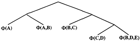
therefore, causing dtrees Tx and LEAF(¢1) to be con­ nected together. Note that in doing so, EL2SDT is adding additional factors to the initial set of factors, but that affects neither soundness nor complexity. Figure 8 depicts an example where a dtree is con­ structed for the network in Figure 1, using the elim­ ination order 7r =<A, B, C, D, E >.

Theorem 7 If we construct a dtree based on elimi­ nation order 1r using EL2SDT, then it will satisfy the four properties listed earlier in the section.

We close this section by noting that algorithm EL2SDT is important not only for computing MAP, but for inference in conditional Gaussian networks which contain both discrete and continuous variables [2]. In such networks, we must also eliminate all con­ tinuous variables first, therefore, requiring special dtrees such as those constructed by EL2SDT. We are currently working on an extension of recursive conditioning for dealing with such networks.

6 Conclusion

This paper rests on several contributions. First, a generalization (and simplification) of the any-space recursive conditioning algorithm so it applies to any factored representation of probability distributions. Second, a solution-forgetting technique which re­ duces the space constant factors of recursive con­ ditioning to the point where it becomes orders of magnitude more space efficient than variable elimi­ nation on some realistic networks. Third, the first MAP algorithm allowing a smooth tradeoff between time and space, which is also equipped with a for­ mula for predicting its running time under any space configuration. Finally, two key theorems shedding some light on the use of case analysis in MPE and MAP computations.

References

• [ 1 ] Gregory F. Cooper. Bayesian belief-network in­ ference using recursive decomposition. Tech­ nical Report KSL-90-05, Knowledge Systems Laboratory, Stanford, CA 94305, 1990.
• R. Cowell, A. Dawid, S. Lauritzen, and D. Spiegelhalter. Probabilistic Networks and Expert Systems. Springer, 1999.
• [ 3 ] Adnan Darwiche. Recursive conditioning: Any­ space conditioning algorithm with treewidth­ bounded complexity. Artificial Intelligence Journal, 2000. To appear in special issue on resource bounded reasoning.
• [ 4 ] Rina Dechter. Bucket elimination: A unifying framework for probabilistic inference. In Pro­ ceedings of the 12th Conference on Uncertainty in Artificial Intelligence (UAI), pages 211-219, 1996.
• Rina Dechter. Topological parameters for time­ space tradeoff. In Proceedings of the 12th Con-

ference on Uncertainty in Artificial Intelligence (UAI), pages 211-219, 1996.

1. Cecil Huang and Adnan Darwiche. Inference in belief networks: A procedural guide. In­ ternational Journal of Approximate Reasoning, 15(3) :225-263, 1996.
2. F. V. Jensen, S.L. Lauritzen, and K.G. Olesen. Bayesian updating in recursive graphical mod­ els by local computation. Computational Statis­ tics Quarterly, 4:269-282, 1990.
3. Judea Pearl. Probabilistic Reasoning in Intelli­ gent Systems: Networks of Plausible Inference. Morgan Kaufmann Publishers, Inc., San Mateo, California, 1988.
4. Mark A. Peot and Ross D. Shachter. Fusion and propagation with multiple observations in belief networks. Artificial Intelligence, 48(3):299-318, 1991.
5. R. Shachter, B.D. D'Ambrosio, and B. del Favero. Symbolic Probabilistic Inference in Be­ lief Networks. In Proc. Conf. on Uncertainty in AI, pages 126-131, 1990.
6. Nevin Lianwen Zhang and David Poole. Ex­ ploiting causal independence in bayesian net­ work inference. Journal of Artificial Intelligence Research, 5:301-328, 1996.