一

Approximating MAP using Local Search

James D. Park and Adnan Darwiche

Computer Science Department University of California Los Angeles, CA 90095 {jd,darwiche }@cs.ucla.edu

Abstract

MAP is the problem of finding a most prob­ able instantiation of a set of variables in a Bayesian network, given (partial) evidence about the complement of that set. Unlike computing priors, posteriors, and MPE (a special case of MAP), the time and space complexity of MAP is not only exponen­ tial in the network treewidth, but also in a larger parameter known as the "constrained" treewidth. In practice, this means that com­ puting MAP can be orders of magnitude more expensive than computing priors, pos­ teriors or MPE. For this reason, MAP com­ putations are generally avoided or approxi­ mated by practitioners.

One specialization of MAP, which has received a lot of attention, is the Most Probable Explanation (MPE) [15]. MPE is the problem of finding the most likely configuration of a set of variables given a partic­ ular instantiation of the complement of that set. The primary reason for this attention to MPE is that it seems to be a much simpler problem than its MAP generalization.

We have investigated the approximation of MAP using local search. The local search method has a space complexity which is ex­ ponential only in the network treewidth, as is the complexity of each step in the search process. Our experimental results show that local search provides a very good approxima­ tion of MAP, while requiring a small number of search steps. Practically, this means that the average case complexity of local search is often exponential only in treewidth as op­ posed to the constrained treewidth, mak­ ing approximating MAP as efficient as other computations.

1 Introduction

The task of computing the Maximum a Posterior hy­ pothesis (MAP) is to find the most likely configuration of a set of variables (which we call the MAP variables) given (partial) evidence about the complement of that set (the non-MAP variables).

Unfortunately, MPE is not always suitable for the task at hand. For example, in system diagnosis, where the health of each component is represented using a vari­ able, one is interested in finding the most likely config­ uration of health variables only-the likely input and output values for each component are not of interest. Additionally, the projection of an MPE solution on these health variables is not necessarily a most likely configuration. Nor is the configuration which results from choosing the most likely state of each variable separately.

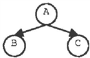
Computing MAP seems to be significantly more diffi­ cult than computing priors, posteriors or MPE. All of these problems are NP-Hard, including their approxi­ mations [1, 3], but the computational resources needed to solve MAP using state-of-the-art algorithms are much greater than those needed to compute MPE, for example. Suppose that we decide to solve MAP and MPE using a variable elimination algorithm [16, 8]. Although we can use any elimination order to com­ pute MPE, we can only use a subset of these orders to compute MAP. Specifically, for an elimination algo­ rithm to be sound for MAP, it requires that we elim­ inate the non-MAP variables first. This reduces the space of elimination orders, possibly throwing out the most efficient orders from consideration. As an exam­ ple, consider the network in Figure 1, which admits 6 different elimination orders. Any of these orders can be used to solve MPE. To compute MAP of variables B,C, however, only two of these orders can be used and the width of each is 2. Note that we could use an order of width 1 for computing MPE in this case.

Figure 1: A simple network, its possible elimination orders, the widths, and whether or not each order can be used for MPE, and MAP(B,C). Requiring that A be eliminated before B and C forces the width of the elimination order used for MAP(B,C) to be 2, while an order of width 1 can be used for MPE.

Order	Width	MPE Order	MAP Order
ABC	2	X	X
ACB	2	X	X
BAC	1	X
BCA	1	X
CAB	1	X
CBA	1	X

The complexity of a variable elimination algorithm is exponential in the (induced) width of the used elimina­ tion order .1 Hence, the increase in such a width when computing MAP can be critical: it may simply make a particular network inaccessible to variable elimination algorithms when computing MAP, even though it is accessible when computing MPE.

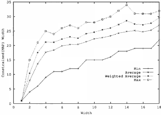
In order to assess the magnitude of increase in width caused by restricting elimination orders, we gener­ ated 1000 Bayesian networks randomly as given in Appendix A and then computed the constrained and unconstrained elimination orders for these networks using the min-fill heuristic [12, 9). For constrained orders, all non-MAP variables were eliminated first. Each network had 100 nodes and the set of MAP vari­ ables consisted of 10-25 root nodes. We measured the minimum, maximum, average and weighted average width for the two classes of orders.The average was computed as 2:�1 wifk. Since the complexity is ex­ ponential in the width, a weighted sum gives a better representation of the average complexity. It was com­ puted as log2(2:�=1 2w· /k). Figure 2 summarizes the results.

In many cases, the constrained width was much larger than the unconstrained width, often making the MAP problem unreasonably expensive, even when the MPE problem could be solved exactly with reasonable re­ sources. For example, the weighted average width in-

1The width of an elimination order with respect to a network is defined as the size of the maximal clique -1 in a jointree constructed based on the elimination order. It can also be equivalently defined as the number of variables -1 in the largest table constructed when running variable elimination using the order.

creased from about 13 to about about 27 due to MAP constraints. That is, even though the largest table con­ structed by variable elimination has about 214 entries when computing MPE, the algorithm needs to con­ struct a table with about 228 entries when computing MAP.

The additional resources needed to solve MAP are not only a property of variable elimination algorithms, but are also shared by other algorithms, such as clustering [13, 10, 9] and conditioning [4]. There is definitely a gap between our ability to solve MAP and MPE prob-­ lems, which is best witnessed by the lack of support for MAP algorithms in existing commercial tools for Bayesian network inference.

In this paper, we propose and investigate a method for approximating MAP using local search. The lo­ cal search method has a space complexity which is exponential only in the network treewidth, as is the complexity of each step in the search process. Our experimental results show that local search provides a very good approximation of MAP, while requiring a small number of search steps. Practically, this means that the average case complexity of local search is of­ ten exponential only in treewidth as opposed to the constrained treewidth, making MAP computations as efficient as other computations.2

2 Approximating MAP using Local Search

Given a Bayesian network B which induces a proba­ bility distribution Pr, and given a set of MAP vari­ ables S, the goal of a MAP algorithm is to compute an instantiations that maximizes Pr(s I e) for some evidence e.3

Since computing MAP is often intractable, approxima­ tion techniques are needed. A common approximation technique is to compute an MPE and then project the result on the MAP variables. That is, if S' is the complement of variables S U E, we compute an in­ stantiation s,s ' that maximizes Pr(s,s' I e) and then return s. Another approximation is to compute pos­ terior marginals for MAP variables, Pr(S I e), S E S, and then choose the most likely state s of each vari-

2The network treewidth is defined as the width of its best elimination order. The constrained treewidth is de­ fined as the width of its best constrained elimination or­ ders; hence, is defined with respect to a set of MAP variables.

3We are using the standard notation: variables are de­ noted by upper-case letters (A) and their values by lower­ case letters ( a ) . Sets of variables are denoted by bold-face upper-case letters {A) and their instantiations are denoted by bold-face lower-case letters (a).

30 35 .----.---�

0 0 �--�----L---�---�

able given e. In [7] genetic algoritms were applied to approximate the best k configurations of the MAP variables (this problem is known as partial abduction). We investigate in this paper a different approximation technique based on local search, which works as fol­ lows:

1. Start from an initial guess s at the solution.
2. Iteratively try to improve the solution by moving to a better neighbors': Pr( s ' I e) > Pr(s I e), or equivalently Pr(s', e) > Pr(s, e).

A neighbor of instantiation s is defined as an instanti­ ation which results from changing the value of a single variable X in s. If the new value of X is x, we will denote the resulting neighbor by s - X, x. In order to perform local search efficiently, we need to compute the scores for all of the neighbors s - X, x efficiently. That is, we need to compute Pr(sX, x, e) for each X E S and each of its values x not in s. If variables have binary values, we will have I S I neighbors in this case.

Local search has been proposed as a method for ap­ proximating MPE [11, 14]. For MPE, the MAP vari­ ables S contain all variables which are not in E (the evidence variables). Therefore, the score of a neighbor, Pr(s-X,x, e), can be computed easily since s-X, x, e is a complete instantiation. In fact, given that we have computed Pr(s, e), the score Pr(s -X, x, e) can be computed in constant time.4

4 This assumes that none of entries in the CPTs are 0.

Unlike MPE, computing the score of a neighbor, Pr(s-X,x,e), in MAP requires a global computation since s -X, x, e may not be a complete instantiation. One of the main observations underlying our approach, however, is that the score Pr(s-X,x,e) can be com­ puted in O(nexp(w)) time and space where n is the number of network variables and w is the width of a given elimination order (we can use any elimination order for this purpose, no need for any constraints). In fact, we can even do better than this by computing the scores of all neighbors Pr ( s - X, x, e) (that is, for all X E Sand every value x of X) in O(n exp(w)) time and space. There are a couple of ways to do this. We can use a modification of the technique of fast retrac­ tion in jointrees, which requires working with a special kind of a jointree [2]. An alternative, more direct ap­ proach is to use differential inference [5].

According to this approach, the probability distribu­ tion of a Bayesian network can be represented as a multivariate polynomial P(J..:rn .. . ), in which we have a variable Az for each value x of each network vari­ able. Variables Az are called evidence indicators as we can use them to capture evidence: The probabil-

If there are 0 entries in the CPTs, it may take time linear in the number of network variables to compute the score. Pr{s, e) is the product of the single entry of each CPT that is compatible with s, e. When changing the state of variable X from x to x', the only values in the product that change are those from the CPTs of X and its children. If none of the CPT entries are 0, Pr(s- X,x',e) can be computed by dividing Pr(s, e) by the old and multiplying by the new entry for the CPTs for X and its children. This can be done in constant time if the number of children is bounded by a constant.

ity of some evidence e can be obtained by evaluating the polynomial P while setting each indicator Ax to 1 if x is consistent with e and to 0 otherwise. The value of the polynomial under these indicator settings is denoted by P(e). As is shown in [5]:

Moreover, we can compute the above partial deriva­ tives for all Aa: in only O(nexp(w)) time and space.5 This means that if we have an elimination order of width w for the given Bayesian network, then we can perform each search step in O(nexp(w)) time and space. As we shall see later, it takes a small num­ ber of search steps to obtain a good MAP solution. Hence, the overall runtime is often O(nexp(w)) too. Therefore, we can solve MAP in time and space which are exponential in the unconstrained width instead of the constrained one, which is typically much larger.

The local search method proposed in this section dif­ fers from the local search methods used for MPE in that the unconstrained width must be small enough so that a search step can be performed relatively effi­ ciently. It is pointless to use this method to approx­ imate MPE since in the time to take one step, the MPE could be computed exactly. This method is ap­ plicable when the unconstrained width is reasonable but the constrained width is not (see Figure 2).

3 Description of the Methods Used

3.1 Search Methods

We tested two common local search methods, hill climbing with random restart and taboo search. They differ mainly in how they proceed once a peak (local maximum) is reached.

Hill climbing with random restart proceeds by repeat­ edly changing the the state of the variable that cre-

�The view of a network distribution as a multivariate polynomial P(..\.,, .. . ) is what motivated our investigation of local search methods. Specifically, the probability of instantiation 8 corresponds to the value of polynomial P under a particular indicators setting (,\., = 1 if x is con­ sistent with 8 and >.., = 0 otherwise.) This allows us to view the computation of MAP as an optimization problem where we are looking for the values of indicators >.., (in­ stantiation 8 ) that maximize the value of polynomial P. A natural way for addressing this problem is to use gradi­ ent descent search, especially that computing the gradient 8Pf8..\., can be done efficiently. Interestingly enough, the derivative 8P(s)f8>.., is nothing but the probability of cur­ rent instantiation 8 after having changed a single variable X to x, Pr(8X, x). Our initial approach was to imple­ ment a standard gradient descent method, where we take a small step in the direction of the gradient. But we then realized that the presented (simpler) approach works quite well, so we opted for it instead.

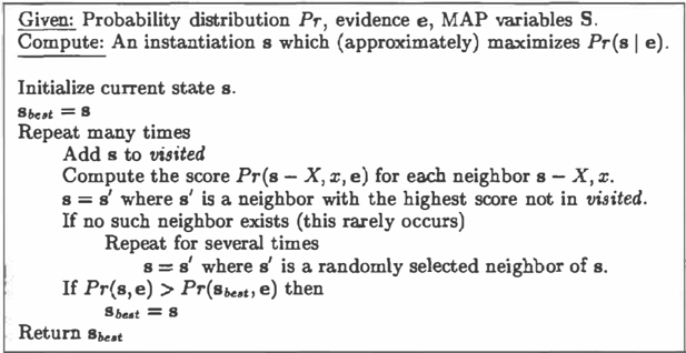
ates the maximum probability change. When a peak is reached, a series of random moves are taken to get to a new start location. Figure 3 gives the algorithm explicitly.

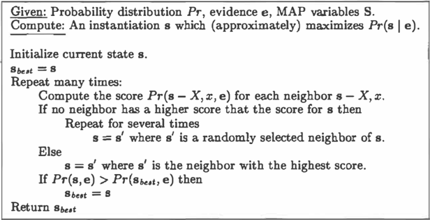
Another variant of hill climbing we implemented is taboo search. Taboo search is similar to hill climb­ ing except that the next state is chosen as the best state that hasn't been visited recently. Because the number of iterations is relatively small we save all of the previous states so that at each iteration a unique point is chosen. Pseudocode for taboo search appears in Figure 4.

3.2 Initialization

The quality of the solution returned by a local search routine depends to a large extent on which part of the search space it is given to explore. We imple­ mented several algorithms to compare the solution quality with different initialization schemes. Suppose that n is the number of network variables, w is the width of a given elimination order, and m is the num­ ber of MAP variables.

1. Random initialization (Rand). For each MAP variable, we select a value uniformly from its set of states. This method takes O(m) time.
2. MPE based initialization (MPE). We compute the MPE solution given the evidence. Then, for each MAP variable, we set its value to the value that the variable takes on in the MPE solution. This method takes O(nexp(w)) time.
3. Maximum likelihood initialization (ML). For each MAP variable X, we set its value to the instance x that maximizes P r ( x I e ) . This method takes O(nexp(w)) time.
4. Seq1.1ential intialization (Seq). This method con­ siders the MAP variables X1. ... , Xm, choosing each time a variable xi that has the highest prob­ ability Pr(xi I e, y) for one of its values Xi, where y is the instantiation of MAP variables considered so far. This method takes O(mn exp(w)) time.

4 Experimental Results

Two search methods (Hill and Taboo) and. four ini­ tialization methods (Rand, MPE, ML, Seq) lead to 8 possible algorithms. Each of the initialization meth­ ods can also be viewed as an approximation algorithm since one can simply return the computed initializa­ tion. This leads to a total of 12 different algorithms. We experimentally evaluated and compared 11 of these

·

一

algorithms, leaving out the algorithm corresponding to random initialization.

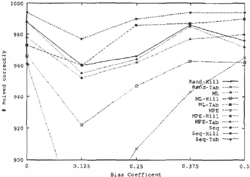
To test the quality of various algorithms, we gener­ ated random network structures using two generation methods (see Appendix A). For each structure, we quantified the CPTs for different bias coefficients from 0 (deterministic except the roots), to .5 (values cho­ sen uniformly) so we could evaluate the influence of CPT quantification on the solution quality. Each net­ work consisted of 100 variables, with some of the root variables chosen as the MAP variables. If there were more than 25 root variables, we randomly selected 25 of them for the MAP variables. Otherwise we used all of the root variables. We chose root nodes for MAP variables because typically some subset of the root nodes are the variables of interest in diagnostic applications. Evidence was set by iru�tantiating leaf nodes. Care was taken to insure that the instantia­ tion had a non zero probability. Each algorithm was allowed 150 network evaluations.6 We computed the true MAP and compared it to the solutions found by each algorithm. Additionally, we measured the num­ ber of network evaluations needed to find the solution each algorithm subsequently returned, and the num­ ber of peaks discovered before that solution was dis­ covered.

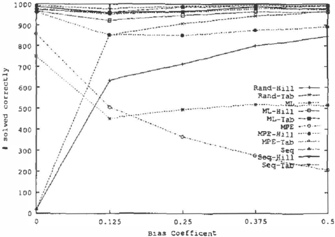
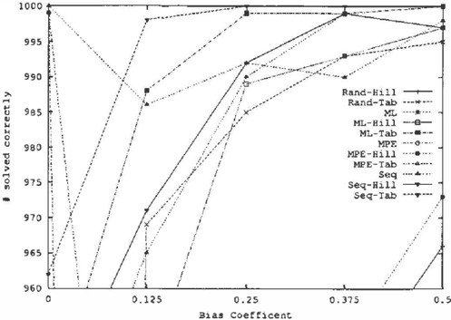
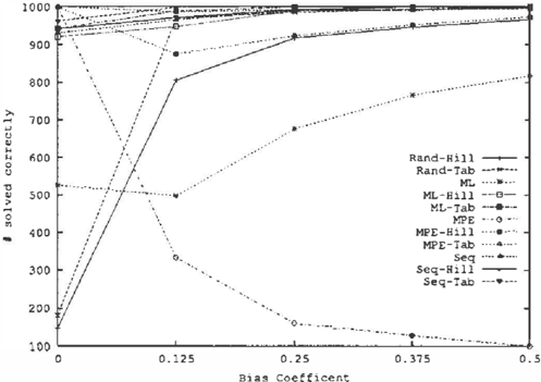
We generated 1000 random network structures for each of the two structural generation methods. For each random structure generated, and each quantification method, we quantified the network, computed the ex­ act MAP, and applied each of the approximation algo­ rithms. Figures 5 and 6 show the solution quality of each of the methods by reporting the fraction of net­ works that were solved correctly; that is, the approxi­ mate answer had the same value as the exact answer.

6 An evaluation takes O(nexp(w)) time and space, where n is the number of network variables and w is the width of given elimination order.

Data Set 1 Solution Quality

	0	.125	.250	.375	.5
Rand-Hill	147	805	917	946	966
Rand-Taboo	181	969	985	993	995
ML	526	497	676	766	817
ML-Hill	920	947	989	993	997
ML-Taboo	942	988	999	999	1000
MPE	999	333	160	127	100
MPE-Hill	999	875	923	952	973
MPE-Taboo	1000	986	992	990	998
Seq	930	965	990	999	997
Seq-Hill	941	971	992	999	997
Seq-Taboo	962	998	1000	1000	1000

Table 1: The solution quality of each method for the first data set. This data is the same as displayed in figure 5. The number associated with each method and bias is the number of instances solved correctly out of 1000. The best scores for each bias are shown in bold.

One can draw a number of observations based on these experiments:

• In each case, taboo search performed slightly bet­ ter than hill climbing with random restarts.
• The search methods were typically able to per­ form much better than the initialization alone.
• Even from a random start, the search methods were able to find the optimal solution in the ma­ jority of the cases.

Data Set 2 Solution Quality

	0	.125	.250	.375	.5
Rand-Hill	20	634	713	799	845
Rand-Taboo	20	851	907	943	965
ML	749	453	495	519	514
ML-Hill	966	922	947	963	962
ML-Taboo	973	960	986	987	990
MPE	858	505	365	275	206
MPE-Hill	961	853	850	874	891
MPE-Taboo	978	952	962	977	980
Seq	988	955	964	985	972
Seq-Hill	988	960	966	986	976
Seq-Taboo	994	977	990	994	994

Table 2: The solution quality of each method for the second data set. This data is the same as displayed in figure 6. The number associated with each method and bias is the number of instances solved correctly out of 1000. The best scores for each bias are shown in bold.

• Overall, taboo search with sequential initializa­ tion performed the best, but required the most network evaluations.

Table 3 contains some statistics on the number of net­ work evaluations (including those used for initializa­ tion) needed to achieve the value that the method fi.:. nally returned. The mean number of evaluations is quite small for all of the methods. Surprisingly, for the hill climbing methods, the maximum is also quite small. In fact, after analyzing the results we discov­ ered that the hill climbing methods never improved

Bias Coefficent

Figure 6: The solution quality of the various search and initialization methods for the second random generation method. The y-axis is the number of problems solved correctly out of 1000. The x-coordinate is the bias coefficient used for quantifying the CPTs. The plot on the right is a zoomed view of the one on the left.

Evaluations Required

Method	Mean	Stdev	Max
Rand Hill	12.5	2.5	21
Rand Taboo	14.3	11.0	144
MPE	1	0	1
MPE Hill	2.6	1.3	8
MPE Taboo	4.0	8 . 3	137
ML	1	0	1
ML Hill	1.6	. 7 4	4
ML Taboo	1.9	3.3	62
Seq	25	0	25
Seq Hill	25.0	.04	26
Seq Taboo	25.0	.9	45

Table 3: Statistics on the number of evaluations each method required before achieving the value it eventu­ ally returned. These are based on the random method 2, bias .5 data set. The statistics for the other data sets are similar.

over the first peak they discovered. 7 This suggests that one viable method for quick approximation is to simply climb to the first peak and return the result. Taboo search on the other hand was able to improve on the first peak in some cases.

7It appears that the random walk used in restarting does not make eventually selecting a better region very likely when using so few search steps. Often, when a sub optimal hill was encountered, the optimal hill was just 2 or 3 moves away. In those cases, the taboo search was usually able to find it (b ecaus e i t s search was more guided), while random walking was not.

5 Discussion

The primary advantage of approximating MAP us­ ing local search in place of solving it exactly using structure-based methods is that local search typically requires much less time and space, yet produces very good approximations. Given a network with n vari­ ables and an elimination order of width w, local search requires O(nexp(w)) space. Standard exact algo­ rithms require O(nexp(wc)) space, where We is the width of a constrained elimination order. Moreover, the time complexity of local search is O(inexp(w)), where i is the number of search steps. An exact algo­ rithm on the other, would require O(n exp(wc)) time. As our experiments have shown, i can be quite small, while the difference between exp(w) and exp(wc) can be quite significant. Therefore, many MAP problems that are intractable for exact methods can be approx­ imated well and efficiently using local search.

Local search methods also have a big advantage over MPE and ML approximations (the methods typically used in place of MAP in diagnosis) in that it is much more accurate. With just a few (in some of our ex­ periments 2-5) network evaluations, one can use ML or MPE to initialize, and then hill climb to produce a drastically better MAP solution. If more accuracy is desired, sequential initialization can be used with hill climbing or taboo search instead, at a cost of a few more network evaluations.

References

• (11 G. Cooper. Computational complexity of prob­ abilistic inference using Bayesian belief networks

(Research note). SIAM Journal on Computing, 42:393-405, 1990.

1. R. Cowell, A. Dawid, S. Lauritzen, and D. Spiegelhalter. Probabilistic Networks and Ex­ pert Systems. Springer, 1999.
2. Paul Dagum and Michael Luby. Approximating probabilistic inference in bayesian belief networks is NP-hard. Artificial Intelligence, 60:141-153, 1993.
3. Adnan Darwiche. Any-space probabilistic infer­ ence. In 16th Conference on Uncertainty in Arti­ ficial Intelligence, pages 133-142, 2000.
4. Adnan Darwiche. A differential approach to infer­ ence in bayesian networks. In 16th Conference on Uncertainty in Artificial Intelligence, pages 123132, 2000.
5. Adnan Darwiche. Recursive conditioning. Artifi­ cial Intelligence, 126(1-2):5-41, February, 2001.
6. [7} L. de Campos, J. Gamez, and S. Moral. Partial abductive inference in bayesian belief networks using a genetic algorithm. Pattern Recognition Letters, 20(11-13):1211-1217, 1999.
7. Rina Dechter. Bucket elimination: A unifying framework for probabilistic inference. In 12th Conference on Uncertainty in Artificial Intelli­ gence, pages 211-219, 1996.
8. Cecil Huang and Adnan Darwiche. Inference in belief networks: A procedural guide. In­ ternational Journal of Approximate Reasoning, 15(3):225-263, 1996.
9. F. V. Jensen, S.L. Lauritzen, and K.G. Olesen. Bayesian updating in recursive graphical models by local computation. Computational Statistics Quarterly, 4:269-282, 1990.
10. [ 1 1] K. Kask and Rina Dechter. Stochastic local search for bayesian networks. In Seventh International Workshop on Artificial Intelligence, Fort Laud­ erdale, FL, 1999. Morgan Kaufmaann.
11. U. Kjaerulff. Triangulation of graphs-algorithms giving small total state space. Technical Report R-90-09, Department of Mathematics and Com­ puter Science, University of Aalborg, Denmark, 1990.
12. S. L. Lauritzen and D. J. Spiegelhalter. Lo­ cal computations with probabilities on graphical structures and their application to expert sys­ tems. Journal of Royal Statistics Society, Series B, 50(2):157-224, 1988.
13. 0. J. Mengshoel, D. Roth, and D. C. Wilkins. Stochastic greedy search: Efficiently computing a most probable explanation in bayesian networks. Technical Report UIUCDS-R-2000-2150, U of Illi­ nois Urbana-Champaign, 2000.
14. Judea Pearl. Probabalistic Reasoning In Intelli­ gent Systems. Morgan Kaufmann, 1998.
15. Nevin Lianwen Zhang and David Poole. Ex­ ploiting causal independence in bayesian network inference. Journal of Artificial Intelligence Re­ search, 5:301-328, 1996.

A Generating Random Networks

We generated several types of networks to perform our experiments. We used two methods for generating the structure, and a single parametric method for gener­ ating the quantification.

A.l Generating the Network Structure

The first method is parameterized by the number of variables N and the connectivity c. This method tends to produce structures with widths that are close to c. See [6J for an algorithmic description.

The second method is parameterized by the number of variables N, and the probability p of an edge being present. We generate an ordered list of N variables, and add an edge between variables X and Y with prob­ ability p. The edges added are directed toward the variable that appears later in the order.

For the experiment in Figure 2, we used method 1 with N = 100 and c between 1 and 20.

For the experiments in Figures 5 and 6, we used N = 100, c between 6 and 12, and p = .025. These numbers were chosen so that the MAP width would be small enough that we could compute the exact value to measure the solution quality.

A.2 Quantifying the Dependencies

The quantification method is parameterized by a bias parameter b. The values of the CPTs for the roots were chosen uniformly. The values for the rest of the nodes were based on a bias, where one of the values v was chosen uniformly in [0, b), and the other as 1v. For example, for b = .1, each non root variable given its parents has one value in [0, .1), and the other in (.9, 1]. Special cases b = 0, and b = .5 produce determistic, and uniformly random quantifications respectively.