Contents
1301.2313
Bayesian Error-Bars for Belief Net Inference
Tim Van Allen digiMine, Inc. 10500 NE 8th St. Floor 13 Bellevue, WA 98004 [email protected]
Russell Greiner
Dep't of Computing Science University of Alberta Edmonton, AB T6G 2Hl Canada [email protected]
Abstract
A Bayesian Belief Network (BN) is a model of a joint distribution over a finite set of variables, with a DAG structure to represent the immedi ate dependencies between the variables, and a set of parameters (aka CPTables) to represent the local conditional probabilities of a node, given each assignment to its parents. In many situa tions, the parameters are themselves treated as random variables- reflecting the uncertainty re maining after drawing on knowledge of domain experts and/or observing data generated by the network. A distribution over the CPtable param eters induces a distribution for the response the BN will return to any "What is Pr{ H I E} ?" query. This paper investigates the distribution of this response, shows that it is asymptotically normal, and derives expressions for its mean and asymptotic variance. We show that this compu tation has the same complexity as simply com puting the ( m e an value of the) response -i.e., O(n exp(w)), where n is the number of vari ables and w is the effective tree width. We also provide empirical evidence showing that the error-bars computed from our estimates are fairly accurate in practice, over a wide range of belief net structures and queries.
1 Introduction
Bayesian belief nets (BNs), which provide a succinct model of a joint probability distribution, are used in an ever increasing range of applications [Hec95]. Be lief nets are typically built by first finding an ap propriate structure (either by interviewing an expert, or by selecting a good model from training data), then using a training sample to fill in the parame ters [Hec98]. The resulting belief net is then used to an swer questions, e.g., compute the conditional probability
Peter Hooper
Dep't of Mathematical Sciences University of Alberta Edmonton, AB T6G 2G 1 Canada
Pr{Cancer=trueiSmoke=true, Gender=male}. These values, referred to as query responses, clearly de pend on the training sample used to instantiate the param eter values - i.e., different training samples will produce different parameters and hence different responses.
This paper investigates how sampling variability in the training data is related to uncertainty about a query re sponse. We follow the Bayesian paradigm, where uncer tainty is quantified in terms of random variation, and we present a technique for computing Bayesian credible in tervals (aka "error-bars") for query responses. Our algo rithm takes as inputs a belief net structure (which we as sume is correct- i.e., an accurate /-map of true distribu tion [Pea88]); a data sample generated from the true belief net distribution; and a specific query of the form "'What is Q = Pr{ H = hIE = e }?". After determining the conditional (posterior) distribution of the belief net param eters given the sample, the algorithm produces an estimate (posterior mean value) of Q: e.g., estimate Q to be 0.3. To quantify uncertainty about this estimate, the algorithm computes an approximate posterior variance for Q and uses this variance to construct error-bars (a Bayesian credible in terval) for Q; e.g., assert that Q is in the interval 0.3 ± 0.1 with 90% probability.
There are several obvious applications for these error-bars. First, error-bars can help a user make decisions, especially in safety-critical situations e.g., take action if we are 99% sure that Q = Pr{ H = h I E = e } is on one side of a decision boundary. Second, error-bars can sug gest that more training data is needed before the system can make appropriate guarantees about the answers to cer tain queries. This information is especially valuable when additional training data, while available, is costly, and its acquisition needs to be justified. Similarly, the user might decide that more evidence is needed about a specific in stance, before he can render a meaningful decision. Fi nally, if an expert is available and able to provide "correct answers" to some specific questions, error-bars can be used to validate the given belief net structure. E.g., if the expert claims that Q = 0.5 but our algorithm asserts that Q is in
the interval 0.30 ± 0.04 with 99.9% probability, then we may question whether the structure provided is correct (as suming we believe the expert). By contrast, we might not question this structure if our algorithm instead asserted that Q is in the interval 0.30 ± 0.25 with 99.9% probability.
Section 2 provides background results and notation con cerning belief nets and Dirichlet distributions for belief net parameters. Section 3 presents the theoretical results under lying our error-bars: a derivation of an approximate poste rior variance for a query probability Q, and a proof that the posterior distribution of Q is asymptotically normal. Com putational issues related to calculation of the variance are briefly discussed. Section 4 presents the results of an em pirical study using Monte Carlo simulations to validate our error-bar methodology over a wide range of belief net struc tures and queries. Section 5 briefly surveys related work, placing our results in context.
2 Belief nets and Dirichlet distributions
We encode the joint distribution of a vector of discrete ran dom variables X = (Xv}vEV as a belief net (aka Bayesian network, probability net). A belief net (V, A, 8) is a directed acyclic graph whose nodes V index the random variables and whose arcs A represent dependencies. Let Pa(v) C V be the immediate parents of node v, and let F v = (Xw)wEPa(v) be the corresponding vector of parent variables. In a belief net, a variable Xv is independent of its non descendents, given F v. The elements of the vector 8 are the CPtable entries
Let Xv and Fv = Tiw EP a(v)Xw be the domains of Xv and F v · We assume that the domains are finite. The CPtable for Xv contains IXvl X IFvl entries 0v,xJf·
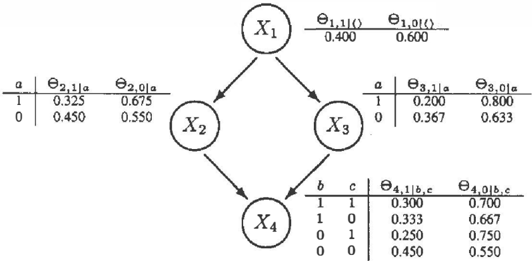
Figure 1 provides a simple example of a belief network with specific CPtable entries. Here X1 has no parents, so we write F 1 = (}.We have F2 :::��: {Xt), Fa= (Xt), F4 = {X2, X a); and for each value a, b, c, d, we have 01, a l 0 = Pr{ xl = a IE>}, e2,bJa = Pr{ x2 = b I Xt = a, E> }, and e4,djb,c = P r { x4 = d I x2 = b, X a = c, e }.
(Hence, using Figure 1, we have 81,1 1 0 = 0.4.) Note that the values in each row add up to 1. In general, the variables need not be binary, but can have larger (finite) domains.
The CPtable entries are estimated using training data and (possibly) expert opinion. The latter information is incor porated using the Bayesian paradigm, where 8 is mod eled as a random variable and expert opinion is expressed through an a priori distribution for 8. We adopt indepen dent Dirichlet priors 1 for the various CPtable rows. Specit1cally, let 8vl/ = (9v,zl/ ) x EX. denote the CPtable row for F v = fe.g., e4J(1,0) = (04,1](1,0), 04,0](1,0}) denotes the entries for the X4 variable associated with the parental assignment X2 = 1 and X3 = 0. We assume that, be fore observing the training data, the evil are independent "Dir( a::,,11, x E Xv )"random vectors, where a:;,,11 > 0. An absence of expert opinion is often expressed by setting a;, x lf = 1 for all (v,x, f)e.g., 84J(1,o) ""Dir( I, 1) -which yields a uniform (flat) prior. Stronger opinion is expressed through larger values of a:* 11. Expressions for v ,x the mean and variance of a Dirichlet distribution are given below.
Now suppose that the training data consist of m indepen dent replicates of vectors X, generated using the given structure and a fixed set of CPtable entries e. Let mv,xlf denote the number of cases in the training set with (Xv, Fv) = (x, f). Under the posterior distribution (the conditional distribution given the training data), the E>vlf are independent Vir( O:v,zl/· x E Xv) random vectors, with O:v,xl f = a;, x l f + mv,xlf [BFH95]. This posterior distri bution underlies our derivation of Bayesian credible inter vals. Several properties of the Dirichlet distribution will be needed.
Setting O:v,. J / = l:: x E Xv O:v, x J f · the posterior means and (co)variances for CPtable entries are [BFH95]:
1 Readers unfamiliar with these assumptions, or with Dirichlet distributions, are referred to [Hec98]. Note that a Dirichlet distri bution over a binary variable is a Beta distribution.
where c5xy = 1 if x == y and c5,y = 0 otherwise. The ran dom vectors Elvlf are asymptotically normal, in the limit as min, av,x l ! --t oo [Aki96]. More precisely, the nor malized variables ..;av, .1f(8v , x1J -1-Lv , x JJ ) converge in distribution to jointly normal random variables with mean zero and covariances J.tv,xJJ(o,y- J.tv ,y JJ ). This asymp totic framework is applicable as the amount of training data increases (m --t oo) provided all of the CPtable entries 8v,xJJ are positive. This condition occurs with probability one under a Dirichlet prior.
3 Bayesian Credible Intervals for Query Re sponses
It is well-known that the CPtable entries determine the joint distribution of X: Pr{ Xv = Xv, v E vIe} = I1vEV ev,x. II.] where(! vlvEV is determined by (x v ) vE V ; see [Pea88]. Users are typically interested in one or more specific "queries" asked of this joint distribution, where a query is expressed as a conditional probability of the form
where H and E are subvectors of X, and h and e are legal assignments to these subvectors. Note also the dependency one.
In our Bayesian context, Q is a random variable with a (the oretically) known distribution determined by the posterior distribution of e. For a point estimate of Q, one may use the posterior mean J.LQ = E { Q}. This value can be calcu lated using the i d e n tity [CH92]:
Set It = E{E>} where the components J.tv,zJ/ of 11are defined by Equation 1.
While a point estimate 11-Q = q(�t) can be useful, one often requires some information concerning the potential error in the estimate. In the Bayesian context, this can be achieved by plotting the posterior distribution of Q. Alternatively, one may construct a 100(1 -r5 ) % credi ble interval for Q; i.e., an interval (L, U) defined so that Pr{ L :::; Q :::; U} = 1 -o. Exact calculations are typi cally not analytically tractable, but simple approximations are available. We w ill show that the distribution of Q is approximately normal, and derive an approximation i7Q for the standard deviation of Q. We then propose the following interval as an approximate 100(1 -r5)% credible interval:
where zo/2 = <I>- 1 (1 -8/2) is the upper J /2 value of the standard normal distribution.
Our derivation is based on a first-order Taylor expansion of q(E>) about q(�J-). Some notation is needed to express the partial derivatives. Let Pv ( h, x, f I e) denote the probabil ity
and let p v ( x , f le),Pv(h,f le),pv(f le), andp(h le) be defined in a similar manner. Note that the subscript v is needed to identify the node when Xv or F u is involved, and all probabilities are evaluated at e = /-£. Let q� . zl / denote the partial derivative 8q(B)/8Bv , z l f evaluated at 0 := IL· We will use the following identity, derived by [GGS97, DarOO]:
We now derive an expression for i7�, and demonstrate asymptotic validity of the credible interval (Equation 4) given a sufficiently large training sample.
Theorem 1 We assume that 8 is a random vector with posterior Dirichlet distribution described in Section 2, and approximate the variance of Q = q(8) by
where
Consider an asymptotic framework where the poste rior means J.t v,xlf are fixed, positive values, and min { nv, z l /} -+ oo. T hen the random variable (QJ.L Q)/i7Q converges in distribution to the standard nonnal distribution.
Proof. Our proof uses the Delta method [BFH95]. Con sider the Taylor expansion
where
and the remainder term R can be expressed in terms of the matrix of second derivatives of q( e) evaluated at a pointe between Band J.t. Since the variances for E>u,zJ! in EqUCJ tion 2 are of order 1/av,zlf --t 0, and since the second derivatives remain bounded in a neighbourhood of f.i, the remainder R is asymptotically negligible compared with D.
We define &b to be the variance of D (Equation 7). As the CPtable rows El vlf are statistically independent, but
二
一
entries within a row are correlated, the variance of D can be expressed as
After substituting Equation 2 for the covariances and sim plifying, we obtain Equation 6 with
A substitution of Equation 5 then yields the equivalent ex pressions/or Avt and Bvt within Equation 6.
We observe that Dfuq is a random variable with mean 0 and variance 1. It remains to show that D / ij Q is asymp totically normal. This result follows from the asymptotic multivariate normality of the components of 8 (after suit able standardization- see Section 2), and the fact that D is a linear function ofEl. 0
Degenerate Case: There are exceptional situations where the posterior distribution of q(9) is analytically tractable and exact credible intervals are available. In the degener ate situation where the network structure has arcs connect ing all pairs of nodes (and hence imposes no assumptions about conditional independence), the assumption of inde pendent Dirichlet distributions for CPtable rows is equiva lent to an assumption of a single Dirichlet distribution over unconditional probabilities Pr{ Xv = Xv, v E V}. It is then straightforward to derive the distribution of the query probability using properties of the Dirichlet distribution; see [Mus93].2 Note that this exact approach is not cor rect in general -i.e., it does not hold for networks with non-trivial structure.3
Computational Issues: The computational problem of computing J.LQ = q(p,) is known to be NP-hard [Coo90]; when all variables Xv are binary, the most effective ex act algorithms require time O(n2w), where n = l VI is the number of nodes and w is the induced tree width of the graph [Dec98, LS99]. The variance uq can also be com puted in time O(n2w). This result follows from the exis tence of algorithms that can compute all of the derivatives
2 Assuming a uniform prior and a sample of size m, we can compute the posterior variance of Pr{ HIE} as P{HIE} x (1F{HIE} )/((m x P{E})+3), where F(x) is the expected value of x, wrt the given belief net.
3 This follows from a dimensionality argument: in a non-trivial structure, the 2n-dimensional vector of unconditional probabili ties is constrained to lie in a lower-dimensional submanifold of t � e 2n -!-dimensional simplex. This cannot be represented by a smgle Dirichlet distribution because, wpl, the constraints would not be satisfied.
| d | Mean | Std.Dev. |
|---|---|---|
| 10% | 2.38 | 1.86 |
| 20% | 3.15 | 2.41 |
| 30% | 3.63 | 2.79 |
| 40% | 3.88 | 2.96 |
q� , xlf in time O(n2w); see [DarOO]. Given these deriva tives, the summations in Equation 6 can be performed with one additional pass over the values, of time 0 ( n).
The extended paper [VGHOl] describes an algorithm for computing UQ. The main challenge, computing all of the derivatives q� x l f' is accomplished by "back propagat ing" intermediate' results obtained by the Bucket Elimina tion [Dec 9 8] algorithm.
[VGHOl] also provides additional comments on the proper interpretation and application of this theorem.
4 Empirical Study
Theorem 1 proves that the interval /-LQ ± z6; 2 uq is asymp totically valid. More precisely, let
be the probability that the query response Q falls outside of the credible interval, based on our UQ estimate of standard deviation, Equation 6. The values 1 -o and 1 -� are the nominal and actual coverage probabilities for the credible interval. The value� is a function of o, the graph (V, A), the query q, and the posterior distribution of 0. The pos terior distribution depends on the prior distribution and the training sample. Thus � typically varies from one applica tion to the next. While Theorem 1 implies that � � o when the training sample is sufficiently large, it does not tell us whether this approximation is valid in practice, particularly for small samples. In general, the validity of the approxi mation depends on all of the factors determining �. We carried out a number of experiments to assess how these factors affect validity.
Given a fixed set of factors, we estimate the correspond ing� by a simple Monte Carlo strategy. Using the ( fixed) posterior distribution of 0, calculate ILQ and uq. Simulate r replicates ei from the posterior distribution, calculate Qi = q(0;), then let.&. be the proportion of the { Qi} with IQ; -/-LQ I > Zof2UQ. In our experiments, each � was based on r = 100 replicates.
To quantify the validity of the approximation� � o, we employ average absolute differences:
The absolute differences are averaged as we vary one or more of the the factors determining �The validity es timates are presented as percentages in our tables. When
1
Standard Normal Ouanmea
(B) QQ-plot showing relation to Normal
viewing these values, it is helpful to have a gold standard for comparison. Consider the validity estimate 1.& - 51 fo r a single ..:l. The minimum expected value is obtained when ..:l == S; i.e., when 100.& has the Binomial(lOO, S) distribu tion. Table 1 presents means and standard deviations under these ideal circumstances. Now suppose a validity estimate is obtained by averaging k ind e p e n de nt terms. Its standard deviation is typically greater than the value Std.Dev./ v'k suggested by Table 1 because there is usually variation in the underlying � values.
4.1 Results for the Diamond Graph
We studied the following inferential patterns in the dia mond graph (Figure I):
The six queries cover a range of different inferential pat terns. The first is basically a "sanity check", as it is a triv ial inference; the fourth is also straightforward, although it does involve a multiplication. The sixth is slightly more complex, but it is still only a summation of a set of prod ucts. The remaining queries involve divisions of increas ingly complicated expressions.
For each m E {10, 20, 30, 4 0 } , we carried out 30 trials of the form: (1) generate E> from a uniform Dirichlet prior distribution, (2) generate a training sample of size m based on E> and use the result to obtain a posterior dis tribution, (3) generate 100 Monte Carlo replicates from the posterior distribution and use these to obtain an esti mate 6. for each pair (Q, J), for Q E {QI. ... , Q6} and
J E {10%, 20%, 30%, 40% }. The resulting validity es timates are listed in Table 2. Each cell in the table is an average of 30 values .
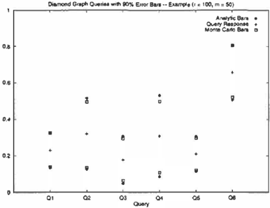
Figure 2(A) shows the error-bars returned by our approx imation, and also the Monte Carlo system, on a random network posterior, for the error-bars for 90% credible inter vals. We see the two methods give similar answers.
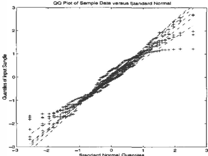
Figure 2(B) uses a quantile-quantile (QQ) plot to address the validity of the normality assumption, independently of the linear approximation. Each "line" in this figure corre sponds to z-scores of the 100 query responses generated by our Monte Carlo simulation, plotted against standard normal quantiles. This figure shows six such lines, each corresponding to a single query in { Q1, . .. , Q6}, given a sample of size m = 10. A straight-line would correspond to data produced by a "perfect" normal distribution; we see each dataset is close. (Of course, this is only suggestive; the real proof comes first from Theorem 1, and then from the data (e.g., Table 2) which demonstrates that our approach, which assumes normality, produces reasonable results.)
4.2 Results for Alarm Network
The Alarm network [BSCC89] is a benchmark network based on a medical diagnosis domain, commonly used in belief network studies. The network variables are all dis crete, but many range over 3 or more values. The network includes a CPtable for each node; i.e., a particular 0 is spec ified.
Table 3 summarizes the results for experiments on the Alarm network, where we varied both J and m. For each m, we generated a single random sample of size m from 0, and used this to determine a posterior distribution (as suming a uniform prior). Validity estimates were obtained by averaging over randomly chosen queries. The queries Pr{H =hIE= e, 0} were chosen by determining an as signment H = h to one randomly chosen query variable, and assignments E = e to five randomly chosen evidence variables. (Here, we used [HC91] to determine which vari-
| m Ql | Q2 | Q3 | Q4 | Q5 | Q6 |
| 6 = 10% | |||||
|---|---|---|---|---|---|
| 10 2.37 | 2.77 | 3.10 | 3.27 | 2.20 | 3.93 |
| 20 2.67 | 3.33 | 2.50 | 3.37 | 2.60 | 3 .50 |
| 30 2.60 | 3.03 | 2.40 | 3.13 | 2.90 | 3.70 |
| 40 2.60 | 2.97 | 3.10 | 2.00 | 2.77 | 2.90 |
| 6 = 20% | |||||
| 10 3.50 | 5.00 | 4.70 | 4.87 | 3.43 | 5.57 |
| 20 4.60 | 6.27 | 5.13 | 7.03 | 4.03 | 4.53 |
| 30 2.90 | 5.07 | 4.43 | 5.97 | 3.97 | 4.87 |
| 40 4.07 | 5.27 | 4.93 | 4.93 | 4;03 | 3.87 |
| 6 = 30% | |||||
| 10 3.63 | 5.63 | 6.10 | 7.23 | 5.13 | 6.27 |
| 20 4.70 | 7.20 | 6.83 | 11.13 | 5.30 | 6.03 |
| 30 3 . 7 0 | 5.80 | 5.47 | 7.20 | 3.50 | 5.30 |
| 40 5.13 | 6.97 | 6.03 | 6.63 | 4.27 | 4.27 |
| 6 = 40% | |||||
| 10 4.33 | 3.97 | 5.33 | 7.53 | 4.40 | 6.63 |
| 20 4 . 73 | 5.20 | 5.73 | 9.27 | 5.20 | 5.97 |
| 30 3.33 | 4.50 | 5.00 | 6.47 | 4.27 | 4.97 |
| 40 3.90 | 4.90 | 5.97 | 6.73 | 4.43 | 4.47 |
| m | 10% | 20% | 30% | 40% |
|---|---|---|---|---|
| 50 | 2.47 | 4.37 | 4.48 | 4.07 |
| 100 | 2.66 | 4.95 | 5.97 | 4.87 |
| 150 | 3.04 | 5.35 | 6.45 | 5.66 |
| 200 | 2.65 | 4.80 | 5.43 | 5.42 |
abies could be query as opposed to evidence variables.) Some or all of the evidence variables might have had no effect on the query variable, others might have had a pro found effect. Each cell in Table 3 represents an average from 100 queries on a single posterior distribution.
4.3 Results for Random Networks
Although random networks tend not to reflect typical (or natural) domains, they complement more focussed studies by exposing methods to a wide range of inputs and help to support claims of generality. We carried out experiments on networks with 10 binary variables and 20 links, gener ating gold models from a uniform prior distribution on e. and generating random queries of various types. Here we used sample size m = 100 throughout, and varied the type of query. Table 4 displays the results of our experiments. Each query was of the form Pr{H =hIE= e, 9}, with varying dimensionalities forE and H. Let #E and #H denote the number of variables comprising E and H, re spectively. Each cell of Table 4 is based on 100 trials: I 0 queries on 10 networks, with both structure and posterior generated randomly.
| #E | ||||
|---|---|---|---|---|
| #H | 2 | 3 | 4 | 5 |
| 10% | ||||
| = | 0 | 3.20 | ||
| 1 2.16 2.59 | 2.72 | 2.84 | 3.00 | |
| 2 | 2.50 | 2.9 3 | 3.13 | 2.45 |
| 3 2.49 | 2.59 | 2.62 | 2.38 | 2.56 |
| 4 2.57 | 2.26 | 2.S4 | 2.58 | 2.88 |
| 5 2.72 | 2.53 | 2.61 | 3.05 | 2.79 |
| 6 = 20% | ||||
| 1 3.06 | 4.16 | 4.41 | 4.19 | 4.39 |
| 2 3.60 | 3.63 | 4.38 | 4.71 | 4.96 |
| 3 3.50 | 4.16 | 4.56 | 5.07 | 5.78 |
| 4 4.12 | 4.46 | 5.64 | 6.31 | 7.14 |
| 5 4.67 | 5.76 | 6.63 | 7.85 | 8.17 |
| 0 = 30% | ||||
| 1 4.17 | 4. 7 8 | 5.11 | 4.75 | 5.97 |
| 2 4.46 | 4. 2 8 | 5.02 | 5.13 | 6.33 |
| 3 4.12 | 4.74 | 5.14 | 6.39 | 7.25 |
| 4 4.98 | 5.61 | 7.43 | 8.71 | 10.81 |
| 5 5.69 | 7.63 | 9.45 | 12.51 | 13.99 |
| 0 = 40% | ||||
| 1 4.20 | 4.90 | 5.00 | 4.56 | 5.62 |
| 2 4.43 | 4.24 | 4.81 | 5.44 | 6.43 |
| 3 4.11 | 4.62 | 4.80 | 5.95 | 7.12 |
| 4 5.15 | 4.52 | 6.47 | 8.36 | 10.99 |
| 5 4.95 | 7.14 | 8.95 | 13.05 | 16.15 |
4.4 Discussion
Our hypothesis was that our Bayesian error-bars algorithm would be accurate for essentially all cases. We tried to falsify our hypothesis by varying the following experimental factors:
- Network structure (V, A)
- Credibility level 1 -c5
- Query type (Diamond network, Alarm)
- Number of evidence variables (Random networks)
- Number of query variables (Random networks)
In no case did we observe a result where averagelto -81 exceeded 20%. In most cases, the validity estimate was less than 8/3. As noted in Table 1, even if our error-bars were exact, we would still get positive validity estimates due to the variance in to about �-We therefore believe that these results comfortably bound the expected error of our method under the experimental conditions. None of the factors that we manipulated had a profound effect. T he strongest ef fect, observed in Table 4, was that increasing the number of variables assigned in a query tended to increase the er ror I� -81; see also [Kle96]. One possible explanation is that, as #E and #H increase, the query function q tends to become more complex, and the local linear approxima tion of q becomes less reliable. Another possibility is that
the query probability Q tends to become very small, mak ing the normal approximation less accurate. Further exper iments could address this issue.
We found these results very encouraging. Our method appears to give reasonable error-bars for a wide range of queries and network types. This makes the technique a promising addition to the array of data-analysis tools re lated to belief networks, especially as the algorithm is rea sonably efficient, (only) roughly doubling the computation time per inference. While there may be pathological cases where our method will not give reasonable results - per haps because the local linear approximation and the asymp totic normality are far off the truth we did not find such cases in our experiments.
Other Experiments: We also ran a number of other ex periments. One set computed the average { A -8} scores in each situation, to determine if there was any systematic bias. (Note this score differs from Equation 9 by not tak ing absolute values.) We found that our bounds were typi cally a bit too wide for most queriesi.e., we often found the 1 -a-interval included slightly more than 1 -8 of the cases. We are currently investigating this, to see if there are straight-forward refinements we can incorporate.
We also computed error-bars based on the (incorrect!) "complete structure" assumption, which implies the re sponse will have a simple Dirichlet distribution; see Foot note 2. We found that, as anticipated, the approach de scribed in this paper, using Equation 6, consistently out performed that case, in that our approach was consistently closer to the Monte Carlo estimates.
[VGHOl] discusses these results in detail. It also inves tigates techniques for dealing with extreme values, where the normal distribution may be sub-optimal.
5 Related Work
Our results provide a way to compute the variance of a BN's response to a query, which depends on the posterior distribution over the space of CPtable entries, based on a data sample. This is done using the "Delta method" [BFH95]: first determine the variance of each CPtable row, then propagate this variance using a sensi tivity analysis (i.e., the partial derivatives); see Equation 6. Kleiter [Kle96] performs a similar computation; parts of his analysis are more general, in that he considers incomplete data. However, he does not (1) discuss how to deal with general graphical structures, (2) show how to deal with the correlations encountered with general Dirichlet distri butions, nor (3) provide an efficient way to compute this information. Moreover, our empirical data provide addi tional evidence that the approximations inherent in this ap proach are appropriate, even for small sample sizes.
Several other researchers also consider the posterior distri- bution over CPtables, but for different purposes. For exam ple, Cooper and Herskovits [CH92] use it to compute the expected response to a query; by contrast, we also approx imate the posterior variance in that response. Similarly, while many BN-learning algorithms compute the posterior distribution over CPtables [Hec98], most of these systems seek a single set of CPtable entries that maximize the like lihood, which again is different from our task; e.g., their task is not relative to a specific query (but see [GGS97]).
Many other projects consider sensitivity analyses, provid ing mechanisms for propagating ranges of CPtable values to produce a range in the response; cf., [BKRK97, Las95, CNKE93, DarOO]. While these papers assume the user is explicitly specifying the range of a local CPtable value, our work considers the source of these variances based on a data sample. This also means our system must propagate all of the "ranges"; most other analyses consider only prop agating a single range. The [DarOO] system is an excep tion, as it can simultaneously produce all of the derivatives. However, Darwiche does not consider our error-bar appli cation, and so does not include the additional optimizations we could incorporate.
Excluding the [DarOO] result, none of the other projects provides an efficient way to compute that information. Also, some of those other papers focus on properties of this derivative - e.g., when it is 0 for some specific CPt able entry. Note that this information falls out immedi ately from our expression (Equation 6). Finally, our anal ysis holds for arbitrary structures; by constrast some other results (e.g., [CNKE93]) deal only with singly connected networks (trees).
Lastly, our analysis also connects to work on abstractions, which also involves determining how influential a CPtable entry is, with respect to a query, towards deciding whether to include a specific node or arc [GDSOl]. Their goal is typically computational efficiency in computing that re sponse. By contrast, our focus is in computing the error bars around the response, independent of the time required to determine that result.
6 Conclusion
Further Extensions: Our current system has been im plemented, and works very effectively. There are several obvious ways to extend it. One set of extensions corre spond to discharging assumptions underlying Theorem 1: computing error bars when the data was used to learn the structure, as well as the parameters; dealing with param eters that are drawn from a distribution other than inde pendent Dirichlets, perhaps even variables that have con tinuous domains; dealing with a training sample whose instances are not completely specified. Our work deals with fully-parameterized CP tables. It would be interesting to investigate techniques capable of dealing with CPtables
一
represented as, say, decision tree functions [BFGK96], etc.
Contributions: Many real-world systems work by rea soning probabilistically, based on a given belief net modeL When knowledge concerning model parameters is condi tioned on a random training sample, it is useful to view the parameters as random variables; this characterizes our uncertainty concerning the responses generated to specific queries in terms of random variation. Bayesian error-bars provide a useful summary of our current knowledge about questions of interest, and so provide valuable guidance for decision-making or learning.
This paper addresses the challenge of computing the error bars around a belief net's response to a query, from a Bayesian perspective. We first motivated and formally de fined this task- finding the 100(1 - o)% credible interval for a query response with respect to its posterior distribu tion, conditioned on a training sample. We then investi gated an application of the "Delta method" to derive these intervals. This required determining both the covariance matrix interrelating all of the parameters, and the derivative of the query response with respect to each parameter. We produced an effective system that computes these quanti ties, and then combines them to produce the error-bars.
The fact that our approximation is guaranteed to be cor rect in the limit does not mean it will work well in practice. We therefore empirically investigated these claims, by test ing our system across a variety of different belief nets and queries, and over a range of sample sizes and credibility levels. We found that the method works well throughout.
Acknowledgements
We are grateful for the many comments and suggestions we received from Adnan Darwiche and the anonymous review ers, and for the fairness of the UAI'01 programme chairs. All authors greatfutly acknowledge the generous support provided by NSERC, iCORE and Siemens Corporate Re search. Most of this work was done while the first author was a student at the University of Alberta.
References
- [Aki96] Y. Akimoto. A note on uniform asymptotic nor mality of Dirichlet distribution. Mathematica Japonica, 44:25-30, 1996.
- [BFGK96] C. Boutilier, N. Friedman, M. Goldszmidt, and D. Koller. Context-specific independence in Bayesian networks. In UAI-96, 1996.
- [BFH95] Y. Bishop, S. Fienberg, and P. Holland. Dis crete Multivariate AnalysisTheory and Practice. MIT Press, 1995.
- [BKRK97] J. Binder, D. Koller, S. Russell, and Ke. Kanazawa. Adaptive probabilistic networks with hidden variables. Machine Learning, 29:213-244, 1997.
- [BSCC89] I. Beinlich, H. Suermondt, R. Chavez, and G. Cooper. The ALARM monitoring system: A case study with two probabilistic inference techniques for be lief networks. In Proc. Second European Conf Artificial Intelligence in Medicine, August 1989.
- [CH92] G. Cooper and E. Herskovits. A Bayesian method for the induction of probabilistic networks from data. MU, 9:309-347, 1992.
- [CNKE93] P. Che, R. Neapolitan, J. Kenevan, and M. Evens. An implementation of a method for com puting the uncertainty in inferred probabilities in belief networks. In UA/-93, pages 292-300, 1993.
- [Coo90] G. Cooper. The computational complexity of probabilistic inference using Bayesian belief networks. Artificial Intelligence, 42(2-3):393--405, 1990.
- [DarOO] A Darwiche. A differential approach to inference in bayesian networks. In UA/'00, 2000.
- [Dec98] R. Dechter. Bucket elimination: A unifying framework for probabilistic inference. In Learning and Inference in Graphical Models, 1998.
- [GDSOl] R. Greiner, C. Darken, and I. Santoso. Efficient reasoning. Computing Surveys, 33:1-30,2001.
- [GGS97] R. Greiner, A Grove, and D. Schuurmans. Learning Bayesian nets that perform welL In UAI-97, 1997.
- [HC91] E. Herskovits and C. Cooper. Algorithms for Bayesian belief-network precomputation. In Methods of Information in Medicine, pages 362-370, 1991.
- [Hec95] March 1995. Special issue of "Communications of the ACM", on Bayesian Networks.
- [Hec98] D. Heckerman. A tutorial on learning with Bayesian networks. In Learning in Graphical Models, 1998.
- [Kle96] G. Kleiter. P ropagating imprecise probabilities in bayesian networks. Artificial Intelligence, 88, 1996.
- [Las95] K. Laskey. Sensitivity analysis for probability as sessments in Bayesian networks. IEEE Transactions on Man, Cybernetics and Systems, 25(6):901-909, 1995.
- [LS99] V. Lepar and P. P. Shenoy. A comparison of Lauritzen-Spiegelhalter, Hugin, and Shenoy-Shafer ar chitectures for computing marginals of probability dis tributions. In UA/98, 1999.
- [Mus93] R. Musick. Minimal assumption distribution propagation in belief networks. In UA/93, 1993.
- [Pea88] J. Pearl. Probabilistic Reasoning in Intelligent Systems: Networks of Plausible Inference. Morgan Kaufmann, 1988.
- [VGH01] T. Van Allen, R. Greiner, and P. Hooper. Bayesian error-bars for belief net inference. Technical report, University of Alberta, 2001.