Bayesian Networks for Dependability Analysis: an Application to Digital Control Reliability

Luigi Portinale and Andrea Bobbio

Dipartimento di Scienze e Tecnologie A vanzate

Universita del Piemonte Orientale " A. Avogadro" - Alessandria (ITALY)

Abstract

Bayesian Networks (BN) provide robust probabilistic methods of reasoning under un­ certainty, but despite their formal grounds are strictly based on the notion of condi­ tional dependence, not much attention has been paid so far to their use in dependability analysis. The aim of this paper is to pro­ pose BN as a suitable tool for dependability analysis, by challenging the formalism with basic issues arising in dependability tasks. We will discuss how both modeling and anal­ ysis issues can be naturally dealt with by BN. Moreover, we will show how some limi­ tations intrinsic to combinatorial dependabil­ ity methods such as Fault Trees can be over­ come using BN. This will be pursued through the study of a real-world example concerning the reliability analysis of a redundant digital Programmable Logic Controller (PLC) with majority voting 2:3

1 Introduction

Dependability analysis involves a set of methodologies dealing with the reliability aspects of large, safety­ critical systems [9, 10]. Two main categories of ap­ proaches can be identified: combinatorial methods and state-space based methods. The first category requires a description of the system to be analyzed in terms of components and their interactions. In particular, com­ ponents are modeled as binary events corresponding to component up and component down respectively, while interactions are usually described by means of boolean AND/OR gates. The advantage of such techniques is that they are component-oriented and that simple for­ malisms like Fault Trees (FT) can be adopted. How­ ever, some major simplificative assumptions are usu­ ally needed, both at the modeling and analysis level.

On the contrary, state-space approaches rely on the specification of the whole set of possible states of the system and on the modeling of the possible transi­ tions among them. Markov Chain methods are usu­ ally adopted in this case, giving the analyst the pos­ sibility of explicitly considering all possible interac­ tions among components. The main disadvantage is that, even for not very large systems, using directly the approach may be unfeasable due to the huge di­ mensionality of the considered state-space. The usual solutions is then to resort to partial state descriptions like Petri Nets [11] or Bayesian Networks based mod­ els [5] . However, state-space approaches are essen­ tially used when emphasis is on temporal evolution of the systems, while combinatorial methods concen­ trate more on static aspects as the logical interactions of the components1.

In this paper we aim at considering combinatorial methods for dependability analysis, by showing how basic problems addressed by the approach can be prof­ itably dealt with by using Bayesian Networks. In particular we will concentrate on Fault Tree Analysis (FTA) and on the modeling and analysis issues that are involved in this task. We will show that any FT can be mapped into a BN and that any analysis that can be performed on the FT can be performed by means of BN inference. In addition, standard modeling tech­ nique of BN like noisy gates, multi-state variables or common cause identification, can overcome some basic modeling limitations of fault-trees , while interesting analysis neglected in FTA can be naturally obtained by classical BN inference.

The paper is organized as follows: section 2 discusses basics of fault-tree analysis, while in section 3 an al­ gorithm for mapping a FT into a BN is proposed; in section 4 the suitability of a BN for dependability anal­ ysis is investigated and in section 5 basic extensions to

1

As we will see, this does not means that time is not considered, but only that temporal evolution is not directly modeled.

FTA provided by Bayesian networks are discussed, to­ gether with the improvements they provide both at the modeling and at the analysis level.

2 Fault-Tree Analysis

Combinatorial models of dependability have a poor modeling power coupled with a high analytical tractability based on the assumption of statistically in­ dependent component. Among them, Fault-Tree Anal­ ysis {FTA) has become very popular for the analysis of large safety-critical systems [9, 10]. The goal of FTA is to represent the combination of elementary causes, called the primary events, that lead to the occurrence of an undesired catastrophic event, the so called Top Event (TE). FTA is carried out in two steps: a quali­ tative step, in which the list of all the possible combi­ nations of primary events (the minimal cut-sets) that give rise to the TE is determined and a quantitative step where, if probability values can be assigned ( di­ rectly or by computation) to all the events appearing in the tree, the probability of occurrence of the TE can also be calculated.

The qualitative analysis step is considered very im­ portant in dependability analysis and safety studies, since it allows the analyst to enumerate all the possi­ ble causes of failure for the system and to rank them according to a very simple severity measure given by the (prior) failure probabilities of components. How­ ever, because of the simplicity of the model, only prior failure probability can be considered and no kind of scenarios more specific than cut-sets can be computed.

The major weak point of the FTA methodology (as well as of any combinatorial technique), is the fact that the events must be considered as statistically indepen­ dent. The aim of the present paper is to show that, even by representing knowledge as in combinatorial models, alternative formalisms like Bayesian networks can be profitably adopted to overcome their limita­ tions. Let us now introduce some basic notions con­ cerning FTA:

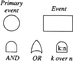
Definition 1 A fault tree {FT) is a tree comprising five types of nodes: primary events, events, two types of elementary logical gates, namely AND gates and OR gates, and one derived logical gate, namely the k out of n gate k: n {see Figure 1).

The root of a FT is an event called the Top Event (TE), representing the failure of the whole system. Each event has exactly one successor which can be ei­ ther a primary event or a logical gate. A logical gate has two or more successors, which are all events; a k out of n gate has exactly n successor events. The leaves of the tree are all primary events.

k over n

Figure 2: The PLC Case Study

The events considered in any FT are binary events, that is they may just assume logical values true or false. Since events are used to represent the func­ tional behavior of a given sub-system, the logical val­ ues are put in correspondence with faulty and working behavior respectively. In particular, primary events are associated to system components. A FT is then constructed by combining primary and general events with logical gates, in order to model the functional behavior of the whole system to be analyzed.

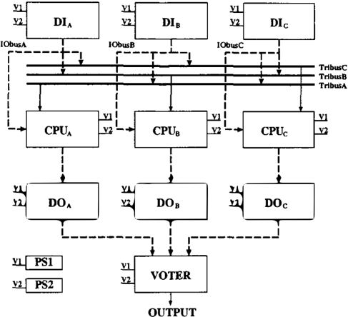
Examp l e 1. Let use introduce a simple but real PLC system, that we will use as a case study throughout the paper. The block diagram of such a system is shown in figure 2. The PLC system is intended to process a digi­ tal signal by means of suitable processing units; in par­ ticular, a redundancy technique is adopted, in order to achieve fault tolerance, so three different channels are used to process the signal and a voter hardware device, with majority voting 2 : 3, is collecting channel results to produce the output. For each channel (identified

三

as channels ChA, Chn and Chc respectively) a digital input unit (DI), a processing unit (CPU) and a digi­ tal output unit (DO) are employed. The digital signal elaborated by a given channel is transmitted among units through a special bus called lObus. Moreover, redundancy is present also at the CPU level; indeed, each CPU receives from its digital input unit the sig­ nal to be elaborated, but it also receives a copy of the signal from other input channels. For doing this, a bunch of three buses is used, called TribusA, Tribusn and Tribusc respectively; the !Obusx of channel Chx delivers the signal of the digital input of channel Chx (Dlx) to tri-buses of other channels (i.e. to Tribusy with Y # X) and CPU x reads the signal from other input channels from Tribusx. Each CPU performs then a software majority voting 2 : 3 for determining the input signal. Finally, the system is completed by a redundancy on the power supply system: two indepen­ dent power supply units ( P S1 and P S 2 ) are connected to other components, in such a way that the simulta­ neous failure of both P S units is needed to prevent the system to work.

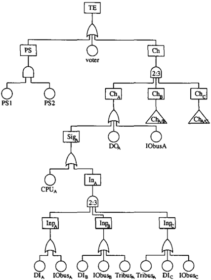
The FT for this PLC system is reported in figure 3. Notice that 2 : 3 gates are used to model the fault of the input part of each channel (since each CPU adopts a 2 : 3 majority voting) and the fault corre­ sponding to the fault of at least 2 channels (since the voter also uses a 2 : 3 majority voting). Notice also that sub-trees rooted at a given channel X are sim­ ilarly replicated for other channel different from X; indeed, notation ChA/B and ChA/C is used to indi­ cate that sub-trees rooted at Chn and Chc are equal to the sub-tree rooted at ChA with A substituted with B and C respecti vely 2 ·

Given a model like the FT of figure 3, some typical analysis can be performed.

Qualitative Analysis. Given the FT, to determine the minimal cut-sets (MCS), i.e. the minimal (with respect to set inc! usion) set of primary events causing the occurrence of the TE(the prime implicants of the TE).

Quantitative Analysis. i) Given probabilistic in­ formation about truth of primary events (i.e. about failure of components), to determine the probability of occurrence of any event in the FT and in particular of the TE. ii) Given MCS, to determine their impor­ tance, also called their unreliability.

MCS determination is usually based on minimization techniques on the set of boolean functions represented by the gates of the FT. The cardinality of a cut-set is called its order. The FT of figure 3 has 59 MCS, one of order I (corresponding to the voter faulty) and the remaining 58 of order 2. For instance, a MCS of order 2 that can immediately be derived from the FT of fig­ ure 3 is {PS1, PS2} corresponding to the simultaneous failure of both power suppliers.

Concerning quantitative analysis, the most common assumption made in FTA is to assume that compo­ nents corresponding to primary events have an expo­ nentially distributed failure time. This means that the probability of having component C faulty at time t (alternatively the probability of occurrence of the primary event C = faulty) is P(C = faulty, t) = I -e->-ct, where >.c is the failure rate of component c.

Given the failure rates of each component, FTA can determine at any time instant t, the probability of oc­ currence of any event and in particular the probability of system failure (the TE) at timet. Moreover, the so­ called unreliability of MCS at timet can be computed. This corresponds to the probability of the joint occur­ rence of events in the cut-set at timet; because of the independence assumption made on the occurrence of primary events, this corresponds to the product of the probability of occurrence of each primary event in the cut-set at time t 3 .

2 Actually events lnpA, lnpB and lnpc have to be dealt appropriately by making a double indexing with respect to the channels; this should be more clear in the following.

30ther kind of quantitative information such as the mean time to failure and the variance of time to failure

Table 1: Failure Rates and Probabilities for PLC Com­ ponents

Component	Failure Rate (f/h)	Failure Prob.
lObus	>.w - 2.0 10 9	0.00080
Tribus	ATri = 2.0 10-9	0.00080
Voter	>-v = 6.6 10-8	0.02605
DO	>-vo = 2.45 Io-7	0.09335
DI	>.DI = 2.8 10-7	0.10595
PS	APS = 3.37 10-7	0.12611
CPU	>.cpu = 4.82 10-7	0.17535

Table 2: Top 11 MCS for PLC System

MCS	Unrel.	Post. Unrel.	Post. P rob.
{CPUA, CPUB}	0.03075	0.13943	0.04533
{CPUB, CPUc}	0.03075	0.13943	0.04533
{CPUA, CPUc}	0.03075	0.13943	0.04533
{Voter}	0.02605	0.11812	0.02681
{CPUA, DOc}	0.01637	0.07423	0.02195
{CPUA, DOB}	0.01637	0.07423	0.02195
{CPUB, DOA}	0.01637	0.07423	0.02195
{CPUB, DOc}	0.01637	0.07423	0.02195
{CPUc, DOA}	0.01637	0.07423	0.02195
{CPUc, DOB}	0.01637	0.07423	0.02195
{PS,, PS2}	0.01590	0.07212	0.02088

Example 2. In the system of figure 2, the fail­ ure rates (in terms of f ailure/hour) shown in ta­ ble 1 can be assumed by considering exponentially distributed failure time. Table 1 also shows the fail­ ure probability of components after 4 · 105 hours of system operation. FTA can then compute the prob­ ability of system failure at time t = 4 · 105 hours as P( TE ) :::: 0.22053. Similarly, the probability of any other event of the FT can be obtained. For example the probability of having a failure in the input part of a channel ( P ( I n x =faulty) = 0.03248, X= A, B, C) or the probability of failure of at least two channels (P(Ch =faulty)= 0.18674 ) .

Finally, MCS can be ranked in order of unreliability; table 2 shows the first 11 MC'S and in the second col­ umn (Unrel.) their corresponding unreliability. We can easily verify that the most critical components are the C' PUs, since the cut-sets involving a failure of at least two CPUs are those showing larger unreliability.

In the next sections we will show that, by using Bayesian networks, besides to perform the above anal­ yses we can augment both the modeling and the anal­ ysis power in dependability tasks.

can be obtained, but this is usually a matter of general reliability analysis not peculiar to FTA.

3 Mapping Fault Trees to Bayesian Networks

Given a FT, it is straightforward to map it into a binary BN, where every variable has two admissible values: false corresponding to a normal or working value and true corresponding to a faulty or not-working value. The conversion can be obtained as follows:

• for each leaf node of the FT, create a root node in the BN; however, if several leaves of the FT represent the same primary event (i.e. the same component), create just one root node in the BN to represent all of them.
• for each pair (gate, output-event) of the FT, create a corresponding node in the BN;
• connects nodes in the BN as corresponding nodes are connected in the FT;
• for each node of the BN created from an AND (re­ spectively OR) gate, create a Conditional Proba­ bility Table (CPT) such that the node is true with probability I iff all parent nodes are true (respec­ tively iff at least one parent node is true);
• for each node created from a k out of n gate, cre­ ate a CPT such that the node is true with prob­ ability 1 iff at least k out of n parent nodes are true.

Prior probabilities on root nodes have to be established by considering a given time point t. Given a root node C, the probability of C = true will be set to the proba­ bility of occurrence of the corresponding primary event at timet (i.e. P(C = faulty), t) = 1e-> -ct). It should be clear that from the above conversion non­ root nodes of the BN are actually deterministic nodes, i.e. special chance (random) nodes with associated a deterministic function for their value determination ( 8 ] .

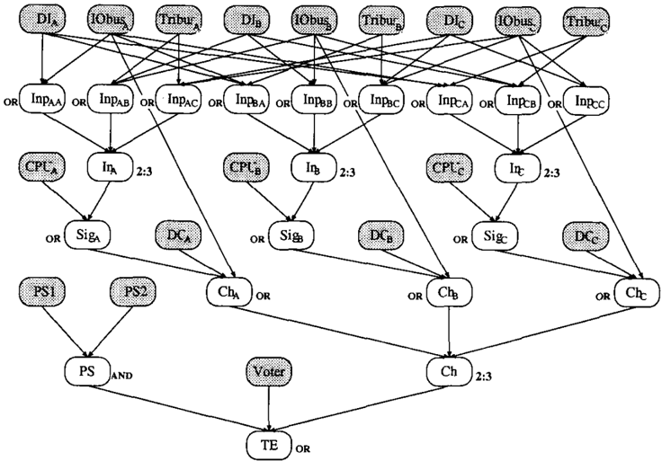
Figure 4 shows the structure of the BN for the PLC system of figure 2 and derived from the FT of figure 3. Random variable nodes (i.e. root nodes) are shown as gray ovals, while deterministic variable nodes are empty ovals. Notice that, as mentioned in section 2, events of type I np actually need two indices to distin­ guish the cases where a Tribus is involved from those where it is not. Prior probabilities for roots can be obtained from table 1 for time t = 4 · 105 hours. Near each deterministic node is indicated the boolean func­ tion represented. The user has just to specify the type of function: CPT specification can then be automati­ cally obtained4.

4 Alternatively, the number of required probabilities can be reduced by techniques like the asymmetric assessment

4 Dependability Analysis with Bayesian Networks

Typical FTA can be performed quite naturally in a BN setting. In particular, concerning MCS determination (i.e. qualitative analysis), because any deterministic node of the BN correspond to a boolean gate of the FT, any kind of technique adopted in FTA for com­ puting MCS can be applied also for the corresponding Bl'f' . However, as we shall see in the following, the BN framework can refine the notion of cut-set when uncertainty about combinatorial knowledge has to be introduced (see section 5). Concerning quantitative analysis, a BN can in principle computes the posterior probability of any set of variables Q given the evidence set E (i.e. P(QIE )), so any kind of probabilistic com­ putation that can be performed in FTA can also be performed by BN inference. In particular the follow­ ing parameters can be computed at timet:

probability of occurrence of an event; it corre­ sponds to the computation of the prior marginal at time t on the node corresponding to the given event;

unreliability of MCS; it corresponds to the compu­ tation of the joint prior on nodes mentioned in the

(6]. 5

More specific techniques relying on the "logical seman­ tics" of a EN in terms of Hom clauses (13, 14] can also be devised, by adopting abductive reasoning.

cut-set at time t6•

Concerning the first point, the marginals of all the fail­ ure events represented in the net can be computed by BN probability propagation [12]. However, standard BN inference usually deals with posterior probability computation, while the above issue are only related to prior information (i.e. to prediction of particular events at timet). In fact, by considering the occur­ rence of a failure, posterior information can be very relevant for dependability and reliability aspects.

Example 3. Suppose the system failure has been ob­ served in the PLC system (i.e. the TE has occurred). A Belief Updating [12] algorithm can be used to com­ pute marginal posteriors on root nodes. Results are summarized in table 3. Notice for instance that, dif­ ferently from the prior information, after observing the fault, a digital output unit is less reliable than a digi­ tal input one; this is reasonable since the difference in prior reliability was very small and the input part of a channel has more redundancy that the output part. This information cannot be directly obtained in FTA; it can be deduced by the fact that cut-sets involving digital output units have a higher unreliability thah those containing digital inputs (see table 2). Marginal posterior probability of nodes corresponding to non primary events (i.e. to sub-systems failure) can simi­ larly be computed.

6 As in FTA this is obtained by multiplying the prior of the true value of each node in the cut-set.

Table 3: Posterior Probabilities for PLC Components

Component	Post. Failure Prob.
Tribus	0.00175
lObus	0.00208
Voter	0.11812
DI	0.17167
PS	0.17603
DO	0.20433
CPU	0.38382

Regarding MCS analysis, BN inference can be more precise than usual FTA; indeed, (Composite) Belief Revzszon [12] algorithms can be used to compute pos­ terior probability of MCS. Even if the ranking provided by prior unreliability of MCS is the same as the one provided by posterior unreliability 7, posterior unrelia­ bility is a more reliable measure. Table 2 reports such � arameters on the third column. Notice that, even 1f such values are in principle computable also with FTA (after the computation of the probability of the TE), FTA tools usually report just the information of table 2.

Finally, composite queries can provide results more specific than MCS; indeed, in a MCS no commitments is made to unmentioned events. More specific informa­ tion can be obtained by setting for query in BN infer­ ence all primary events. If we consider a component­ oriented framework for system analysis (as is done in reliability), then MCS corresponds to partial or kerc nel diagnoses, while a composite query on every pri­ mary event will produce complete diagnoses (in terms of component behavioral modes) [3]. While in a log­ ical setting kernel diagnoses can be suitably adopted for concisely explain a system failure, in probabilistic analysis this is no longer true, since marginalization operations can provide counter-intuitive results [12]. If we interpret each entry of the first column of table 2 as assigning the faulty mode to mentioned components and the working mode to unmentioned ones, we can interpret the MCS as diagnoses whose posterior prob­ ability if given in the last column of the table. Notice that, even if the top 11 diagnoses of our problem ac­ tually correspond to top 11 MCS in the same order of probability, this is not true in general, since diag­ noses corresponding to non-minimal cut-sets may have a larger probability than some diagnoses correspond­ ing to MCS. For instance, even if the PLC system has 59 MCS, the 18th (in order of probability) diagnosis is the one corresponding to all CPUs faulty and every

7Since MCS are prime implicants of the TE the condi­ tional probability of TE given a MCS is 1, so t h e posterior of a MCS given the TE differs from the prior only for the constant P( TE)-1·

other component working (probability 0.00963) and this does not correspond to a MCS.

5 Augmenting Modeling Power

There are essentially three main features of BN for­ malism that may be exploited to improve combina­ torial dependability analysis: noisy gates, multi-state variables and sequential failure dependence.

5.1 Noisy gates

Di � erently from fault-trees, in a BN dependency re­ latwns between events or variables are not restricted to be deterministic. In dependability terms, this cor­ responds to being able to model uncertainty in the behavior of the "gates" that in a FT represent inter­ actions between sub-systems. Of particular attention for reliability aspects is one peculiar modeling feature often used in building BN models: noisy gates. The most common kind of noisy gate is the noisy-or model [12] and its generalizations [7]; this kind of model can be profitably used in dependability, since it allows a simple probabilistic generalization of boolean gates.

Consider, in the PLC case study, a situation in which more fault-tolerance is added to the system by means of a third spare power supplier that is available un­ der certain circumstances; in particular, it is shared by other systems and it is available only if it is not al­ ready in use. In this situation, it is no longer true that when both modeled suppliers are down, also the sys­ tem is certainly down, since the control system could switch to the spare supplier. Suppose that, from sta­ tistical information, we know that the spare supplier is available the 30% of time when the P S sub-system is down: we can model the uncertainty about the avail­ ability of the spare supplier by transforming the gate corresponding to the TE in a noisy-or gate with the following parameters (remember that TE = true means system failure):

As done in [2] we use c instead of P to emphasize the fact that these are not standard conditional proba­ bilities. The noisy-or independence assumption about causes of the TE is in this case reasonable and we could conclude that the system is down when only the PS sub-system is down with probability

corresponding to the percentage of times that the spare supplier is not available, while if all causes are present we obtain

Moreover, another important modeling issue in de­ pendability analysis is the problem usually referred as the common causes problem, where the system may go down, even in the presence of components up. This usually refer to the presence of some common unknown cause of failure that has been neglected in the model. This is naturally treated in a BN by means of leak probabilities [15]. In the above example, we may have that the TE may be true even when both P S, Voter and C h sub-systems are functioning, because of a com­ mon cause problem; by assuming a leak probability l = 1 · 10 -4 the first parameter becomes

and the unreliability of the system when sub-systems PS, Voter and Ch are down becomes

which is slightly larger than in the case where no com­ mon cause problem was present.

Dually from noisy-or, we could also use a noisy-and gate to generalize AND gates of the FT. For instance, by considering the possibility of failure of wire con­ nections from power supply units, we can model the fact that, even if only one supplier is down, the P S sub-system is also down (because connections from the other supplier are not working). More specifically, if we assume that this event has a probability of 0.01, then we can specify the noisy-and as

and then to compute

corresponding to the simultaneous independent failure of connections from both supplier.

5.2 Multi-state variables

The working/faulty dichotomy of FTA can be im­ proved towards the most reasonable approach of deal­ ing with variables having more than two values (multi- state variables). This is particularly useful for primary events, since in this way the system component they refer to can be modeled by means of multiple behav­ ioral modes [4]. In fact, components may manifest more than one failure mode (e.g open/short) and the failure modes may have a very different effect on the system operation (e.g. fail-safe/fail-danger). Suppose to consider a three-state component whose states are identified as working (w), f ail-open (f-o) and fail-short (f-s). In FTA the component failure modes must be modeled as two independent binary events ( w/f-o) and (w/f-s); however, to make the model correct, a (non­ standard) XOR gate must be inserted between f-o and f-s since they are mutually exclusive events. On the contrary, Bayesian networks can include n-ary vari­ ables by adjusting the entries of the CPT. Saving in assessment provided by classical noisy-or in case of bi­ nary variables can now be obtained through general­ izations to n-ary variables, like for instance the noisy­ max gate [15]. In the next subsection we will return more specifically on this point.

5.3 Sequentially Dependent Failures

Another modeling issue that may be quite problem­ atic to deal with by using fault-trees is the problem of components failing in some dependent way. Bayesian networks may address this point by making explicit such a dependency in the structure of the net. Con­ sider for instance the case in which, in the PLC of fig­ ure 2, power suppliers may induce a CPU failure when failing; this can be due to the fact that a possible fault for power supplier is an over-voltage, causing a possible CPU damage (and then a CPU fault). While it is not possible to model this kind of information in a FT, in a BN it can be naturally modeled by connecting each power supplier to the CPU nodes. In particular, one can even be more precise, by resorting to multi-state variable modeling; indeed, each PS; unit (i = 1, 2) can be modeled with three ordered values, working, over.voltage, dead, and connected as a parent to each CPU node C PUx (X = {A, B, C}) with the following noisy-max parameters:

The probability of getting a CPU fault when both the suppliers are in over-voltage can then be computed from noisy-max model as

This shows how a flexible combination of basic features

of a BN can naturally overcome basic limitations of FTA.

Finally, it is worth noting that, if uncertainty about combinatorial knowledge on components has to be modeled ( either through noisy gates simplifications or through complete CPT specifications ) , the FTA notion of MCS does no longer make sense. In this case, the computation of diagnoses intended as composite be­ liefs on primary events as shown in section 4, provides a natural counterpart of the MCS concept.

6 Conclusions

In the present paper we have discussed the suitability of Bayesian networks for classical combinatorial de­ pendability analysis. A preliminary analysis on this topic was proposed in [1] ( where no formal compari­ son with classical dependability analysis was provided ) and in [16] ( where the starting point are reliability block diagrams ) . We have shown that combinato­ rial formalisms like fault-trees can be formally mapped into binary BN and that classical FTA can be natu­ rally performed through BN inference. Basic features of BN allow to overcome limitations of FTA both at the modeling and at the analysis level. Among those, the possibility of modeling uncertainty at gates level, the use of multi-state variables and the modeling of de­ pendent failures have been investigated, as well as an­ alytical improvements over FTA like general posterior probabilistic inference. This has been done by consid­ ering a real-world dependability case study concerning a digital PLC, where the use of a BN methodology has shown the importance of all the above mentioned im­ provements.

Acknowledgements

The research presented in this paper has been partially funded by ENEA, the Italian Board for Energy and Environment, which provided the PLC case study. We would like to thank B. D'Ambrosio for having made available the SPI system and for all the answers to our questions.

References

1. R.G. Almond. An extended example for testing Graphical Belief. Technical Report 6, Statistical Sciences Inc., 1992.
2. B. D'Ambrosio. Local expression languages for probabilistic dependence. Int. Journal of Approx­ imate Reasoning, 11:1-158, 1994.
3. J. de Kleer, A. Mackworth, and R. Reiter. Char­ acterizing diagnoses and systems. Artificial Intel­ ligence, 56(2-3):197-222, 1992.
4. J. de Kleer and B.C. Williams. Diagnosis with behavioral modes. In Proc. 11th IJCAI, pages 1324-1330, Detroit, 1989.
5. T.L. Dean and M.P. Wellman. Planning and Con­ trol. Morgan Kaufmann, 1991.
6. D. Geiger and D. Heckerman. Advances in prob­ abilistic reasoning. In Proc. 7th Conf. on Un­ certainty in Artificial Intelligence, pages 118-126, 1991.
7. D. Heckerman and J.S. Breese. Causal indepen­ dence for probability assessment and inference us­ ing bayesian networks. IEEE Transactions on Systems, Man and Cybernetics, 26(6):826-831, 1996.
8. D. Heckerman and R. Shachter. Decisiontheoretic foundations for causal reasoning. Jour­ nal of Artificial Intelligence Research, 3:405-430, 1995.
9. E.J. Henley and H. Kumamoto. Reliability E ngi­ neering and Risk Assessment. Prentice Hall, En­ glewood Cliffs, 1981.
10. N.G. Leveson. Safeware: System Safety and Com­ puters. Addison-Wesley, 1995.
11. T. Murata. Petri nets: Properties, analysis and applications. Proceedings of the IE EE, 77( 4):541580, 1989.
12. J. Pearl. Probabilistic Reasoning in Intelligent Systems. Morgan Kaufmann, 1989.
13. D. Poole. Probabilistic horn abduction and bayesian networks. Artificial Intelligence, 64(1):81-129, 1994.
14. L. Portinale and P. Torasso. A comparative anal­ ysis of Horn models and Bayesian Networks for diagnosis. In Lecture Notes in Artificial Intelli­ gence 1321, pages 254-265. Springer, 1997.
15. M. Pradhan, G. Provan, B. Middleton, and M. Henrion. Knowledge engineering for large be­ lief networks. In Proc. 1Oth Con f. on Uncertainty in Artificial Inteligence, Seattle, 1994.
16. J.G. Torres-Toledano and L.E. Sucar. Bayesian networks for reliability analysis of complex sys­ tems. In Lecture Notes in Artificial Intelligence 1484. Springer Verlag, 1998.