Calculating Valid Domains for BDD-Based Interactive Configuration

Tarik Hadzic, Rune Moller Jensen, Henrik Reif Andersen

Computational Logic and Algorithms Group, IT University of Copenhagen, Denmark [email protected],[email protected],[email protected]

Abstract. In these notes we formally describe the functionality of Calculating Valid Domains from the BDD representing the solution space of valid configurations. The formalization is largely based on the CLab [1] configuration framework.

1 Introduction

Interactive configuration problems are special applications of Constraint Satisfaction Problems (CSP) where a user is assisted in interactively assigning values to variables by a software tool. This software, called a configurator, assists the user by calculating and displaying the available, valid choices for each unassigned variable in what are called valid domains computations . Application areas include customising physical products (such as PC's and cars) and services (such as airplane tickets and insurances).

Three important features are required of a tool that implements interactive configuration: it should be complete (all valid configurations should be reachable through user interaction), backtrack-free (a user is never forced to change an earlier choice due to incompleteness in the logical deductions), and it should provide real-time performance (feedback should be fast enough to allow real-time interactions). The requirement of obtaining backtrack-freeness while maintaining completeness makes the problem of calculating valid domains NP-hard. The real-time performance requirement enforces further that runtime calculations are bounded in polynomial time. According to userinterface design criteria, for a user to perceive interaction as being real-time, system response needs to be within about 250 milliseconds in practice [2]. Therefore, the current approaches that meet all three conditions use off-line precomputation to generate an efficient runtime data structure representing the solution space [3,4,5,6]. The challenge with this data structure is that the solution space is almost always exponentially large and it is NP-hard to find. Despite the bad worst-case bounds, it has nevertheless turned out in real industrial applications that the data structures can often be kept small [7,5,4].

2 Interactive Configuration

The input model to an interactive configuration problem is a special kind of Constraint Satisfaction Problem (CSP) [8,9] where constraints are represented as propositional formulas:

Definition 1. A configuration model C is a triple ( X,D,F ) where X is a set of variables { x 0 , . . . , x n -1 } , D = D 0 × . . . × D n -1 is the Cartesian product of their finite domains D 0 , . . . , D n -1 and F = { f 0 , ..., f m -1 } is a set of propositional formulae over atomic propositions x i = v , where v ∈ D i , specifying conditions on the values of the variables.

Concretely, every domain can be defined as D i = { 0 , . . . , | D i | -1 } . An assignment of values v 0 , . . . , v n -1 to variables x 0 , . . . , x n -1 is denoted as an assignment ρ = { ( x 0 , v 0 ) , . . . , ( x n -1 , v n -1 ) } . Domain of assignment dom ( ρ ) is the set of variables which are assigned: dom ( ρ ) = { x i | ∃ v ∈ D i . ( x i , v ) ∈ ρ } and if dom ( ρ ) = X we refer to ρ as a total assignment . We say that a total assignment ρ is valid , if it satisfies all the rules which is denoted as ρ | = F .

A partial assignment ρ ′ , dom ( ρ ′ ) ⊆ X is valid if there is at least one total assignment ρ ⊇ ρ ′ that is valid ρ | = F , i.e. if there is at least one way to successfully finish the existing configuration process.

/negationslash

Example 1. Consider specifying a T-shirt by choosing the color (black, white, red, or blue), the size (small, medium, or large) and the print ('Men In Black' - MIB or 'Save The Whales' - STW). There are two rules that we have to observe: if we choose the MIB print then the color black has to be chosen as well, and if we choose the small size then the STW print (including a big picture of a whale) cannot be selected as the large whale does not fit on the small shirt. The configuration problem ( X,D,F ) of the Tshirt example consists of variables X = { x 1 , x 2 , x 3 } representing color, size and print. Variable domains are D 1 = { black , white , red , blue } , D 2 = { small , medium , large } , and D 3 = { MIB , STW } . The two rules translate to F = { f 1 , f 2 } , where f 1 = ( x 3 = MIB ) ⇒ ( x 1 = black ) and f 2 = ( x 3 = STW ) ⇒ ( x 2 = small ) . There are | D 1 || D 2 || D 3 | = 24 possible assignments. Eleven of these assignments are valid configurations and they form the solution space shown in Fig. 1. ♦

( black , small , MIB ) ( black , large , STW ) ( red , large , STW ) ( black , medium , MIB ) ( white , medium , STW ) ( blue , medium , STW ) ( black , medium , STW ) ( white , large , STW ) ( blue , large , STW ) ( black , large , MIB ) ( red , medium , STW )

2.1 User Interaction

Configurator assists a user interactively to reach a valid product specification, i.e. to reach total valid assignment. The key operation in this interaction is that of computing, for each unassigned variable x i ∈ X \ dom ( ρ ) , the valid domain D ρ i ⊆ D i . The domain is valid if it contains those and only those values with which ρ can be extended to become a total valid assignment, i.e. D ρ i = { v ∈ D i | ∃ ρ ′ : ρ ′ | = F ∧ ρ ∪{ ( x i , v ) } ⊆ ρ ′ } .

The significance of this demand is that it guarantees the user backtrack-free assignment to variables as long as he selects values from valid domains. This reduces cognitive effort during the interaction and increases usability.

At each step of the interaction, the configurator reports the valid domains to the user, based on the current partial assignment ρ resulting from his earlier choices. The user then picks an unassigned variable x j ∈ X \ dom ( ρ ) and selects a value from the calculated valid domain v j ∈ D ρ j . The partial assignment is then extended to ρ ∪ { ( x j , v j ) } and a new interaction step is initiated.

3 BDD Based Configuration

In [5,10] the interactive configuration was delivered by dividing the computational effort into an offline and online phase. First, in the offline phase, the authors compiled a BDD representing the solution space of all valid configurations Sol = { ρ | ρ | = F } . Then, the functionality of calculating valid domains ( CVD ) was delivered online, by efficient algorithms executing during the interaction with a user. The benefit of this approach is that the BDD needs to be compiled only once, and can be reused for multiple user sessions. The user interaction process is illustrated in Fig. 2.

InCo ( Sol , ρ ) 1: while | Sol ρ | > 1 2: compute D ρ = CVD ( Sol , ρ ) 3: report D ρ to the user 4: the user chooses ( x i , v ) for some x i /negationslash∈ dom ( ρ ) , v ∈ D ρ i 5: ρ ← ρ ∪ { ( x i , v ) } 6: return ρ

Important requirement for online user-interaction is the guaranteed real-time experience of user-configurator interaction. Therefore, the algorithms that are executing in the online phase must be provably efficient in the size of the BDD representation. This is what we call the real-time guarantee . As the CVD functionality is NP-hard, and the online algorithms are polynomial in the size of generated BDD, there is no hope of providing polynomial size guarantees for the worst-case BDD representation. However, it suffices that the BDD size is small enough for all the configuration instances occurring in practice [10].

3.1 Binary Decision Diagrams

A reduced ordered Binary Decision Diagram (BDD) is a rooted directed acyclic graph representing a Boolean function on a set of linearly ordered Boolean variables. It has one or two terminal nodes labeled 1 or 0 and a set of variable nodes. Each variable node

is associated with a Boolean variable and has two outgoing edges low and high . Given an assignment of the variables, the value of the Boolean function is determined by a path starting at the root node and recursively following the high edge, if the associated variable is true, and the low edge, if the associated variable is false. The function value is true , if the label of the reached terminal node is 1; otherwise it is false . The graph is ordered such that all paths respect the ordering of the variables.

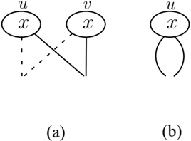
ABDDisreduced such that no pair of distinct nodes u and v are associated with the same variable and low and high successors (Fig. 3a), and no variable node u has identical low and high successors (Fig. 3b). Due to these reductions, the number of nodes

in a BDD for many functions encountered in practice is often much smaller than the number of truth assignments of the function. Another advantage is that the reductions make BDDs canonical [11]. Large space savings can be obtained by representing a collection of BDDs in a single multi-rooted graph where the sub-graphs of the BDDs are shared. Due to the canonicity, two BDDs are identical if and only if they have the same root. Consequently, when using this representation, equivalence checking between two BDDs can be done in constant time. In addition, BDDs are easy to manipulate. Any Boolean operation on two BDDs can be carried out in time proportional to the product of their size. The size of a BDD can depend critically on the variable ordering. To find an optimal ordering is a co-NP-complete problem in itself [11], but a good heuristic for choosing an ordering is to locate dependent variables close to each other in the ordering. For a comprehensive introduction to BDDs and branching programs in general, we refer the reader to Bryant's original paper [11] and the books [12,13].

3.2 Compiling the Configuration Model

Each of the finite domain variables x i with domain D i = { 0 , . . . , | D i | -1 } is encoded by k i = /ceilingleft log | D i |/ceilingright Boolean variables x i 0 , . . . , x i k i -1 . Each j ∈ D i , corresponds to a

binary encoding v 0 . . . v k i -1 denoted as v 0 . . . v k i -1 = enc ( j ) . Also, every combination of Boolean values v 0 . . . v k i -1 represents some integer j ≤ 2 k i -1 , denoted as j = dec ( v 0 . . . v k i -1 ) . Hence, atomic proposition x i = v is encoded as a Boolean expression x i 0 = v 0 ∧ . . . ∧ x i k i -1 = v k i -1 . In addition, domain constraints are added to forbid those assignments to v 0 . . . v k i -1 which do not translate to a value in D i , i.e. where dec ( v 0 . . . v k i -1 ) ≥ | D i | .

Let the solution space Sol over ordered set of variables x 0 < . . . < x k -1 be represented by a Binary Decision Diagram B ( V, E, X b , R, var ) , where V is the set of nodes u , E is the set of edges e and X b = { 0 , 1 , . . . , | X b | -1 } is an ordered set of variable indexes, labelling every non-terminal node u with var ( u ) ≤ | X b | -1 and labelling the terminal nodes T 0 , T 1 with index | X b | . Set of variable indexes X b is constructed by taking the union of Boolean encoding variables ⋃ n -1 i =0 { x i 0 , . . . , x i k i -1 } and ordering them in a natural layered way, i.e. x i 1 j 1 < x i 2 j 2 iff i 1 < i 2 or i 1 = i 2 and j 1 < j 2 .

Every directed edge e = ( u 1 , u 2 ) has a starting vertex u 1 = π 1 ( e ) and ending vertex u 2 = π 2 ( e ) . R denotes the root node of the BDD.

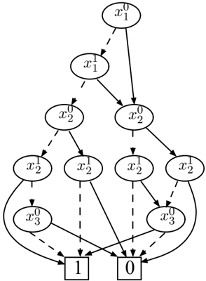
Example 2. The BDD representing the solution space of the T-shirt example introduced in Sect. 2 is shown in Fig. 4. In the T-shirt example there are three variables: x 1 , x 2 and x 3 , whose domain sizes are four, three and two, respectively. Each variable is represented by a vector of Boolean variables. In the figure the Boolean vector for the variable x i with domain D i is ( x 0 i , x 1 i , · · · x l i -1 i ) , where l i = /ceilingleft lg | D i |/ceilingright . For example, in the figure, variable x 2 which corresponds to the size of the T-shirt is represented by the Boolean vector ( x 0 2 , x 1 2 ) . In the BDD any path from the root node to the terminal node 1 , corresponds to one or more valid configurations. For example, the path from the root node to the terminal node 1 , with all the variables taking low values represents the valid configuration ( black , small , MIB ) . Another path with x 0 1 , x 1 1 , and x 0 2 taking low values, and x 1 2 taking high value represents two valid configurations: ( black , medium , MIB ) and ( black , medium , STW ) , namely. In this path the variable x 0 3 is a don't care variable and hence can take both low and high value, which leads to two valid configurations. Any path from the root node to the terminal node 0 corresponds to invalid configurations. ♦

4 Calculating Valid Domains

Before showing the algorithms, let us first introduce the appropriate notation. If an index k ∈ X b corresponds to the j + 1 -st Boolean variable x i j encoding the finite domain variable x i , we define var 1 ( k ) = i and var 2 ( k ) = j to be the appropriate mappings. Now, given the BDD B ( V, E, X b , R, var ) , V i denotes the set of all nodes u ∈ V that are labelled with a BDD variable encoding the finite domain variable x i , i.e. V i = { u ∈ V | var 1 ( u ) = i } . We think of V i as defining a layer in the BDD. We define In i to be the set of nodes u ∈ V i reachable by an edge originating from outside the V i layer, i.e. In i = { u ∈ V i | ∃ ( u ′ , u ) ∈ E. var 1 ( u ′ ) < i } . For the root node R , labelled with i 0 = var 1 ( R ) we define In i 0 = V i 0 = { R } .

We assume that in the previous user assignment, a user fixed a value for a finite domain variable x = v, x ∈ X , extending the old partial assignment ρ old to the current

assignment ρ = ρ old ∪ { ( x, v ) } . For every variable x i ∈ X , old valid domains are denoted as D ρ old i , i = 0 , . . . , n -1 . and the old BDD B ρ old is reduced to the restricted BDD, B ρ ( V, E, X b , var ) . The CVD functionality is to calculate valid domains D ρ i for remaining unassigned variables x i /negationslash∈ dom ( ρ ) by extracting values from the newly restricted BDD B ρ ( V, E, X b , var ) .

To simplify the following discussion, we will analyze the isolated execution of the CVD algorithms over a given BDD B ( V, E, X b , var ) . The task is to calculate valid domains V D i from the starting domains D i . The user-configurator interaction can be modelled as a sequence of these executions over restricted BDDs B ρ , where the valid domains are D ρ i and the starting domains are D ρ old i .

The CVD functionality is delivered by executing two algorithms presented in Fig. 5 and Fig. 6. The first algorithm is based on the key idea that if there is an edge e = ( u 1 , u 2 ) crossing over V j , i.e. var 1 ( u 1 ) < j < var 1 ( u 2 ) then we can include all the values from D j into a valid domain V D j ← D j .

We refer to e as a long edge of length var 1 ( u 2 ) -var 1 ( u 1 ) . Note that it skips var ( u 2 ) -var ( u 1 ) Boolean variables, and therefore compactly represents the part of a solution space of size 2 var ( u 2 ) -var ( u 1 ) .

For the remaining variables x i , whose valid domain was not copied by CVD -Skipped , we execute CVD ( B,x i ) from Fig. 6. There, for each value j in a domain D ′ i we check whether it can be part of the domain D i . The key idea is that if j ∈ D i then there must be u ∈ V i such that traversing the BDD from u with binary encoding of j

CVD -Skipped ( B ) 1: for each i = 0 to n -1 2: L [ i ] ← i +1 3: T ← TopologicalSort ( B ) 4: for each k = 0 to | T | -1 5: u 1 ← T [ k ] , i 1 ← var 1 ( u 1 ) 6: for each u 2 ∈ Adjacent [ u 1 ] 7: L [ i 1 ] ← max { L [ i 1 ] , var 1 ( u 2 ) } 8: S ←{} , s ← 0 9: for i = 0 to n -2 10: if i +1 < L [ s ] 11: L [ s ] ← max { L [ s ] , L [ i +1] } 12: else 13: if s +1 < L [ s ] S ← S ∪ { s } 14: s ← i +1 15: for each j ∈ S 16: for i = j to L [ j ] 17: V D i ← D i

/negationslash

CVD ( B,x i ) 1: V D i ←{} 2: for each j = 0 to | D i | -1 3: for each k = 0 to | In i | -1 4: u ← In i [ k ] 5: u ′ ← Traverse ( u,j ) 6: if u ′ = T 0 7: V D i ← V D i ∪{ j } 8: Return

will lead to a node other than T 0 , because then there is at least one satisfying path to T 1 allowing x i = j .

Traverse ( u,j ) 1: i ← var 1 ( u ) 2: v 0 , . . . , v k i -1 ← enc ( j ) 3: s ← var 2 ( u ) 4: if Marked [ u ] = j return T 0 5: Marked [ u ] ← j 6: while s ≤ k i -1 7: if var 1 ( u ) > i return u 8: if v s = 0 u ← low ( u ) 10: else u ← high ( u ) 12: if Marked [ u ] = j return T 0 13: Marked [ u ] ← j 14: s ← var 2 ( u )

When traversing with Traverse ( u, j ) we mark the already traversed nodes u t with j , Marked [ u t ] ← j and prevent processing them again in the future j -traversals Traverse ( u ′ , j ) . Namely, if Traverse ( u, j ) reached T 0 node through u t , then any other traversal Traverse ( u ′ , j ) reaching u t must as well end up in T 0 . Therefore, for every value j ∈ D i , every node u ∈ V i is traversed at most once, leading to worst case running time complexity of O ( | V i | · | D i | ) . Hence, the total running time for all variables is O ( ∑ n -1 i =0 | V i | · | D i | ) .

Thetotal worst-case running time for the two CV D algorithms is therefore O ( ∑ n -1 i =0 | V i |· | D i | + | E | + n ) = O ( ∑ n -1 i =0 | V i | · | D i | + n ) .

References

1. Jensen, R.M.: CLab: A C++ library for fast backtrack-free interactive product configuration. http://www.itu.dk/people/rmj/clab/ (2007)
2. Raskin, J.: The Humane Interface. Addison Wesley (2000)
3. Amilhastre, J., Fargier, H., Marquis, P.: Consistency restoration and explanations in dynamic CSPs-application to configuration. Artificial Intelligence 1-2 (2002) 199-234 ftp://fpt.irit.fr/pub/IRIT/RPDMP/Configuration/ .
4. Madsen, J.N.: Methods for interactive constraint satisfaction. Master's thesis, Department of Computer Science, University of Copenhagen (2003)
5. Hadzic, T., Subbarayan, S., Jensen, R.M., Andersen, H.R., Møller, J., Hulgaard, H.: Fast backtrack-free product configuration using a precompiled solution space representation. In: PETO Conference, DTU-tryk (2004) 131-138
6. Møller, J., Andersen, H.R., Hulgaard, H.: Product configu ration over the internet. In: Proceedings of the 6th INFORMS Conference on Information Systems and Technology. (2002)
7. Configit Software A/S. http://www.configit-software.com (online)

1. Tsang, E.: Foundations of Constraint Satisfaction. Academic Press (1993)
2. Dechter, R.: Constraint Processing. Morgan Kaufmann (2003)
3. Subbarayan, S., Jensen, R.M., Hadzic, T., Andersen, H.R., Hulgaard, H., Møller, J.: Comparing two implementations of a complete and backtrack-free interactive configurator. In: CP'04 CSPIA Workshop. (2004) 97-111
4. Bryant, R.E.: Graph-based algorithms for boolean function manipulation. IEEE Transactions on Computers 8 (1986) 677-691
5. Meinel, C., Theobald, T.: Algorithms and Data Structures in VLSI Design. Springer (1998)
6. Wegener, I.: Branching Programs and Binary Decision Diagrams. Society for Industrial and Applied Mathematics (SIAM) (2000)