Chain graphs for learning

Wray L. Buntine* RIACS at NASA Ames Research Center Mail Stop 269-2 Moffett Field, CA 94035-1000, USA wray�kronos.arc.nasa.gov

Abstract

Chain graphs combine directed and undi­ rected graphs and their underlying mathe­ matics combines properties of the two. This paper gives a simplified definition of chain graphs based on a hierarchical combination of Bayesian (directed) and Markov (undirected) networks. Examples of a chain graph are multivariate feed-forward networks, cluster­ ing with conditional interaction between vari­ ables, and forms of Bayes classifiers. Chain graphs are then extended using the notation of plates so that samples and data analysis problems can be represented in a graphical model as well. Implications for learning are discussed in the conclusion.

1 Introduction

Probabilistic networks are a notational device that allow one to abstract forms of probabilistic reason­ ing without getting lost in the mathematical detail of the underlying equations. They offer a framework whereby many forms of probabilistic reasoning can be combined and performed on probabilistic models with­ out careful hand programming. Efforts to date have largely focused on first-order probabilistic inference, for instance found in expert systems and diagnosis (Heckerman, Mamdani, & Wellman, 1995; Spiegelhal­ ter, Dawid, Lauritzen, & Cowell, 1993), and planning (Dean & Wellman, 1991). For instance, given a set of observations about a patient, what are the posterior probabilities for different diseases? Should an addi­ tional expensive diagnostic test be performed on the patient? This paper presents a representation for ex­ tending probabilistic networks to handle second-order or statistical problems. Second order problems are mainly concerned with building or improving a proba­ bilistic network from a database of cases. Second order

*Current address: Heuristicrats Research, Inc., 1678 Shattuck Avenue, Suite 310, Berkeley, CA 94709-1631, wrayGHeuristicrat.COM

inference on probabilistic networks was first suggested by Lauritzen and Spiegelhalter (Lauritzen & Spiegel­ halter, 1988), and has subsequently been developed by several groups {Gilks, Thomas, & Spiegelhalter, 1993; Dawid & Lauritzen, 1993; Buntine, 1994; Shachter, Eddy, & Hasselblad, 1990). Whereas, an introduc­ tion to learning of Bayesian networks can be found in (Heckerman, 1995).

This paper uses chain graphs (Lauritzen & Wermuth, 1989) as a general probabilistic network model. Chain graphs mix undirected and directed graphs (or net­ works) to give a probabilistic representation that in­ cludes Markov random fields and various Markov models. Lauritzen and Wermuth demonstrated that chain graphs are a powerful tool for modeling statis­ tical analysis, research hypotheses, and hence learn­ ing (Wermuth & Lauritzen, 1989). Chain graphs when augmented with deterministic nodes can repre­ sent many well known models as a special case includ­ ing generalized linear models, various forms of cluster­ ing, feed-forward neural networks and various stochas­ tic neural networks. This includes a large number of the more general network models now available (Rip­ ley, 1994). These many different models are formed by combining basic nodes in the network represent­ ing for instance, Gaussian variables or deterministic Sigmoid units. The expressiveness of chain graphs is illustrated in Section 6 where a number of models are represented. Decision theoretic constructs could also be used to represent the decisions and utilities of a problem {Shachter, 1986), although this is not done here.

In this paper, I define a chain graph as a hierarchi­ cal combination of directed (Bayesian) and undirected (Markov) networks. This definition extends the no­ tion of block recursive models used in (Wermuth & Lauritzen, 1989; H¢jsgaard & Thiesson, 1995) and analyzed in (Frydenberg, 1990, Theorem 4.1) by al­ lowing blocks to include directed networks as well as undirected networks. This definition allows the com­ plex independence properties and functional form of a chain graph (Frydenberg, 1990) to be read off from knowledge of the simpler corresponding properties for directed and undirected networks. This definition also

allows chain graphs to have embedded deterministic nodes-as commonly used in learning for neural net­ works, generalized linear models, and basis functions­ and thus extends the general applicability of chain graphs. Previous constructions relied on positivity constraints (Frydenberg, 1990) so did not allow deter­ minism, or used limit theorems (H¢jsgaard & Thies­ son, 1995) to allow some determinism. This framework for modeling chain graphs, and the general interpre­ tation theorem, Theorem 2, are the major technical contribution of this paper.

First, Sections 2 and 3 review basic results on directed and undirected networks, as for instance introduced in (Pearl, 1988; Whittaker, 1990). Necessary inde­ pendence properties and functional representations of these networks, as needed for chain graphs, are sum­ marized. Then the notion of conditional networks are formalized in Section 4. Conditional networks are im­ plicitly used throughout the community, however we need to define them carefully as a building block for the definition of chain graphs. A chain graph is then introduced as a hierarchical combination of conditional networks, in Section 5. Several examples of learning systems are then given. Finally, a graphical construct for modeling samples and learning, plates (Buntine, 1994), is reviewed.

2 Directed networks

A Bayesian or directed network consists of a set of variables X and a directed graph defined on it consist­ ing of a node corresponding to each variable and a set of directed arcs. Nodes in the graph and the variables they represent are used interchangeably. The graph is such that it contains no directed cycles. In this paper, a directed network defines a particular func­ tional form for the probability distribution p(X) over the variables. Each variable is written conditioned on its parents, where parents( :z:) is the set of variables with a directed arc into :z:. The general form for this equation for a set of variables X is:

This functional form is the interpretation of a directed network used in this paper. The lemma below shows that this definition is equivalent to a definition based in independence statements (Lauritzen, Dawid, Larsen, & Leimer, 1990), related to (Pearl, 1988). The inde­ pendence notation is due to (Dawid, 1979).

Definition 1 A is independent of B given C, denoted AllBIC, when p(A U BIG) = p(AIC)p(BIC) for all instantiations of the variables A, B, C.

The following definitions are used here.

Definition 2 The ancestral set, ancestors(A), of a subset A of variables X is the transitive closure of the relation, f(B) = B U parents( B). The moralized graph Gm of a directed graph G is formed by connect­ ing every two nodes that have a common child with an undirected arc, and then dropping the directions from all directed arcs.

The particular independence statements are based on set separation in the moralized graph, which is equivalent to another condition known as d-separation (Pearl, 1988):

Definition 3 The distribution p(X) satisfies the di­ rected global Markov property relative to the directed graph G if AliBIS when S separates A and B in the graph Hm where H is the subgraph of G restricted to ancestors( A U B U S) .

Lemma 1 Given a directed graph G on X, and A, B, S E X. The distribution p(X) satisfies the di­ rected global Markov property relative to G if and only if Equation {1} holds.

Given a directed graph, we can therefore read off both the functional decomposition of Equation (1) and the independence properties easily.

3 Undirected networks

Similarly, a Markov or undirected network is an undi­ rected graph on a set of variables X representing a probability distribution p(X) over the variables. This is analogous to Lemma 1, except that p(X) must now be strictly positive. The appropriate independence conditions are based on set separation without first moralizing the graph.

Definition 4 The distribution p(X) satisfies the global Markov property relative to the undirected graph G if AllB IS when S separates A and B in the graph G.

The neighbors for a node :z:, denoted neighbors(:z:) are the set of variables directly connected by an undirected arc to :z:. An important concept is the set of cliques on the graph.

Definition 5 The set of maximal cliques on G is de­ noted Cliques( G) C 2 x . C E Cliques( G) if and only if C is fully connected in G and no strict superset of C is fully connected in G.

Theorem 1 An undirected graph G is on variables in the set X. The distribution p(X) is strictly positive in the domain X x E x domain( :z:). Then the distribution p(X) satisfies the global Markov property if and only if p(X) satisfies the equation

for some functions f c > 0.

The proof follows directly from ( Frydenberg, 1990; Buntine, 1994). A form of this theorem for finite dis­ crete domains is called the Hammersley-Clifford The­ orem ( Geman, 1990; Besag, York, & Mollie, 1991). Again, Equation (2) is used as the interpretation of an undirected network.

4 Conditional networks

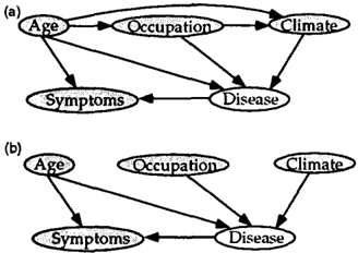
Networks can also represent conditional probabil­ ity distributions. Conditional networks are repre­ sented by introducing shaded variables in the graph. Shaded variables are assumed to have their values known, so the probability defined by the network is now conditional on the shaded variables. Fig­ ure 1 shows two conditional versions of a simple med­ ical problem ( Shachter & Heckerman, 1987). If the

shading of nodes is ignored, the joint probability, p(Age, Occ, Clim, Dis, Symp) for the two graphs ( a ) and ( b ) respectively is:

• (a) p(Age) p(OcciAge)p(ClimiAge, Occ) p(DisiAge, Occ,
• (b) p(SympiAge, Dis)

However, because four of the five nodes are shaded, this means their values are known. The conditional distributions computed from the above are identical:

p(DisiAge, Occ, Clim, Symp)

More generally, conditional networks can be simpli­ fied sometimes ( Buntine, 1994 ) . The following simple lemma applies to conditional Bayesian networks and is derived directly from Equation ( 1 ) .

Lemma 2 Given a directed network G with some nodes shaded representing a conditional probability dis­ tribution. If a node X and all its parents have their values given, then the Bayesian network G' created by deleting all the arcs into X represents an equivalent probability model to the Bayesian network G.

A corresponding result holds for undirected graphs, and follows directly from Theorem 1.

Lemma 3 Given an undirected graph G with some nodes shaded representing a conditional probability dis­ tribution. Delete an arc between given nodes A and B if all their common neighbors are given. The resultant graph G' represents an equivalent probability model to the graph G.

Furthermore, the probability formula for conditional networks follow easily as well from the corresponding Equations ( 1 ) and (2).

Lemma 4 Let G be a conditional directed graph on variables X U Y where variables Y are given and X are not. Then if Y =ancestors(¥),

If G is a conditional undirected graph, then

for some function fy on Y.

Again, Equations (3) and (4) are used as the inter­ pretation of conditional undirected network, and the marginal distribution for the shaded variables, p(Y), is ignored. Furthermore, independence statements de­ rived from the graph are only valid if they are condi­ tioned on the shaded variables Y.

5 Chain graphs

A chain graph is a graph consisting of mixed directed and undirected arcs, where any cycle with some di­ rected arcs must contain at least two directed arcs in reverse direction. It is shown below that a chain graph can be represented as a hierarchical combination of conditional networks. A chain graph is first broken up into components as follows. The chain components are the standard definition used ( Lauritzen & Wermuth, 1989).

Definition 6 Given a chain graph G over some vari­ ables X. The chain components are the coarsest mutu­ ally e:z:clusive and e:z:haustive partition of X where the set of subgraphs induced by the partition are connected and undirected. Let chain-components(A) denote all nodes in the same chain component as at least one variable in A.

The chain components are unique and are found by re­ moving the directed arcs from the graph G and identi­ fying the connected components on the resulting graph ( Lauritzen & Wermuth, 1989 ) .

Definition 7 Given a chain graph G over some vari­ ables X. The component subgraphs are a coarser par­ tition of variables X than the chain components, and

are the coarsest partition where the set of subgraphs induced by the partition are connected, undirected or directed (but not mixed) subgraphs of the chain graph G.

These definitions imply that:

• a connected directed network has only a single component subgraph, itself; and
• likewise a connected undirected network has only a single component subgraph, itself.

This makes the component subgraphs a natural de­ composition of the chain graph into its maximal di­ rected and undirected parts. The following lemma shows the component subgraphs are unique.

Lemma 5 There is a unique set of component sub­ graphs for a chain graph G found by the following al­ gorithm:

Let U be the set of chain components for graph G, and letS be the set of singleton sets in U. Let D be the connected components in the graph G s (the graph G restricted to the variables in S, which is directed by construc­ tion). The component subgraphs are given by (U-S) U D and the subgraphs they induce.

Proof A component subgraph that is directed cannot contain two variables connected by an undirected arc. Furthermore, it is a superset of one or more chain com­ ponents since component subgraphs are by definition a coarser partition than the chain components. There­ fore, the component subgraphs that are directed must be formed by merging singleton chain components that are connected by directed arcs. This is the connectiv­ ity relation which has a unique coarsest partition. The algorithm above follows from this. D

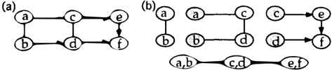
An example is given in Figure 2. Figure 2 ( a ) shows

the original chain graph. The chain components of G are {a, b}, {c}, {d}, and {e, f, g, h}. The compo­ nent subgraphs are formed by merging c and d into a directed graph on c, d. Figure 2 ( b ) shows on the left the three directed and undirected component sub­ graphs with their parents added and shaded. On the right is the Bayesian network showing how the compo­ nent subgraphs are pieced together. Theorem 2 below shows this leads to the following functional form for the joint probability.

Notice that f0(b, c) exists to normalize p(e, f, g, hlb, c).

Informally, a chain graph over variables X with com­ ponent subgraphs given by the set Tis interpreted first as the component factorization ( compared to a block factorization ( H!11jsgaard & Thiesson, 1995)) given by:

where

and likewise for ancestors. The conditional probabil­ ity p(rlparents(r)) for each component subgraph is now defined as a conditional directed or undirected network.

This can be formalized to give a definition for the in­ terpretation of a chain graph. This works through the steps given for interpreting Figure 2.

Definition 8 Given a chain graph G on variables X with no given nodes. Let U1, ... , U c be the component subgraphs of G. Construct a matching set of subgraphs G1, ... , Gc as follows. Let G; be the subgraph induced by G on U; U parents( U;). Then, make the variables in parents(U;) all be shaded in G; and add e:z:tra arcs to make parents(U;) into a clique. The e:z:tra arcs should be directed if U; is a directed component subgraph, and undirected if U; is undirected. Now construct a directed graph GM whose nodes are U 1 , . · · , Uc and arcs con­ nect U; to Uj if a variable in U; has a child in Uj in the graph G. Then the chain graph G is defined to be equivalent to the set of subgraphs G1, ... , Gc together with the master graph G M .

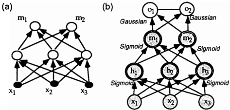
The subgraphs G; can also be simplified according to Lemmas 2 and 3. One advantage of this for­ mulation is that only undirected subcomponents of the chain graph need have the condition of positiv­ ity on their conditional distribution, required for The­ orem 1 to hold. An additional example of Defini­ tion 8 appears in Figure 3. The original chain graph is in Figure 3 ( a ) . In this case, the chain compo­ nents are { {a, b} , { c, d} , { e} , {I} }. The component subgraphs are { {a, b} , { c, d} , { e, ! } }. The graphs G1, G"J, G3 are shown in Figure 3 ( b ) along with the master graph Gm. The joint probability, whose gen­ eral form is derived below, is

�

Figure 3: Decomposing another chain graph

The global Markov property for chain graphs is defined in the same way as the directed global Markov prop­ erty. This requires that a chain graph be moralized. The definition below describes how this is done.

Definition 9 The ancestral set, ancestors(A), of a subset A of variables X is the transitive closure of the relation, f (B) = B U neighbors( B) U parents(B). The moralized graph em of a chain graph G is formed by connecting every two nodes that have children in a common chain component with an undirected arc, and then dropping the directions from all directed arcs.

The corresponding relationship between independence and the functional form of the probability distribution then follows from Lemma 1 and Theorem 1, although not trivially so.

Theorem 2 A chain graph G is on variables in the set X. For every U C X a chain component of G with cardinality greater than 1, the conditional distri­ bution p(Uiparents(U)) is strictly positive in the do­ main XxEudomain(:z:). Then the distribution p(X) satisfies the global Markov property if and only if p(X) satisfies Equations {3) and {4) for each of its subgraphs and master graphs.

Proof The proof uses the notation from Definition 8. First, assume the joint probability p(X) satisfies Equa­ tions (3) and ( 4) as required for the component sub­ graphs and the master graph, and prove the global Markov property holds. The joint probability there­ fore satisfies Equation (5) where T is the set of com­ ponent subgraphs and the terms p(rlparents(r)) are given by Equations (3) and ( 4). Since the directed component subgraphs satisfy Equations (3), it follows that

where T' are the chain components. Consider testing whether AllB I D. Let Z = ancestors( A U B U D). By construction, the marginal distribution for Z is a restriction of this product to the chain components for z.

where again the terms p(rlparents(r)) are given by Equation ( 4) for T non-singleton. Let G'£ be the mor­ alized version of the chain graph G restricted to Z. Since the moralized graph joins parents with an undi- rected arc, p( Z) takes the form of

Now assume D separates A and B in Z. The follow­ ing shows AllB I D. Due to separation, if we remove variables in D from G'£, the resulting graph separates into a part containing A, ZA, and a part containing B, ZB, where AnZB = 0 = BnZA. Ignoring variables in D, each clique in G'£ must be wholly contained in one part or another. Hence, p(Z) = fi(ZA, D) h(ZB, D), and therefore independence holds by marginalizing out variables in Z-A-B-D.

Now for the reverse direction. Assume the global Markov property holds. Equation (5) follows directly. Now apply the global Markov property to each of the subgraphs G; in Definition 8. Suppose G; is directed. Let :z: � U;. Since :z: has no neighbors in G, it follows from the global Markov property for the chain graph that :z:llancestors(:z:) jparents(:z:). Notice that ances­ tors in G; are a subset of the ancestors in G so Equa­ tion (3) follows. Suppose G; is undirected. The condi­ tion in the theorem implies that p(U;jparents(Ui)) is strictly positive in the domain XxEUdomain(:z:). Also, the global Markov property implies that for :z: E U;, :z:ll(U;Uparents(Ui)) I (neigbors(:z:)Uparents(:z:)). Us­ ing a proof like that for (Buntine, 1994, Theorem 2.1), Equation ( 4) follows. 0

A number of interesting properties can be derived from the global Markov property for chain graphs, their equivalence, and their relationship with Bayesian networks (Frydenberg, 1990; Andersson, Madigan, & Perlman, 1994). For instance, a chain graph is a convenient representation for the class of equivalent Bayesian networks (Verma & Pearl, 1990).

6 Examples of chain graphs for learning

This section presents a number of models using chain graphs, to illustrate their generality.

6.1 Feed-forward networks and deterministic nodes

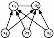
The preceding definitions of a chain graph have been carefully set up to allow nodes to represent determin­ istic variables. Consider a feed-forward network, pop­ ular in neural networks, and general enough to repre­ sent logistic or linear regression. A simple feed-forward network is given in Figure 4(a). The corresponding chain graph is given in Figure 4(b), which also intro­ duces a bivariate Gaussian error model on the output variables. Here the five sigmoid units of the network are modeled with deterministic nodes. A deterministic node has double circles to indicate it is a deterministic function of its inputs. The analysis of deterministic nodes in Bayesian networks and, more generally, in

influence diagrams is considered by { Shachter, 1990). The network outputs m1 and m2 represent the mean of a bivariate Gaussian.

To analyze these nodes, we need to extend the usual definition of a parent and a child for a graph. Only one case is given here because it is all that is used in the lemma below.

Definition 10 The non-deterministic children of a node :z: are the set of non-deterministic variables y such that there exists a directed path from :z: to y given by :z:, Yl! ... , Yn1 y, with all intermediate variables (Yt, ... , Yn) being deterministic.

For instance, in the model in Figure 4, the non­ deterministic children of z:� are o1 and o2· Determin­ istic nodes can be removed from a graph by rewriting the equations represented into the remaining variables of the graph. This goes as follows:

Lemma 6 A chain graph G with nodes X has deter­ ministic nodes Y C X. The chain graph G' is created by adding to G a directed arc from every node to its non-deterministic children, and by deleting the deter­ ministic nodes Y. The graphs G and G' are equivalent probability models on the nodes X -Y.

An application of this lemma to the chain graph in Figure 4 is given in Figure 5. This of course, destroys

all the information conveyed by the original graph.

6.2 Stochastic neural networks

Stochastic networks form the basis of the stochastic Boltzmann machine, and the Hopfield network ( Hertz,

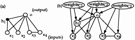
Krogh, & Palmer, 1991), which both have relation­ ships to graphical models ( Neal, 1992). A stochastic network corresponds to an undirected network with hidden variables, except interactions involve quadratic terms at most. A simple configuration is given in Fig­ ure 6. On the left is a representation of a network

for a Boltzmann using the notation in ( Hertz et al., 1991). The input variables are :z: 1 , :z:2, :z:3 and :z:4 and the output variable is o. There is one hidden variable h1 marked in black. The corresponding chain graph is on the right with the parameters for the model, the weights, explicitly represented. The weights of the feed-forward network were not represented in the ex­ ample of the previous section. This chain graph has four chain components.

These components also correspond to the component subgraphs. The fourth and largest component sub­ graph when extended with its parents, as required for Definition 8, corresponds to the entire Figure 6 ( b ) but with the directions of the arcs dropped. The cliques in this component subgraph with parents included are:

From Equations {3) and {4) it follows that the condi­ tional probability is given by:

where the normalizing constant would be determined. Notice the terms p( weights c.) have been dropped from this expression because they normalize out. Since the variable h1 is hidden, and the target is the prob­ ability of the output o, the conditional probability p(oizt, :z:2, :z:3, :z:4, weights) would be found via Bayes theorem.

where again the normalizing constant is to be deter­ mined. As this stands, this allows the functions fc,,

f c , and /c, to take on a general form so this is re­ ally a higher-order Boltzmann machine. Boltzmann machines traditionally only involve quadratic terms. The correspondence between stochastic neural net­ works and probabilistic networks is not exact.

6.3 Bayesian classifiers

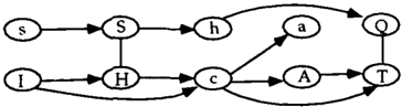
Bayesian classifiers ( Duda & Hart, 1973) are a broad family of supervised learning systems. Bayesian net­ works offer a rich representation for designing many different kinds of Bayesian classifiers, for instance illus­ trated with the Bayesian conditional trees of ( Geiger, 1992). Chain graphs offer a richer family again of Bayesian classifiers, and a nice framework for their elicitation. During elicitation we can interpret the di­ rected arcs in the "true" 1 chain graph as being causal connections, and undirected arcs as being associational connections. The language of chain graphs allow as­ sociations to be represented in a model in those situa­ tions where causality is perhaps difficult to interpret. This is illustrated by ( H!11jsgaard & Thiesson, 1995). They present an example where a Bayesian classifier for Coronary artery disease is constructed by learn­ ing a chain graph from data, and then conditioning the chain graph for the key target variable Coronary artery di6ease, denoted c using the formula

where other-vars is the other variables in the graph. Prior information about the underlying "true" chain graph is elicited from a clinician. This prior informa­ tion represents constraints on the eventual chain com­ ponents, and directed and undirected arcs which defi­ nitely should or should not be present. The clinician's prior includes such constraints as ( the corresponding variable in the graph follows in brackets ) :

• sex (s) is a causal factor for smoking (S),
• there is no association between previous myocar­ dial infarct (A) and angina pectoris (a),
• there is possible association between EGG­ examinations Q-wave ( Q) and T-wave (T) but there is no causal link between the two.

A sample chain graph consistent with this prior knowl­ edge is given in Figure 7 ( this simplifies the situation presented in ( H!11jsgaard & Thiesson, 1995)).

7 Chain graphs with plates

To represent data analysis problems within a network language such as chain graphs, some additions are

1 The terms "true model", "causal", and "associations" used here are controversial so consider them to be fictions introduced for the purposes of elicitation.

needed. As a notational device to represent a sample­ a group of like variables whose conditional distribu­ tions are independent and identical-plates are used on a chain graph ( Buntine, 1994). By defining var­ ious operations on chain graphs with plates, such as conditioning and differentiation, useful algorithms can be pieced together for standard statistical procedures such as maximum likelihood or maximum a posteri­ ori calculations, or the expectation maximization al­ gorithm. Chain graphs with plates therefore represent a specification language for data analysis problems.

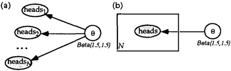
To introduce plates, consider the simplified version possible of a learning problem: there is a biased coin with an unknown bias for heads 9. That is, the long-

run frequency of getting heads for this coin on a fair toss is 9. The coin is tossed N times and each time the binary variable heads; is recorded. The graphical model for this is in Figure 8 ( a ) . The heads; nodes are shaded because their values are given, but the 9 node is not. The 9 node has a Beta(1.5, 1.5) prior. The data for this problem is the sequence of heads variables. The key thing to notice is that for an "in­ dependently and identically distributed" sample, the network model for each case will be equivalent, and will be conditioned on the same model parameter, 9. So the portion of the network corresponding to each i.i.d. case will be identical. Plates allow this duplica­ tion to be removed. The corresponding plate model for Figure 8 ( a ) is given in Figure 8 ( b ) .

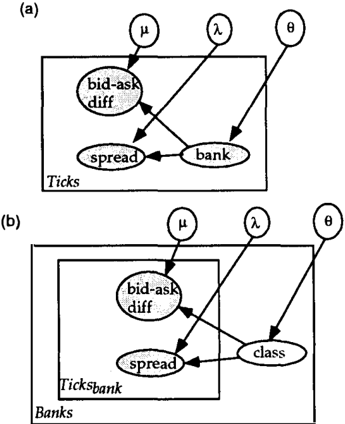
There can be multiple plates in the one diagram, in­ dicating multiple tables in the data set. Data for the dollar-Deutsch mark exchange rate consists of a se­ quence of bids posted by banks. Original data takes the form of a date and time, the bid and asking price, and the bank code. This is converted into the mean bid-ask price, (bid+ask)/2, and the spread, (ask-bid) because these variables more naturally representation the domain.

	Date	Mean bid-ask	Spread	Bank
Sep	1 13:42:40	1.57395	0.0005	CONY
Sep	1 13:42:45	1.5740	0.0010	MGTX
Sep	1 13:43:14	1.57375	0.0005	BBIX

The skeptic would say that price differences are ran­ dom and do not reflect any intelligent behavior by .the banks. The skeptic therefore models this data as a random walk. It is clear that individual banks be­ have differently, so one way to do this is to have a separate random walk for each bank. This is shown in Figure 9 { a ) where each row in the data above cor­ responds to one instance of the plate. The variable bid-a8k-diff is the difference in the mean bid-ask price from the bank's previous posting, which is random un­ der a random walk model. Another model is to group banks into separate classes, where random walks now occur for the prices in each class of banks. Of course, we do not know what these classes are ahead of time, so this is a new kind of unsupervised learning prob­ lem. A probabilistic network for this second model is shown in Figure 9 ( b ) . In this model, the bid-a8k-diffis

assumed to be influence by the class, but is otherwise random. Notice in this model the outer plate is index by the bank, so each instance represents a different bank. The variable Banks is the number of banks. The inner plate is indexed by a single bank's prices, so each instance represents a different price for that bank. The variable Ticksb,mk is the number of prices posted for the bank. This represents another view of the data set, where we have a table of banks with an inner table of prices for each bank.

Bank CONY

	Date	Mean bid-ask	Spread
Sep	1 13:42:40	1.57395	0.0005
Sep	1 13:42:45	1.5740	0.0010

The joint probability for the model of Figure 9 ( b ) is given by

p(spread;,j I>., class;) p(bid-a8k-diffi ,j IJ-L, class;) .

In this expression, Banks is an index set for the banks and Prices( i) is an index set for the prices for bank i. The product terms in the formula mirror the structure of the graph.

The notion of a plate is formalized below.

Definition 11 A chain graph G with plate8 on vari­ able 8et X consi8t8 of a chain graph G' on variable$ X with additional bo:ce8 called plate8 placed around group8 of variable$, Directed arc8 can only crou into plate81 undirected arc8 cannot crou plate boundarie8, and plate8 can be overlapping. Each plate P ha8 an in­ teger N p in the bottom left corner indicating ib cardi­ nality. The plate P inde:ce8 the variable8 in8ide it with value8 i = 1, . . . , N p . Each variable V E X occur8 in 8ome 8ubset of the plate8. Let indval(V) denote the 8et of value8 for indice8 corre8ponding to the8e plate8. That i81 indval(V) i8 the crou product of inde:c 8ets { 1, . . . , N p } for plate8 P containing V.

A graph with plates can be e:cpanded to remove the plates and replace them with the contents duplicated. Figure 8 ( a ) is an expanded form of Figure 8 ( b ) . This is done by duplicating the contents of the plate Np times, starting from the outermost plate and working inwards. The probability formula corresponding to a graph with plates can be written down from this ex­ panded form, as was done for Figure 9 ( b ) above. The details are tedious so I do not reproduce them here.

8 Conclusion

With chain graphs defined and operating for a large family of data analysis models in machine learning, neural networks and statistics, it is possible to crank the handle-apply the standard algorithmic methods for addressing probability problems-to create learn­ ing algorithm from the particular chain graph rep­ resentation. Some examples of papers that discuss general methods for learning on graphical models are ( Buntine, 1994; Gilks et al., 1993; Lauritzen, 1995 ) .

Acknowledgments

This paper was considerably improved by the sugges­ tions from the reviewers.

References

• Andersson, S., Madigan, D., & Perlman, M. (1994). On the Markov equivalence of chain graphs, undirected graphs, and acyclic digraphs. Techni­ cal report #281, Department of Statistics, Uni­ versity of Washington, Seattle, WA.
• Besag, J., York, J., & Mollie, A. (1991). Bayesian im­ age restoration with two applications in spatial statistics. Ann. Inst. Statist. Math., 43 (1) , 1-59.
• Buntine, W. (1994). Operations for learning with graphical models. Journal of Artificial Intelli­ gence Research, 2, 159-225.
• Dawid, A. ( 1979). Conditional independence in statis­ tical theory. SIAM Journal on Computing, 41, 1-31.
• Dawid, A., & Lauritzen, S. (1993). Hyper Markov laws in the statistical analysis of decomposable graphical models. Annals of Statistics, 2 1 (3), 1272-1317.
• Dean, T., & Wellman, M. ( 1991). Planning and Con­ trol. Morgan Kaufmann, San Mateo, California.
• Duda, R., & Hart, P. ( 1973). Pattern Classification and Scene Analysis. John Wiley, New York.
• Frydenberg, M. ( 1990). The chain graph Markov prop­ erty. Scandinavian Journal of Statistics, 17, 333353.
• Geiger, D. (1992). An entropy-based learning algo­ rithm of Bayesian conditional trees. In Dubois, D., Wellman, M., D'Ambrosio, B., & Smets, P. ( Eds. ) , Uncertainty in Artificial Intelligence: Proceedings of the Eight Conference, pp. 92-97 Stanford, CA.
• Geman, D. ( 1990). Random fields and inverse prob­ lems in imaging. In Hennequin, P. ( Ed. ) , E cole d' E te de Probabilites de Saint-Flour XVIII -1988. Springer-Verlag, Berlin. In Lecture Notes in Mathematics, Volume 1427.
• Gilks, W., Thomas, A., & Spiegelhalter, D. (1993). A language and program for complex Bayesian modelling. The Statistician, 43, 169-178.
• Heckerman, D. ( 1995). Bayesian networks for knowl­ edge representation and learning. In Fayyad, U. M., Piatetsky-Shapiro, G., Smyth, P., & Uthurasamy, R. S. ( Eds. ) , Advances in Knowl­ edge Discovery and Data Mining. MIT Press.
• Heckerman, D., Mamdani, A., & Wellman, M. (1995). Real-world applications of Bayesian networks: Introduction. Communications of the A CM, 38(3).
• Hertz, J., Krogh, A., & Palmer, R. (1991). Intro­ duction to the Theory of Neural Computation. Addison-Wesley.
• H¢jsgaard, S., & Thiesson, B. (1995). BIFROST Block recursive models Induced From Relevant
• knowledge, Observations, and Statistical Tech­ niques. Computational Statistics and Data Anal­ ysis, 19 (2) , 155-175.
• Lauritzen, S., & Wermuth, N. ( 1989). Graphical mod­ els for associations between variables, some of which are qualitative and some quantitative. An­ nals of Statistics, 17, 31-57.
• Lauritzen, S. (1995). The EM algorithm for graphi­ cal association models with missing data. Com­ putational Statistics and Data Analysis, 19 {2) , 191-201.
• Lauritzen, S., Dawid, A., Larsen, B., & Leimer, H.­ G. ( 1990). Independence properties of directed Markov fields. Networks, 20, 491-505.
• Lauritzen, S., & Spiegelhalter, D. (1988). Local com­ putations with probabilities on graphical struc­ tures and their application to expert systems ( with discussion ) . Journal of the Royal Statis­ tical Society B, 50(2), 240-265.
• Neal, R. (1992). Connectionist learning of belief net­ works. Artificial Intelligence, 56, 71-113.
• Pearl, J. (1988). Probabilistic Reasoning in Intelligent Systems. Morgan Kaufmann.
• Ripley, B. (1994). Network methods in statistics. In Kelly, F. ( Ed. ) , Probability, Statistics and Opti­ mization, pp. 241-253. Wiley & Sons, New York.
• Shachter, R. (1986). Evaluating influence diagrams. Operations Research, 34 (6) , 871-882.
• Shachter, R. (1990). An ordered examination of influ­ ence diagrams. Networks, 20, 535-563.
• Shachter, R., Eddy, D., & Hasselblad, V. (1990). An influence diagram approach to medical technol­ ogy assessment. In Oliver, R., & Smith, J. ( Eds. ) , Influence Diagrams, Belief Nets and Decision Analysis, pp. 321-350. Wiley.
• Shachter, R., & Heckerman, D. (1987). Thinking back­ wards for knowledge acquisition. AI Magazine, 8 ( Fall ) , 55-61.
• Spiegelhalter, D., Dawid, A., Lauritzen, S., & Cowell, R. (1993). Bayesian analysis in expert systems. Statistical Science, 8(3), 219-283.
• Verma, T., & Pearl, J. (1990). Equivalence and syn­ thesis of causal models. In Bonissone, P. ( Ed. ) , Proceedings of the Sixth Conference on Uncer­ tainty in Artificial Intelligence Cambridge, Mas­ sachusetts.
• Wermuth, N., & Lauritzen, S. (1989). On substantive research hypotheses, conditional independence graphs and graphical chain models. Journal of the Royal Statistical Society B, 51 (3).
• Whittaker, J. (1990). Graphical Models in Applied Multivariate Statistics. Wiley.