Confidence Inference in Bayesian Networks

Jian Cheng & Marek J. Druzdzel*

School of Information Sciences and Intelligent Systems Program

Decision Systems Laboratory University of Pittsburgh, Pittsburgh, PA 15260 {jcheng,marek}�sis.pitt.edu

Abstract

We present two sampling algorithms for prob­ abilistic confidence inference in Bayesian net­ works. These two algorithms (we call them AIS-BN-p and AIS-BN-li algorithms) guar­ antee that estimates of posterior probabilities are with a given probability within a desired precision bound. Our algorithms are based on recent advances in sampling algorithms for (1) estimating the mean of bounded random variables and (2) adaptive importance sam­ p li n g in Bayesian networks. In addition to a simple stopping rule for sampling that they provide, the AIS-BN-p and AIS-BN-0' al­ gorithms are capable of guiding the learning process in the AIS-BN algorithm. An em­ pirical evaluation of the proposed algorithms shows excellent performance, even for very unlikely evidence.

1 Introduction

The main application of stochastic sampling algo­ rithms in Bayesian networks is inference in very large networks in which exact methods are intractable. Stochastic sampling algorithms essentially trade off precision for computation sample generation can be interrupted at any time yielding an approximate answer. While absolute precision is seldom critical, it is often useful to know roughly how close the answer is to the exact answer or, in other words, what is the confidence interval around the computed result.

The best existing algorithms that address this problem a r e the bounded variance algorithm [Dagum and Luby, 1997] and the AA algorithm [Dagum et al., 2000]. The

Currently with ReasonEdge Technologies, Pte, Ltd, 438 Alexandra Road, #03-0lA Alexandra Point, Singapore 119958, Republic of Singapore, [email protected].

test results reported in Pradhan and Dagum [1996] show that these algorithms work well when the prob­ ability of evidence is not too small. However, as sim­ p le tests that we conducted showed, in very l a r ge net­ works, especially when several observations have been made and the probability of evidence is very small, these algorithms usually require a prohibitive number of samples to satisfy the requirement. One of the rea­ sons for this is that these algorithms are based on the likelihood weighting algorithm [Fung and Chang, 1989, Shachter and Peat, 1989], which suffers from the prob­ lem of mismatch between the optimal and the actually used importance function (see [Cheng and Druzdzel, 2000] for an in-depth discussion of this problem). An­ other problem is that the confidence intervals calcu­ lated by these algorithms are not tight enough. Re­ cent advances in simulation algorithms, notably the AIS-BN algorithm [Cheng and Druzdzel, 2000] and stopping rules [Cheng, 2001], address both of these problems.

In this paper, we combine the AIS-BN simulation al­ gorithm with the new stopping rules to yield two sam­ pling algorithms that perform well in very large net­ works. Essentially, our approach is to use the new stopping rules in the AIS-BN algorithm to guide the process of learning the importance function. After each learning step, we use the SA-Jl or SA-li algo­ rithm [ Cheng, 2001] to produce the estimated number of samples that is needed to achieve a required pre­ cision. SA-p and SA-a algorithms are currently the best known distribution-independent algorithms to es­ timate the mean and they require a relatively small number of samples. In addition to estimating the num­ ber of samples needed to achieve a desired precision, the resulting AIS-BN-p and AIS-BN-a algorithms re­ act to situations when the number of samples is pro­ hibitive. In our approach, the a lgo r i t h m s use heuristic methods to modify the importance function combined with a restart, whereby typically the second try solves the problem of prohibitive computation.

In the following discussion, capital letters, such as A, B, or C will denote multiple-valued, discrete random variables. Bold capital l e tte r s , such as A, B, or C, denote sets of variables. E will denotes the set of evidence variables. Lower case letters a, b, c denote particular instantiations of variables A, B, and C re­ spectively. Bold lower case letters, such as a, b, c, and e, denote particular instantiations o f A, B, C, and E respectively. Pa(A) denotes the parents of node A. Pr( X ) denotes the network joint probability distribu­ tion. \ de no t e s set difference. Vertical bar, such as in P a(A)\ E ==e' denotes substitution of e forE in A. w(k) or Pr(k) denote a number or a function in stage k.

2 AIS-BN: Adaptive Importance Sampling for Bayesian Networks

Because familiarity with the AIS-BN alg o r i t h m will be helpful in understanding the current paper, we will briefly review its design. Readers interested in details are directed to the exposition in [Cheng and Druzdzel, 2000].

The AIS-BN a lg o r i thm is based on importance sam­ pling in finite dimensional integrals. Using the struc­ tural advantages of B ay es i an networks, it tries to re­ duce sampling variance by learning a sampling distri­ bution Pr(i) (X\E) that is as close as possible to the optimal importance sampling function. Since the sam­ pling distributions are different in every u pd a t i n g step, the AIS-BN algorithm i nt ro d u c e s di ff e r en t w eig h ts for samples generated at different learning stages. Our ex­ perimental results show that the AIS-BN algorithm can improve the convergence rate dramatically com­ pared to other existing sampling algorithms. We ob­ served typically two orders of magnitude improvement in precision of the results expressed by mean square error.

Suppose that the i m po r t a nc e sampling function used in the AIS-BN alg o r i t h m is Pr ' (X\E). By d e fin i n g a random variable

we obtain Z(s), an unbiased estimate of Pr(E = e). Heres is a random sample f r o m Pr1(X\E).

The m o s t important component of the AIS-BN alg o ­ rithm is learning the importance function. The closer an importance function is to the optimal importance function, the smaller the required number of samples to satisfy the desired precision. The updating formula used by the AIS-BN alg or ith m is

where Pr(k+l) (xijpa(Xi), e) is the updated conditional p ro b abil i ty , Pr( k ) ( xdpa( Xi), e) is the current sampling conditional probability, and Pr'(x;lpa(Xi),e) is the es­ timated conditional probability based on current sam­ ples. The latter can be obtained by counting score sums corresponding to {x;,pa(X;),e}. ry(k) is the rate of learning that influences directly the conver­ gence speed. A good rate will let Pr(k+ll(xi!Pa(Xi),e) converge to the d e st i n a ti o n f unct i o n P r ( x i l p a ( X i ) , e) quickly. Too small or too large TJ(k) may lead to slow co n ve r ge nc e . The analysis presented later in t hi s pa­ per will shed some light on the optimal choice of the convergence rate.

The weighting function w(k) determines how e st im at e s from the different sampling distributions are combined and is another parameter that needs to be chosen in the AIS-BN algorithm. Although in [Cheng and Druzdzel, 2000] we recommended choosing wCkJ ex: 1j(i( k ), where (f(k) is the estimated standard d evi a t i o n at Stage k, bas e d on the new stopping rules in this paper we will propose an im p r o v e d weighting scheme.

3 Preliminary Analysis

Before discussing stopping rules, we first review some important approximation concepts that will be used in this paper. By absolute approximation we mean an estimate {t of J.L that satisfies IP. -J.Li :$ e0. Rela­ tive approximation is an estimate jJ. of J.L that satisfies � :$ e r . (e:a,6)absolute approximation is an esti­ mate jJ.. of 11that satisfies Pr(ljJ..- 11-l :$ ea) � 1 -8. (e:r, <5) relative approximation: is an e s tim a t e jJ. o f J.L that sa ti s fi es Pr(JjJ.t-tl :$ crJ.L) � 1 -o. We use ca t o denote absolute error, er to denote relative e r r o r , and 1 -6 to denote confidence l e v e l . One can see that, for J.L =10, C:a = er · 1-L · W e are only interested in the case where 0 < er, o < 1. When the range of t.t is unknown, we are more interested in the relative approximation than absolute approximation.

In c o m p u ti n g a p o s t e r i o r probability Pr(aJe) by simu­ lation, the values of Pr(a,e) and Pr(e) are estimated s e p a r a t e l y. S u b s e q u entl y , the definition of the condi­ tional pr o ba bi lit y , Pr(ale) = Pr(a, e)/Pr(e), yields the r e su l t. If we use ab s ol u t e approximations for P r ( a , e) and Pr( e), it is difficult to give an error estimate of Pr(a/e). H owe v er , if we know that r e l a t i v e approxi­ mation and the confidence level for both Pr( a, e) and Pr( e) are cr and 1-6 respectively, we can get a relative approximation for Pr(aJe)

with the confidence level of at least 1 -2<5. Both esti­ mates are conservative.

Stopping rules give the number of samples N that guarantees to achieve the specified (c, c5) approxima­ tion of 11z. Several researchers have investigated stop­ ping rules in the context of stochastic sampling algo­ rithms, e.g., [Chavez and Cooper, 1990, Dagum and Horvitz, 1993, Dagum et al., 2000, Cheng, 2001]. As far as we know, currently the tightest estimates are those reported in [Cheng, 2001], based on the follow­ ing two theorems.

Theorem 3.1 Let zl, z2, .. . ' ZN be indepen­ dent and identically distributed random variables with E(Z;) = J1z, 0 ::; Z; ::; b, i = 1, . . . , N. If 0 < E:r < min(1, bj J1Z -1) and

then Z = (Z1 + . . . + ZN )/ N is an (er, c5 ) relative ap­ proximation of 11z.

Theorem 3.2 Let zl, Z2, .. . ' ZN be indepen­ dent and identically distributed random variables with E(Z;) = J1z, Var(Z;) = a!, 0 :::;- Z; ::; b, i = I, ... , N. If 0 < c r < 1 and

then Z = (Z1 + ... + ZN)/N is an (er,c5) relative ap­ proximation of 11z.

Theorems 3.1 and 3.2 form the basis of the theoreti­ cal analysis presented in this paper. Notice that the main difference between Theorem 3.1 and Theorem 3.2 is that the former does not require the knowledge of variance.

From Theorem 3.1 we can see that if there are two vari­ ables that have the same mean but a different bound b, the variable with a smaller bound requires a smaller minimum number of samples. For a fixed bound b, ac­ cording to Theorem 3.2, it is not difficult to prove that the minimum required number of samples is a strictly increasing function of variance a!. So, if there exists a way to define a variable t h a t has the same mean as the known variable but has a smaller bound and a smaller variance, then this will lead to a decrease in the minimum required number of samples. Adaptive importance sampling is based on this idea. It focuses on finding a sampling distribution Pr1 {X\E) in equa­ tion (1) that can significantly decrease the bound and variance of Z(X\E). The judgment whether one sam­ pling distribution Pr' (X\E) is better than another can be made by comparing the minimum required number of samples N obtained by means of inequalities (3) and (4).

The calculation of N requires the exact value of the mean. This, however, is the value that we want to estimate and, hence, we cannot use the stopping rules directly. But based on the stopping rules, the SA-J-1 and SA-a algorithms [Cheng, 2001] circumvent this problem. These two algorithms guarantee that the sampling result Jiz is an (er, c5) relative approximation of J-IZ · The mean number of samples in the SA-J-1 algo­ rithm is very close to the requirement in Theorem 3.1 [Cheng, 2001].

While the maximum variance of a random variable is (b- J-Lz) · 11z, the real variance can be much smaller. So, the algorithm based on the stopping rule with the knowledge of variance is almost always better than one without the knowledge of variance. We r ecommend using the SA-a algorithm even if the exact value of a is not known - a conservative estimate of a will still save much computation.

Let the tightest bound of a random variable be t b · In case of the likelihood weighting algorithm, it is not difficult to get an upper bound on tb. We define u; to be the largest value in the conditional probabil­ ity table Pr(x; lpa(Xi)), excluding the values that are not consistent with observed evidence e. The likeli­ hood weighting algorithm corresponds to the following choice of the importance function

As a result, we can get an upper bound on Z(X\E)

We should point out that Ilx, EE u; is not necessarily the best bound and the tightest bound tb can be sev­ eral orders of magnitude smaller. For other kinds of sampling distributions Pr' (X \E), there is no easy way to get a tighter bound, or the estimated bound is too crude to be used. As a matter of fact, calculation of the tightest bound tb is isomorphic to the Maximum A-Posteriori assigment problem (MAP) [Pearl, 1988]. MAP corresponds to calculating the largest value of Pr(X\E, E = e) and the tightest bound t b corresponds to calculating the largest value of Z(X\E). Since com­ puting the MAP in Bayesian networks is NP-hard [Shi­ mony, 1994], the value of b has to be estimated in prac­ tice (note that we focus on inference in very large net­ works). In our algorithms, we will use forb the largest random value in the samples that are generated by the sampling distribution Pr'(X\E). In the SA-a al­ gorithm, we also need the value of a � . In case of a sim­ ulation algorithm, this value is impossible to obtain in advance but can be estimated from available samples,

for example by a�= lj(N1) · O:=f=,1 Z J � N · z\ or by the technique addressed in [Fishman, 1995] to avoid possible numerical errors caused by the limited precision. Our experimental results, presented in Sec­ tion 6, show that these approximations to tb and cr� are reasonable.

Given the estimated values b, aJ, and Jtz, inequal­ ity (4) allows us to obtain an estimated minimum re­ quired number of samples N for a given relative ap­ proximation of J.lz. N can be used to judge whether one sampling distribution is better than another. The learning rate ry(k) and the weighting function w(k) can be also based on this number. With respect to the weighting function, if there are two sampling distribu­ tions, Pr{k) (X\E) and Pr(k+l) (X\E), and their corre­ sponding estimated minimum required number of sam­ ples are if{k) and if(k+l), then the weighting func­ tion should satisfy w ( k + I ) jw(k) = fl(k) j fl(k+l), since if(k) samples from Pr(k) (X\E) will yield almost the same relative approximation of J.lZ as fl(k+I) sam­ ples from Pr(k+l} (X\E). We can also use this re­ lationship to convert l samples from Pr(k ) (X\E ) to l. fl(k+I) jfl{k) samples in Pr(k+I)(X\E). After nor­ malizing the weighting function w{k), w(k) should sat­ isfy f:�=l w(k) = 1. Solving these equations, we get

So the contribution of the estimated probability from the stage k can be calculated as ZTScoref ( l · fl( k )) . To normalize this value, we divide it by 2:�=1(1/fl(ll) in the final step of the algorithm (see Figure 1). We will discuss the adjustment of the learning rate ry(k) in the context of the empirical tests of our algorithms.

4 The AIS-BN-JL and AIS-BN-CT Algorithms

Based on the analysis presented in the previous sec­ tion, we propose an algorithm that combines the AIS­ BN algorithm with the SA-cr algorithm. To simplify the notation, we will call this algorithm AIS-BN-a (Figure 1). An algorithm that combines the AIS-BN algorithm with the SA-f.l algorithm (AIS-BN-f.l) can be obtained following an analogous process.

In the AIS-BN-cr algorithm, we need a function .5 = ff]"(65,er). I t s definition and the table listing the rela­ tionship between 65, 6, and er can be found in [Cheng, 2001]. 6. is very close to 6 in the range of interest when Er � 0.01, 6 � & ·.

The methods of initializing the importance func­ tion Pr(o) (X\ W), generating a sample according to

Input: (cr,o) with 0 < Er < 1, 0 < 6 < 1, the up­ dating intervall, a threshold value t < l, evidence E = e, query states Aj = aj, j = 1, ... , m. Output: lij, j = 1, ... , m. Procedure AIS-BN-a rfie +-Estimate_Frob(E = e) for j +1 to m w +-e U aj r/lj +-Estimate_prob(W = w) lij fr/lj /¢e end for Function Estimate_prob(W = w) (Estimate the probability of a set of variables W being equal tow: Pr(W = w).) 6s fJ;-1(0,Er) a+1 ·ln� cr·( l -c;r) o, 1 +0, k +- 0, i +- 0, b +-0, ( +-0 ZTScore +-0, WTScore +-0 , Wsum +- 0 Initialize the importance function Pr(o) (X\ W) us­ ing some heuristic methods repeat s1 +-Generate a sample according to Pr(k)(X\W) ZiScore +-Pr(s;, W = w) / Pr(kl (s ; ) ZTScore +-ZTScore + ziScore ( +-( + Z f score if (b < ZiScore) then b +-ZiScore end if i+-i+1 if (i > t) then liz +ZTScore/i a1 +-( ( -i · fi � ) / ( i I) N f-a· b/[(liz + �b

---;

Pr(k) (X\ W), and updating the importance function Pr (k) (X\ W) are discussed in [Cheng and Druzdzel, 2000]. The parameter 'Y stands for the percentage of the samples that have been generated to satisfy the precision requirement. To avoid the situation in which the estimates of b and a1 are too far away from the ex­ act value, we use a threshold value t to make sure that the number of samples used to estimate b and aJ is suf­ ficiently large. When i is smaller than t in a new stage, we can either skip the judgment i ;::-_ (1- "!) · N or use the previously estimated if(k-1) to judge if the number of samples has satisfied our requirement (theoretically, N(k-1) should be larger than N(kl). To facilitate the learning process for Pr(X\ {E U Aj}), j = 1, . . . , m, we can adapt the final learned importance function Pr(k) (X\E), which is obtained when we estimate the probability of evidence, to initialize the importance function Pr(o) (X\ {E U AJ). This method should lead to considerable savings.

There is a tradeoff between the time spent on sam­ pling and the time spent on updating the importance function Pr (k) (X\ W). Several methods can be used to address this trade-off. One method is to focus on learning until its convergence becomes slow and then to sample from the learned importance function. The­ oretically, the learning convergence can be judged by the minimum required number of samples, for which f.r(k) is a good proxy. Using only the samples that are _generated af � er finishing the learning stage to estimate b, a1, and N(kl avoids a possible error introduced by "f. The advantage of this method is that it facilitates obtaining good estimates of b and a} and, at the same time, generate more samples. Another method is to interleave learning and sampling, but to let t and l be sufficiently large. The advantage of the latter method is that our importance distribution will converge to the target importance function that we want to learn. The disadvantage is that the estimates of b and a1 may not be sufficiently accurate and may introduce error into "(. The former method will generally gen­ erate more samples within the same amount of time. Since the importance sampling functions during the initial stages of learning will generally introduce large variance into the results ( th e estimates of b, aJ and {Lz), we also suggest to focus purely on learning and to discard the samples in the first few stages of the algorithm.

There are various methods for initializing the function Pr ( o ) (X\ W) and there seems to be no general rule for choosing one method over another. But since based on available samples, we can get an estimated min­ imum required number of samples if(k), we can use this number to judge the initialization, along with the convergence. If after several updating stages, we still require a prohibitive number of samples, we can change the initialization method and try again.

We use the estimated band a1 to calculate N, which inevitably introduces error. However, our experimen­ tal results show that the approximation is reasonable, because the algorithms are based on the worst-case scenarios in how they treat the inequalities. To guar­ antee the precision requirement, we can adopt an up­ per bound of tb into the AIS-BN-.u algorithm, such as to the likelihood weighting algorithm, we can use the bound in inequality (5) to guarantee the results. But usually, the difference between the actual value of tb and its upper bound is so large that we can­ not afford the required number of samples using this method. Approximating tb is possibly the only m et h od viable in practice.

Sometimes, we are also interested in the relative error or confidence level in a given stage of simulation. This can be calculated using inequalities (3) and (4).

5 Related Work

Dagum et al. [2000] proposed a stopping rule called Generalized Zero-One Estimator Theory. To let Z be an (cr, 6) relative approximation of .uz (assume zi is in the interval [0, 1]), the required number of samples in the Generalized Zero-One Estimator Theory is

where >. = e2 � 0.72 and pz = max{a 1 ,crf'z}. This stopping rule and the likelihood weighting algo­ rithm form the foundations of both the bounded vari­ ance [Dagum and Luby, 1997] and the AA algorithms [Dagum et al., 2000]. Pradhan and Dagum [1996] tested these two algorithms on a 146 node, multiply connected medical belief network. Their results show that both algorithms are promising.

There are several differences between the algorithms proposed in this paper and the bounded variance and the AA algorithms. First, the current algorithms are ba sed on t ight e r stopping rules. The Generalized Zero­ One Estimator Theory does not have a relation with variance when a1 ::; E:r.UZ· So, when .uz is very small (this occurs often when there are many evidence nodes), the Generalized Zero-One Estimator Theory requires a prohibitive number of samples to achieve a reasonable numerical accuracy, no matter how small the variance is, since the required number of samples is inversely proportional to .uz. Second, although the bounded variance algorithm considers the bound ex­ pressed by inequality (5), it is not tight enough and will often require a prohibitive number of samples.

Using the largest value obtained from the generated samples as bound leads to better results. Third, the AIS-BN algorithm is significantly better than the like­ lihood weighting algorithm - in several tested large networks with many evidence nodes we typically ob­ served two orders of magnitude difference in accuracy [Cheng and Druzdzel, 2000]. Finally, we used different methods to construct and prove the SA-t-t and SA-u algorithms. In the AIS-BN-t-t and AIS-BN-u algo­ rithms, the required number of samples is calculated dynamically based on the currently available samples.

6 Experimental Results

We performed empirical tests using the AIS-BN-u al­ gorithm. The network used in our tests is a subset of 179 nodes of the CPCS (Computer-based Patient Case Study) network [Pradhan et al., 1994], created by Max Henrion and Malcolm Pradhan.

6.1 Method

We generated a total of 75 test cases with a varying number of evidence nodes (15 test cases for each: 15, 20, 25, 30, and 35 evidence nodes). The evidence was generated randomly from among those nodes that de­ scribed various plausible medical findings. The least and the most likely evidence was 4.8 x 10-48 and 7.3 x 10-6 respectively. In over 50% of the test cases, Pr(E =e) was less than 4.5 x 10- 22 .

In each test case, we computed the posterior proba­ bilities on each of the five disease nodes in the net­ work using both an exact algorithm and the AIS-BN­ u algorithm and subsequently calculated the relative error. The states of the disease nodes that we mea­ sured were "severe" and "present." There were a total of 75 x 5 = 375 relative error data in our test. For every posterior probability, we called function Esti­ mate_Frob(W = w ) twice, obtaining a total of what we believe are 750 realistic data points for our analysis.

When we called function Estimate_Prob(W = w ) , we generated 25,000 samples while learning the impor­ tance function (the updating interval was l = 2, 500 samples). We did not use these samples in our es­ timates. Subsequently, we generated samples using the learned importance function. To avoid a possibly large estimation error, we collected at this stage at least 1,000 samples. We then continued sampling up to the estimated minimum required number of samples or 100,000, whichever was smaller.

The learning rate ry(k) used in our experiments was based on Theorem 3.1. It is a function of the ratio of the minimum required number of samples between two neighboring stages. We believe that this type of learning rate will also be suitable for other networks. If N {k) and N ( k l) are the minimum required number of samples corresponding to the sampling distributions Pr(k) (X\E) and P r ( k -1 ) (X\E) respectively, then

This is derived from inequality (3). We used b instead of N to estimate >.(k), as this avoided introducing an­ other estimated value liz. b was estimated using the largest value encountered in the samples. Given that typically the initialized importance sampling function was far from optimal, we let ry(k) be equal to 0.5 in the first three updating stages so that the learning algo­ rithm had a good chance of jumping out of a possible local minimum. ry(k) used in our test can be expressed by the following formula

The above values were determined empirically based on a small number of test cases in the CPCS network that were not used in our experiments. The reason for using log function here is that we wanted to slow down the learning rate to avoid the potential oscil­ lation when ;\(k) is large. It seems that the above learning rate performed better than the learning rate rJ( k) = a(bfa)kf k max , used in [Cheng and Druzdzel, 2000].

Other parameters used in our test included er=0.025 and 8=0.025. Following the definition of o = frr(Os,cr), we obtain Os = 0.0223, which means, ac­ cording to formula (2), that the probability of esti­ mates whose relative error is greater than 5% should be less than 5%. The remaining parameters used in our tests were identical to those reported in [Cheng and Druzdzel, 2000].

6.2 Results

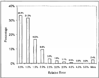
Figure 2 shows the distribution of relative error among all tested cases with the summary data in T a b l e 1. The percentage of estimates whose relative error was greater than 5% is 2.4%, less than 5%. We also can see that the percentage of estimates whose relative error is greater than 2.5% is not too big, only 5.9%. These results show that the estimates are still a little conser­ vative.

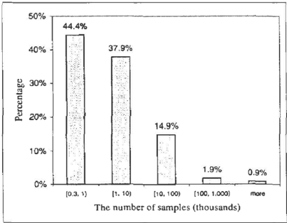
Figure 3 shows the distribution of the minimum re­ quired number of samples to satisfy the precision re­ quirement (a 2.5% relative error with 2.5% failure probability). We can see that only 2.8% data ex­ ceeded our upper limit of 100,000 on the number of

Table 1:Summary relative error for the CPCS network. See Figure 2.

		Min	Median	Max
1.1%	1.6%	0.00049%	0.75%	18.8%

samples. More than 80% of the estimates required less than 10,000 samples and almost half required less than 1,000 samples. Based on a Pentium II, 450 MHz Win­ dows computer, the correspondence between the num­ ber of samples and the execution time in the CPCS network with 20 evidence nodes in our experiments is as follows. Learning the importance function took about 6.3 seconds. Without learning, the algorithm generated about 5,880 samples per second. So, 10,000

samples needed only about 1. 7 seconds. About half of the estimates needed only 1,000 samples. As we suggested before, if after several updating stages, we find that the minimum number of samples needed to reach the required precision is still prohibitive, it may pay to restart the process with a different initializa­ tion method. In our experiment, we have tried another method. If the required number of samples was pro­ hibitive (greater than our upper limit of 100,000 sam­ ples), we called the function Estimate.Prob(W = w ) again. About 60% of such cases were eliminated in the second call, i.e., a different random number seed partially solved the problem.

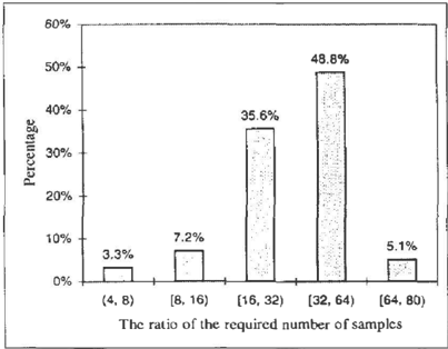
We also compared the efficiency of the AIS-BN-a al­ gorithm with the efficiency of the AIS-BN-p algo­ rithm. Using inequality (3) a n d the estimated values band jl, we can calculate a N for the AIS-BN-p algo­ rithm. Figure 4 shows the ratio between this number and the number obtained from the AIS-BN-a algo­ rithm. We can see that AIS-BN-t-t required at least four times the number of samples required by AIS­ BN-a. The maximum times were as high as 79.4 sec­ onds. 89.5% of the test cases required over 16 times number of samples. From these data we conclude that the AIS-BN-a algorithm is significantly better than the AIS-BN-t-t algorithm. Even if the value of a is es­ timated conservatively, it can still lead to large savings in computation.

7 Conclusion

We presented two algorithmsAIS-BN-t-t and AIS­ BN-a for confidence probabilistic inference in Baye­ sian networks. These algorithms can guarantee that

the estimated results are the (er, J) relative approxi­ mation of the exact values if we know the exact values of the upper bound b and the variance 0" 2 of the esti­ mated random variable. If we do not know these val­ ues, we can use the estimated b and 0"2 to estimate the minimum required number of samples N. Although this estimation method introduces error, our exper­ imental results show that the approximation is still reasonable and conservative. By learning the optimal importance function, sampling algorithms with the es­ timation algorithms can provide substantial computa­ tional savings. While they are heuristic in nature, they perform excellent in practice.

Our experiments have also shown that the AIS-BN0" algorithm seems to be significantly better than the AIS-BN-J.L algorithm and our recommendation is to adopt it in practical belief updating algorithms. Al­ though in this paper we base the AIS-BN-,u and AIS­ BN-O" algorithms on the AIS-BN algorithm, our re­ sults are applicable to other sampling algorithms, as long as these algorithms generate independent sam­ ples.

Acknowledgements

This research was supported by the National Science Foundation under Faculty Early Career Development (CAREER) Program, grant IRI�9624629, and by the Air Force Office of Scientific Research under grant number F49620�00�1�0112. Malcolm Pradhan and Max Henrion of the Institute for Decision Systems Research shared with us the CPCS network with a kind permission from the developers of the Internist system at the University of Pittsburgh. Jeff Schnei­ der and anonymous reviewers provided us with use­ ful suggestions for improving the clarify of the pa­ per. All experimental data have been obtained us­ ing SMILE, a Bayesian inference engine developed at the Decision Systems Laboratory and available at http://www2.sis.pitt.edu/�genie.

References

[Chavez and Cooper, 1990] Martin R. Chavez and Gregory F. Cooper. A randomized approximation algorithm for probabilistic inference on Bayesian belief networks. Networks, 20(5):661-685, August 1990.

[Cheng and Druzdzel, 2000) Jian Cheng and Marek J. Druzdzel. AIS-BN: An adaptive importance sam­ pling algorithm for evidential reasoning in large Ba­ yesian networks. Journal of Artificial Intelligence Research, 13:155�188, 2000.

• [Cheng, 2001] Jian Cheng. Sampling algorithms for estimating the mean of bounded random variables. Computational Statistics, 16(1):1-23, 2001.
• [Dagum and Horvitz, 1993] Paul Dagum and Eric Horvitz. A Bayesian analysis of simulation algo­ rithms for inference in belief networks. Networks, 23:499�516, 1993.

[Dagum and Luby, 1997] Paul Dagum and Michael Luby. An optimal approximation algorithm for Ba­ yesian inference. Artificial Intelligence, 93:1�27, 1997.

[ Dagum et al., 2000] Paul Dagum, Richard Karp, Michael Luby, and Sheldon Ross. An optimal al­ gorithm for Monte Carlo estimation. SIAM Journal on computing, 29(5):1481�1496, 2000.

[Fishman, 1995] George S. Fishman. Monte Carlo: concepts, algorithms, and applications. Springer­ Verlag, 1995.

[Fung and Chang, 1989] Robert Fung and Kuo-Chu Chang. Weighing and integrating evidence for stochastic simulation in Bayesian networks. In Un­ certainty in Artificial Intelligence 5, pages 209�219, New York, N. Y., 1989. Elsevier Science Publishing Company, Inc.

[Pearl, 1988] Judea Pearl. Probabilistic Reasoning in Intelligent Systems: Networks of Plausible Infer­ ence. Morgan Kaufmann Publishers, Inc., San Ma­ teo, CA, 1988.

[ Pradhan and Dagum, 1996] Malcolm Pradhan and Paul Dagum. Optimal Monte Carlo inference. In Proceedings of the Twelfth Annual Conference on Uncertainty in Artificial Intelligence (UAI-96), pages 446�453, San Francisco, CA, 1996. Morgan Kaufmann Publishers.

[Pradhan et al., 1994] Malcolm Pradhan, Gregory Provan, Blackford Middleton, and Max Henrion. Knowledge engineering for large belief networks. In Proceedings of the Tenth Annual Conference on Un­ certainty in Artificial Intelligence (UAI-94), pages 484�490, San Mateo, CA, 1994. Morgan Kaufmann Publishers, Inc.

[Shachter and Peat, 1989] Ross D. Shachter and Mark A. Peat. Simulation approaches to general probabilistic inference on belief networks. In Un­ certainty in Artificial Intelligence 5, pages 221�231, New York, N. Y., 1989. Elsevier Science Publishing Company, Inc.

[ Shimony, 1994] Solomon E. Shimony. Finding MAPs for belief networks is NP-hard. Artificial Intelli­ gence, 68(2):399-410, August 1994.