Empirical Evaluation of Approximation Algorithms for Probabilistic Decoding

Irina Rish, Kalev Kask and Rina Dechter*

Department of Information and Computer Science University of California, Irvine { irinar, kkask, dechter} @ics. uci. edu

Abstract

It was recently shown that the problem of de­ coding messages transmitted through a noisy channel can be formulated as a belief up­ dating task over a probabilistic network (14). Moreover, it was observed that iterative ap­ plication of the ( linear time ) belief propa­ gation algorithm designed for polytrees (15) outperformed state of the art decoding algo­ rithms, even though the corresponding net­ works may have many cycles.

This paper demonstrates empirically that an approximation algorithm approx-mpe for solving the most probable explana­ tion ( MPE ) problem, developed within the recently proposed mini-bucket elimination framework (4), outperforms iterative belief propagation on classes of coding networks that have bounded induced width. Our ex­ periments suggest that approximate MPE de­ coders can be good competitors to the ap­ proximate belief updating decoders.

1 Introduction

In this paper we evaluate the quality of a recently proposed mini-bucket approximation scheme (8, 6) for probabilistic decoding.

Recently, a class of parameterized mini-bucket approx­ imation algorithms for probabilistic networks, based on the bucket elimination framework, was proposed in (4). The approximation scheme uses as a control­ ling parameter a bound on arity of probabilistic func­ tions ( i.e., clique size ) created during variable elimi­ nation, allowing a trade-off between accuracy and effi­ ciency (8, 6). The mini-bucket algorithms were pre­ sented and analyzed for several tasks, such as be­ lief updating, finding the most probable explanation

*This work was partially supported by NSF grant IRI9157636 and by Air Force Office of Scientific Research grant, AFOSR 900136, Rockwell International and Amada

of America.

( MPE ) and finding the maximum a posteriori hypoth­ esis ( MAP ) . Encouraging results were obtained on ran­ domly generated noisy-OR networks and on the CPCS networks (16). Clearly, more testing is necessary to de­ termine the regions of applicability of this class of algo­ rithms. In particular, testing on realistic applications is mandatory.

When it was recently shown that the problem of decod­ ing noisy messages can be described as a belief updat­ ing task over a probabilistic network (14], we decided to use this problem as our next benchmark. This domain was particularly interesting since the recent advances in probabilistic decoding demonstrated that the ( lin­ ear time ) belief propagation algorithm for polytrees (15) yields a nearly optimal decoder if applied iteratively to multiply-connected coding networks, such as low­ density parity-check codes (13], low-density generator matrix codes (3), and, especially, turbo codes [ 2 ] . This is considered "the most exciting and potentially im­ portant development in coding theory in many years" (14). Initial analysis of iterative belief propagation on networks with loops is presented in [ 2 0] .

In this paper we compare the mini-bucket MPE ap­ proximation algorithm approx-mpe to the iterative be­ lief propagation (IBP), and to the exact elimination algorithms elim-mpe, elim-map and elim-bel for MPE, MAP and for belief updating, respectively, on several classes of linear block codes, such as Hamming codes, randomly generated block codes, and structured low­ induced-width block codes. A codeword is transmit­ ted through a channel adding a Gaussian noise to each bit. Given the real-valued channel output y, the task of decoding is to find the most likely assignment ei­ ther to each information bit ( bit-wise decoding ) , or to the whole information sequence ( block-wise decod­ ing ) (14, 10, 11]. Other variation ( not considered here ) could be to round y to a 0/1 vector before decoding.

This paper demonstrates empirically that

1. on a class of structured codes having low induced width the mini-bucket approximation approx-mpe out­ performs IBP;

2. on a class of random networks having large induced width and on some Hamming codes IBP outperforms

approx-mpe;

1. as expected, exact MPE decoding, elim-mpe, out­ performs approximate decoding. However, on random networks exact MPE decoding was not feasible due to the large induced width (as it is known, variable elimi­ nation algorithms are exponential in the induced width of the network).
2. The exact MPE (maximum-likelihood) ( elim-mpe) and the exact belief update decoding ( elim-beQ have comparable error for relative low channel noise; for larger noise, belief update decoding gives a slightly smaller (by� 0.1%) bit error than the MPE decoding.

2 Definitions and notation

Definition 1: [graph concepts) A directed graph is a pair G = {V, E}, where V = {X 1 , . . . , X n} is a set of nodes, or variables, and E = {(X;, Xj) IX;, Xj E V} is the set of edges. Given (X;, Xj) E E, X; is called a parent of Xj, and Xj is called a child of X;. The set of X;'s parents is denoted pa(X;), or pa;, while the set of X;'s children is denoted ch (X;), or ch;. The family of X; includes X; and its parents. A directed graph is acyclic if it has no directed cycles. A graph is singly connected (also called a polytree), if its under­ lying undirected graph has no cycles. Otherwise, it is called multiply connected. An ordered graph is a pair ( G, o ) where o = X 1, ... , Xn is an ordering of the nodes in the graph G. The width of a node in an ordered graph is the number of the node's neighbors that pre­ cede it in the ordering. The width of an ordering o, denoted w ( o ) , is the maximum width over all nodes. The induced graph of G along an ordering o is obtained by connecting the preceding neighbors of each x;, go­ ing from XN to x1. The induced width of a graph along an ordering o, w ; , is the width of the induced graph along o. The induced width of a graph, W*, is the min­ imal induced width over all its orderings; w * + 1 is also called tree-width [1]. For more information see [9, 7]. The moral graph of a directed graph G is the undi­ rected graph obtained by connecting the parents of all the nodes in G and removing the arrows.

Definition 2: [belief networks] Let X = {X1, ... , X n } be a set of random variables over multivalued do­ mains D1, ... , Dn. A belief network (BN) is a pair (G, P) where G is a directed acyclic graph on X and P = {P(X;Ipa;)li = 1, ... , n} is the set of conditional probability matrices associated with each X;. An as­ signment (X1 = x1, ... ,Xn = Xn) can be abbreviated as x = (x1, ... , Xn)· The BN represents a joint proba­ bility distribution P( X1, .... , Xn) = IIi'=l P( Xi lx p a ( x , ) ), where xs is the projection of vector x on a subset of variables S. An evidence e is an instantiated subset of variables.

Given evidence e, the following tasks can be defined over a belief network. 1. Belief updating: find­ ing the posterior probability P(Yie) of a query nodes Y E X; 2. Most probable explanation (MPE): finding an assignment X0 = ( x 0 1 , ··. ,X0n), such that p( x0 ) = maxx P( x i e ). 3. Maximum aposteriory hypothesis (MAP): finding an assignment a0 = (a01, . . . , a0k) to a subset of variables A= {A1, ... ,Ak}, called a hypoth­ esis, such that p(a0) = ma:xak LP( x i e ), where �x-A ak = {A1 = a1, . . . , Ak = ak}.

3 Noisy channel coding

The purpose of channel coding is to provide reliable communication through a noisy channel. A system­ atic error-correcting encoding [14] maps a vector of K information bits u = (u1, ... , uK), u; E {0, 1}, into an N-bit codeword c = (u, x), where NI< additional bits x = (x1, ... , XN-K), X j E { 0 , 1} add redundancy to the information source in order to decrease the de­ coding error. The codeword, called the channel input, is transmitted through a noisy channel. A commonly used Additive White Gaussian Noise (A WGN) channel model implies that independent Gaussian noise with variance u2 is added to each transmitted bit, produc­ ing the channel output y. Given a real-valued vector y, the decoding task is to restore the input information vector u [10, 14, 13]. An alternative approach, not considered here, is to round y to a 0/1 vector before decoding.

The probability of decoding error is measured by the bit error rate (BER}, i.e. the percentage of incorrectly decoded bits. The code rate R = J{ / N is the fraction of the information bits to the total number of transmit­ ted bits. The goal is to minimize the decoding error while maintaining a relatively low code rate. Shan­ non [19] proved that there exists a lower bound, called Shannon's limit, to the decoder's performance. Given the noise variance u2 and a fixed code rate R, Shan­ non's limit gives the smallest achievable BER no mat­ ter which code is used. Unfortunately, Shannon's proof was nonconstructive, leaving open the problem of find­ ing optimal codes. Moreover, it assumes an optimal maximum-likelihood decoding, which is intractable for high-performance codes that tend to be long [17]. "As far as is known, a code with a low-complexity optimal decoding algorithm cannot achieve high performance" [14]. Therefore, good codes should be combined with efficient approximate decoding algorithms into high­ performance coding schemes.

Recently, several low-error coding schemes have been proposed, such as turbo-codes [2], low-density parity­ check c�des [13] and low-density generator matrix codes [3], that achieve a near-Shannon-limit perfor­ mance. It was shown, that the decoding algorithms used by turbo-codes and some other low-error codes can be viewed as an iterative application of the belief propagation algorithm [15], designed for polytrees, to multiply-connected coding networks.

In this paper, we report on experiments with several types of linear (N,K} block codes. A linear (N ,K) block code can be defined in terms of a generator matrix

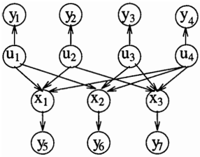
or in terms of a parity check matrix (1 4 ] . Given a 0/1 generator matrix G, and an information vector u, the codeword c = (u, x) must satisfy c = u G , where summation modulo 2 is assumed. For example, the generator matrix

defines a (7,4) Hamming code. It can be depicted by the belief network in Figure 1, that represents each bit in u, x, and y vectors as a node. The parent set for each Xi corresponds to non-zero entries in (K + i ) th column of G, and the deterministic conditional proba­ bility function P ( x i i Pa i ) equals 1 iff Xi= uit Ef) ... Ef)ujp, where Ef) is addition modulo 2. The bits Xi are also called the parity-check bits. Note, that this structure is a special ( deterministic ) case of causal independence, which can be exploited to speed up probabilistic infer­ ence (12, 21, 1 8 ] . Each output bit Yi has exactly one parent, the corresponding channel input bit. The con­ ditional density function P ( y j lei) is a Gaussian ( nor­ mal ) distribution N(cj; 0' ) , where the mean equals the value of the transmitted bit, and 0' 2 is the noise vari­ ance.

Probabilistic decoding can be formulated either as maximum aposteriory information bit decoding, or as a maximum aposteriory ( maximum-likelihood ) infor­ mation sequence (block) decoding. Formally, given the observed output y, the first task is to find for each k

while the second is to find

An alternative formulation of block-wise decoding is to find a most probable explanation ( MPE ) assignment to all codeword bits

Therefore, the bit-wise decoding requires finding pos­ terior probabilities for each information bit and can be

Algorithm elim-mpe

Input: A belief network BN = {Pt, ... , Pn}; a variable ordering o;

Output: The most probable assignment X*.

an evidence e = {(X; = v; )l X; E Y, Y C X}.

1. Initialize: Partition BN into bucket1, . . . , bucketn, s.t. bucket; contains all Pj whose highest variable is X;. Put each observation (X; = v; ) into bucket;.
2. Let h1, h2, ... , hj be the functions in bucketp, and let S1, ... , Sj be the subsets of variables on which hj are de­ fined.
3. Backward: For p <-- n downto 1, do
4. If bucketp contains Xp = vp, I* evidence *I assign Vp to Xp in each h; and put the result into an appropriate bucket.
5. Else, compute hP: hP = maxxPII{=1h;. Add hP to the bucket of the largest-index variable in Up <-ULl S; - {Xp}.
6. Forward: Assign optimal values to Xp along the ordering 0, as follows: x; = arg maXXp hP.

Figure 2: Algorithm elim-mpe

solved by belief updating algorithms, while the block­ wise decoding requires algorithms for finding MAP or MPE. In the next section, we discuss exact and ap­ proximate algorithms for these tasks.

4 Algorithms

In this section we present the algorithms to be eval­ uated on coding problems. We start with a brief de­ scription of the bucket-elimination framework, that in­ cludes the algorithms elim-bel, elim-mpe, and elim­ map for computing exact belief, MPE, and MAP, respectively ( 4 ] , and the mini-bucket approximation approx-mpe(i) for MPE (8, 6]. Then we present the Iterative Belief Propagation (IBP) algorithm.

4.1 Bucket-elimination algorithms

Bucket elimination was introduced recently as a uni­ fying variable elimination algorithmic framework for probabilistic and deterministic reasoning (5]. In partic­ ular, it was shown that many algorithms for probabilis­ tic inference, such as belief updating, finding the most probable explanation, finding the maximum aposteri­ ori hypothesis, and calculating the maximum expected utility, can be expressed as bucket-elimination algo­ rithms ( 4 ] .

The input to a bucket-elimination algorithm consists of a knowledge-base theory specified by a collection of functions or relations, ( e.g., clauses for proposi­ tional satisfiability, constraints, or conditional prob­ ability matrices for belief networks ) . Given a variable ordering, the algorithm partitions the functions into buckets, each associated with a single variable, and process the buckets in reverse order, from last vari­ able to first. Each bucket is processed by some vari-

Algorithm approx-mpe(i)

Input: A belief network BN = {Pt, ... , P n } ; a variable ordering o; an evidence e = {(X; = v; )l X; E Y, YcX}.

Output: An upper and lower bounds on the most prob­ able assignment.

1. Initialize: Partition BN into bucket1, . . . , bucketn, s.t. bucket; contains all Pj whose highest variable is X;. Put each observation (X; = v; ) into bucket;.
2. Let h 1 , h2, ... , hj be the functions in bucketp, and let 81, ··· , Sj be the subsets of variables on which hj are de­ fined.
3. Backward: For p <- n downto 1, do
4. (evidence) If bucketp contains Xp = v p , assign Vp to Xp in each h; and put the result into an appropriate bucket.
5. else, //for ht, h2, ... , hj in bucketp,

Generate an i-partitioning, Q = { Q1, ... , Qr }, tions ht, h2, ... , hi in bucketp.

• do: ' of func­

For each Q, E Q ' containing h 1 1, ··· h 1 1 do,

Generate function h 1 , h 1 = maxxPII�=Ihl;· Add h 1 to the bucket of the largest-index variable in U 1 <-U:=I s, , -{ Xp } ·

3. Forward: For p = 1 to n do: given x1, ... ,Xp-1, assign to Xp a value Vp that maximizes the product of all the functions in bucketp.

Figure 3: algorithm approx-mpe(i)

able elimination procedure over the functions in the bucket, and the resulting new function is placed in a lower bucket.

Figure 2 shows elim-mpe, the bucket-elimination algo­ rithm for computing MPE [4]. Given a variable or­ dering, the conditional probability matrices are parti­ tioned into buckets, where each matrix is placed in the bucket of the highest variable it mentions. When pro­ cessing the bucket of Xp, a new function is generated by taking the maximum relative to Xp, over the prod­ uct of functions in that bucket. The resulting function is placed in the appropriate lower bucket. The algo­ rithms elim-bel and elim-map for belief updating and for finding MAP are derived in a similar way [4].

The complexity of the bucket elimination algorithms is determined by the complexity of processing each bucket ( step 2), and is time and space exponential in the number of variables in the bucket. This number equals w * + 1, where w * is the induced-width of the of the network's moral graph along the given variable ordering.

4.2 Mini-bucket algorithms

Since elimination becomes intractable when the func­ tions hp created in the buckets are too large, we pro­ posed in [8] to approximate these functions by a collection of smaller functions. Let h1, ... , hj be the functions in the bucket of Xp, and let S1, ... , Sj be the variable subsets on which those functions are defined. When elim-mpe processes the bucket of Xp, it computes the function hP: hP = maxxpii { =1hi. A brute-force ap­ proximation method involves migrating the maximiza­ tion operator inside the multiplication, generating in­ stead a new function gP: gP = rr { =lmaxxphi. Obvi­ ously, hP ::; gP. Each maximized function will have the arity lower than the arity of hi, and each of these functions can be moved, separately, to a lower bucket. When the algorithm reaches the first variable, it has computed an upper bound on the MPE. A maximizing tuple can then be generated by instantiating the vari­ ables going from first bucket to last, using the informa­ tion that is recorded in each bucket. The probability of the tuple is the lower bound on the MPE.

This idea was extended to yield a collection of pa­ rameterized approximation algorithms by partitioning the bucket into mini-buckets of varying sizes and ap­ plying the elimination operator on each mini-bucket rather then on single function. This yields approxima­ tions of varying degrees of accuracy and efficiency. Let Ql = { Q1, .. . , Qr} be a partitioning into mini- buck­ ets of the functions h1, ... , hj in Xp 's bucket. If the mini-bucket Q1 contains the functions h1u ... , h1r, the approximation will compute g P = IT/=1maxx P III,hl,· Clearly, coarser partitionings yield the higher accu­ racy, but also the higher complexity.

Algorithm approx-mpe(i) is described in Figure 3. It is parameterized by the bound i on the number of vari­ ables allowed in a mini-bucket. A partitioning Q into mini-buckets is an i-partitioning if the total number of variables in each mini-bucket does not exceed i.

It was shown [8] that algorithm approx-mpe ( i ) com­ putes an upper bound to the MPE in time and space 0( exp( i )) where i ::; n.

4.3 Iterative belief propagation

Iterative Belief Propagation ( IBP ) computes an ap­ proximate belief for every variable in the network. It applies Pearl's belief propagation algorithm [15], de­ veloped for singly-connected networks, to a multiply­ connected networks, ignoring cycles. Belief is prop­ agated by sending messages between the nodes: for each node x, its parents Ui send causal support mes­ sages '1ru;,x1 while its children Yi send diagnostic sup­ port messages Ay;,x· Causal supports from all parents and diagnostic support from all children are combined into vectors 'lrx and Ax, respectively.

An activation schedule ( variable ordering ) A specifies the order in which the nodes are processed ( activated ) . After all nodes are processed, the next iteration of be­ lief propagation begins, updating the messages com­ puted during the previous iteration. Algorithm IBP ( n ) stops after n iterations. Note, that the algorithm is not guaranteed to converge to the correct beliefs on multiply-connected networks.

The algorithm is given in figure 4. It takes a variable ordering as an input. We have used an ordering that

Iterative Belief Propagation (IBP)

Input: A Belief Network BN = {P1, ... ,Pn}, evidence e, an activation schedule A, the number of iterations I. Output: Belief in every variable.

1. Initialize A and 11".

For evidence node x; = j, set A..,,(k) to 1 for j = k and to 0 for j of. k. For node x having no parents set 11"x to prior P(x ) . Otherwise, set Ax and 11"x to (1, . . . , 1 ) .

1. For iterations = 1 to /: For each node x along A, do:

f* a is a normalization constant * /

• For each x = j, compute Ax,u; (j) =
• Q' L:j Ax(j) l:: ul :! ;l i P(x = j I Ul, .·· ,urn ) nl;li 11"ul·"'
• For each x = j, compute 11"x, y ; (j) =
• Q' nk;li Ay k, x(j) 2:: .. 1 P(x = j I Ul, ... , Um ) TI!11"ul·"'"
• Belief update: For each x along A
• For each x = j, compute
• Ax(j) = fl; Ay;,x(j), where y; are x's children.
• For each x = k, compute
• 1r..,(j) = "\"' P(x = j I u1, ... ,urn ) fi-11"u;,x, L...t u 1 , ... ,um ' where u; are x's parents.
• Compute BEL(x) = ll'Ax11"x·

Figure 4: Iterative Belief Propagation (IBP) Algo­ rithm

first updates the input variables of the coding network and then updates the parity-check variables. Notice that evidence variables are not updated.

5 Experimental Methodology

We experimented with several types of (N, K) linear block codes, which include (7, 4) and (15, 11) Ham­ ming codes, randomly generated codes, and structured codes with low induced width. So far, we used only the code rate R= 1/2, i.e. N = 2K.

Both random and structured code networks have a fixed number of parents, P. In random codes, for each parity-check bit Xj, P parents are selected ran­ domly out of K information bits. In structured parity­ check codes, each parity bit Xi has P sequential parents {u ( i +j)modK , O 5 j < P}.

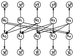
Our random and structured codes can be represented as four-layer belief networks having K nodes in each layer (see Figure 5). The two inner layers (channel input nodes) correspond to the input information bits Ui, 0 :::; i < K, and to the parity-check bits, Xi, 0 5 i < K. The two outer layers represent the channel output y = (y«, yx), where y« and yx result from transmitting u and x, respectively. The input nodes are binary (0/1), while the output nodes are real-valued.

Given K, P, and the channel noise variance u 2 , a sam­ ple coding network is generated as follows. First, the appropriate belief network structure is created. Then,

we simulate an input signal assuming uniform random distribution of information bits, and the corresponding values of the parity-check bits are computed. Finally, we generate an assignment to the observed vector y by adding Gaussian noise to each information and parity­ check bit. The decoding algorithm takes as an input the coding network and the observed channel output y (a real-valued assignment to the yf and Yi nodes). Tpe task is to recover the original information sequence.

We experimented with the following decoding algo­ rithms: iterative belief propagation (IBP), the exact elimination algorithms for belief updating and finding MAP and MPE (elim-bel, elim-map and elim-mpe, respectively), and approx-mpe(i) algorithm. When i < P, the number of variables in a mini-bucket is bounded by max(i, P + 1), rather than by i. IBP(I) denotes iterative belief propagation with I iterations.

For each decoding algorithm, we plot the observed bit error rate (BER) versus the channel parameter u.

In all our experiments the BER of elim-map coincided with that of elim-mpe, and will not be reported sepa­ rately.

6 Results and Discussion

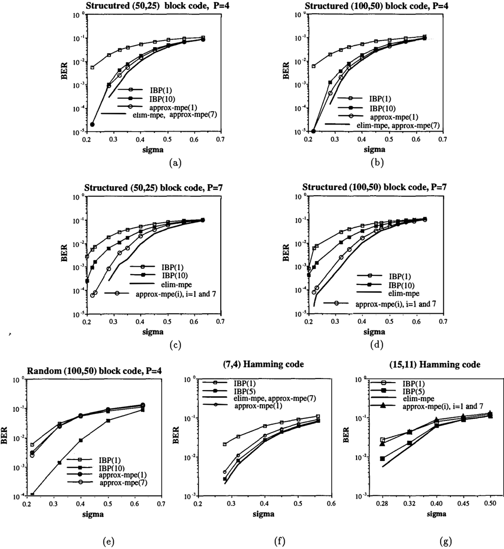
The results on the three classes of coding networks are summarized in Figures 6(a)-(g). For more details, see table 2.0n the class of parity-check codes we ran up to 10 iterations of IBP and report the results for IBP(1) and IBP(10).

Algorithm approx-mpe(i) was tested for several values of i. Its accuracy increases with increasing i, and the algorithm becomes exact for i > w * , where w * is the induced width of the network.

6.1 Exact MPE versus exact belief-update decoding

Before testing the approximation algorithms for bit­ wise and block-wise decoding, we tested whether there is a significant difference between the corresponding exact decoding algorithms. We compared exact elim­ mpe against exact elim-bel on several types of net-

works, including two Hamming code networks, ran­ domly generated networks with different number of parents, and structured code. The results for 1000 in­ put signals, generated randomly for each network, are presented in Table 6.1. When noise is relatively low ( IT = 0.3), both algorithms have practically the same decoding error, while for larger noise (IT = 0.5) the bit­ wise decoding (elim-bel) gives a slightly smaller BER than the block-wise decoding (elim-mpe).

6.2 Structured parity-check codes

Comparison of the algorithms on the structured parity-check code networks with K=25 and 50, and P=4 and 7 (figure 6( a)-( d)) shows that:

1. as expected, exact elim-mpe decoder always gives the smallest error;
2. IBP(10) is more accurate on average than IBP(1); however, this may not be the case on some particular instances;
3. as expected, approximation algorithm elim-mpe(i) is close to elim-mpe, due to the low induced width of the networks ( w* = 6 for P=4, and w* = 12 for P=7).
4. algorithm elim-mpe(i) outperforms IBP and IBR on all structured networks.

With increasing the parents set size from P =4 (fig­ ures 6(a) and 6(b)) to P =7 (figures 6(c) and 6(d)), the difference between IBP and elim-mpe(i) becomes even more pronounced. On networks with P=7 both approx-mpe(1) and approx-mpe(7) achieve an order of magnitude smaller error than IBP(10).

Next, we consider the results for each algorithm sep­ arately, increasing the number of parents from P =4 to P =7 (see also Table 2). We see that the error of IBP(1) practically does not change, the error of the exact elim-mpe changes only slightly, while the error ofiBP(10) and approx-mpe(i) increases. However, the BER of IBP(10) increased more dramatically with in­ creased parent set. The induced width of the network was increasing with the increasing parent set size, and affected the quality of both IBP and approx-mpe(i). In case of P=4 (induced width 6), approx-mpe(7) coin­ cides with elim-mpe; in case of P=7 (induced width 12) approximation algorithms do not coincide with elim­ mpe. Still, they are better than IBP.

In summary, the results on structured parity-check codes demonstrate that approx-mpe(i), even for i=1, was always at least as accurate as belief propagation with 10 iterations. On networks with larger parent sets approx-mpe(1) and approx-mpe(7) were an order of magnitude better than IBP(10), and about two or­ ders of magnitude better than IBP(1). These results indicate that approx-mpe(i) may be a better decoder than IBP on the networks having relatively small in­ duced width.

6.3 Random parity-check code

On randomly generated parity-check networks (Fig­ ure 6( e)) the picture was reversed: approx-mpe(i) was worse than IBP(10), although as good as IBP(1). Elim-mpe always ran out of memory on those net­ works (the induced width exceeded 30). The results are not surprising since approx-mpe(i) is not likely to be accurate if the bound i is much lower than the in­ duced width. However, it is not clear why IBP was much better in this case. We also need to compare our algorithms on other random code generators such as recently introduced in coding community low-density generator matrix [3] and low-density parity-check[13] code.

6.4 Hamming codes

We tested the belief propagation and the mini-bucket approximation algorithms on two Hamming code net­ works, one with K = 4, N = 7, and the other one with K = 11, N = 15. The results are shown in fig­ ures 6(f) and 6(g). Again, the most accurate results are produced by elim-mpe decoding. Since the induced width of the (7,4) Hamming network is only 3, approx­ mpe(7) coincides with the exact algorithm. IBP(1) is much worse than the rest of the algorithms, while IBP(5) is very close to the exact elim-mpe. Algorithm approx-mpe(1) is slightly worse than IBP(5). On the larger Hamming code network, the results are similar, except that both approx-mpe(1) and approx-mpe(7) are inferior to IBP(5), which is inferior to elim-mpe. These results are expected since the induced width of the network is larger ( w* = 9), so that approximation with bound 7 or less is suboptimal. Since the networks were quite small, the runtime of all algorithms was less than a second, and the time ofiBP(5) was comparable to the time of exact elim-mpe.

In summary, we see that MPE decoding is always supe­ rior to IBP decoding. It is expected that an optimal algorithm will be superior, however, since elim-mpe minimizes the block error, while IBP minimizes the bit error, this was not completely clear. For structured parity-check networks having bounded induced width, approx-mpe(i) also outperforms IBP by order(s) of magnitude. However, when the induced width is large (e.g., random parity-check codes), approx-mpe(i) is less accurate than IBP.

7 Conclusions

This paper studies empirically the performance of sev­ eral approximate probabilistic inference algorithms on the probabilistic decoding problem. The mini-bucket approximation algorithms for finding a most probable explanation (MPE) are compared against the follow­ ing algorithms: exact elim-mpe, elim-map, elim-bel, and a variation of Pearl's belief propagation algorithm. The latter was shown recently to be a highly effective

Table 1: BER of exact decoding algorithms elim-bel ( denoted bel) and elim-mpe ( denoted mpe) on several block codes ( average on 1000 randomly generated input signals ) .

CT	Hamming code				Random code						Structured code
	7,4 .I		15,11		K 10, N 20, p I 3		K 10, N 20, p, 5		K 10, N 20, p 7		K 25, P-4
	,. ._	mpe	_,.	mpe	_,_.	mpe	,_.	mpe	De	mpe	be	mpe
0.3	6.7e-3	6.8e-3	1.6e-2	1.6e-2	1.8e-3	1.7e-3	5.0e-4	5.0e-4	2.1•-3	2.1e-3	6.4e-4	6.4e-4
0.5	9.8e-2	l.Oe-1	l.Se-1	1.6e-1	8.2e-2	8.5e-2	8.0e-2	8.1e-2	8.7e-2	9.1e-2	3.9e-2	4.1e-2

decoder if applied iteratively to coding networks. We evaluated these algorithms on linear block codes of sev­ eral types: Hamming codes, structured codes with low induced width, and randomly generated codes.

Our results show that in coding networks inducing small width, the mini-bucket algorithms outperformed the iterative belief propagation. However, for networks having a large induced-width ( e.g., random codes ) and for Hamming codes the iterative approach outper­ formed the basic mini-bucket algorithm. In all cases, and as is quite expected, decoding using the optimal elim-mpe algorithm was best.

As expected, we observe dependence between the net­ work's induced-width and the quality of the mini­ bucket's approach; such dependence is less clear for iterative belief propagation. We also observe increased accuracy as we employ more powerful mini-bucket al­ gorithms.

Our experiments were restricted to networks having small parent sets since the mini-bucket approach and the belief propagation approaches are, in general, time and space exponential in the parent set. This limita­ tion can be eliminated in using the specific structure of coding networks that is a particular ( deterministic ) case of causal independence [12, 21). Such networks can be transformed into networks having families of size three only. Indeed, in coding practice, the be­ lief propagation algorithm is linear in the family size, thus allowing processing networks of arbitrary family size. We plan to exploit causal independence in the mini-bucket algorithms as well, and hope to extend our experimental evaluation accordingly.

Acknowledgments

We wish to thank Padhraic Smyth and Robert McEliece for insightful discussions and providing var­ ious information about the coding domain.

References

1. S. Arnborg, D.G. Corneil, and A. Proskurowski. Complexity of finding embedding in a k-tree. Journal of SIAM, Algebraic Discrete Methods, 8(2):177-184, 1987.
2. G. Berrou, A. Glavieux, and P. Thitimajshima. Near shannon limit error-correcting coding: turbo

I

I

I

I

• codes. In Proc. 1993 International Conf. Comm. (Geneva, May 1993}, pages 1064-1070, 1993.
• J.-F. Cheng. Iterative decoding. PhD Thesis, 1997.
• [4) R. Dechter. Bucket elimination: A unifying framework for probabilistic inference. In Proc. Twelfth Conf. on Uncertainty in Artificial Intel­ ligence, pages 211-219, 1996.
• R. Dechter. Bucket elimination: a unifying frame­ work for processing hard and soft constraints. CONSTRAINTS: An International Journal, 2:51 - 55, 1997.
• R. Dechter. Mini-buckets: A general scheme for generating approximations in automated rea­ soning. In Proc. Fifteenth International Joint Conference of Artificial Intelligence (IJCAI-97}, Japan, pages 1297-1302, 1997.
• [7) R. Dechter. Bucket elimination: A unifying framework for probabilistic reasoning. In M. I. Jordan ( Ed. ) , Learning in Graphical Models, Kluwer Academic Press, 1998.
• [8) R. Dechter and I. Rish. A scheme for approx­ imating probabilistic inference. In Proc. Thir­ teenth Conf. on Uncertainty in Artificial Intelli­ gence, 1997.
• [9) Rina Dechter and Judea Pearl. Network-based heuristics for constraint-satisfaction problems. Artificial Intelligence, 34:1-38, 1987.
• B.J. Frey. Bayesian networks for pattern classi­ fication, data compression, and channel coding. PhD Thesis, 1997.
• B.J. Frey and D.J.C. MacKay. A revolution: Be­ lief propagation in graphs with cycles. Advances in Neural Information Processing Systems, 10, 1998.
• D. Heckerman and J. Breese. A new look at causal independence. In Proc. Tenth Conf. on Uncer­ tainty in Artificial Intelligence, pages 286-292, 1994.
• D.J.C. MacKay and R.M. Neal. Near shannon limit performance of low density parity check codes. Electronic Letters, 33:457-458, 1996.
• R.J. McEliece, D.J.C. MacKay, and J.-F.Cheng. Turbo decoding as an instance of pearl's belief propagation algorithm. To appear in IEEE J. Se­ lected Areas in Communication, 1997.

Table 2: Bit error rate and runtime of the algorithms on structured a block codes. Notation: ( 1 ) is IBP ( 1 ) , ( 2 ) is IBP ( 10 ) , ( 3 ) is elim-mpe, (4) is approx-mpe ( 1 ) , ( 5 ) is approx-mpe ( 7 ) .

u	BER					Time
	1	2	3	4	5	I 1	2	3	4	5
K:_25, P-4, R-lf2, 1000 experiments per row
induced width = 6
0.28	1.8e-2	l.Oe-3	2.8e-4	8.8e-4	2.8e-4	0.02	0.16	0.03	0.01	0.04
0.32	3.0e-2	4.1e-3	1.1e-3	2.5e-3	1.1e-3	0.02	0.16	0.03	0.02	0.04
0.35	3.8e-2	7.4e-3	3.2e-3	5.4e-3	3.2e-3	0.02	0.16	0.03	0.02	0.04
0.40	5.2e-2	1.7e-2	l.Oe-2	1.4e-2	l.Oe-2	0.02	0.16	0.03	0.02	0.04
0.45	6.6e-2	3.2e-2	2.3e-2	2.9e-2	2.3e-2	0.02	0.16	0.03	0.01	0.04
0.50	8.0e-2	4.8e-2	3.9e-2	4.6e-2	3.9e-2	0.02	0.16	0.03	0.01	0.04
0.56	9.0e-2	6.4e-2	6.2e-2	6.4e-2	6.2e-2	0.02	0.16	0.03	0.01	0.04
0.63	l.Oe-1	8.4e-2	8.4e-2	8.3e-2	8.4e-2	0.02	0.16	0.03	0.01	0.04
K-211, P 1, R �/2, 1000 experiments per row induced width = 12
0.28	1.8e-2	6.0e-3	2.4e-4	8.0e-4	8.0e-4	0.36	3.89	1.17	0.07	0.13
0.32	3.0e-2	1.1e-2	1.2e-3	3.9e-3	3.9e-3	0.53	5.78	1.73	0.10	0.19
0.35	3.8e-2	1.7e-2	2.0e-3	6.1e-3	6.1e-3	0.33	3.55	1.07	0.06	0.12
0.40	5.2e-2	3.3e-2	8.8e-3	2.1e-2	2.1e-2	0.33	3.55	1.07	0.06	0.12
0.45	6.6e-2	4.9e-2	2.5e-2	3.7e-2	3.7e-2	0.33	3.55	1.07	0.06	0.12
0.50	8.0e-2	6.5e-2	4.2e-2	5.9e-2	5.9e-2	0.33	3.55	1.07	0.06	0.12
0.56	9.0e-2	8.1e-2	6.3e-2	7.4e-2	7.4e-2	0.33	3.56	1.07	0.06	0.12
0.63	l.Oe-1	l.Oe-1	8.9e-2	9.3e-2	9.3e-2	0.33	3.56	1.07	0.06	0.12
K-50, P-4, R-lf2, 1000 experiments per row induced width = 6
0.28	1.9e-2	1.2e-3	1.4e-4	4.3e-4	1.4e-4	0.03	0.33	0.06	0.03	0.09
0.32	3.0e-2	3.7e-3	1.3e-3	2.0e-3	1.3e-3	0.03	0.33	0.06	0.03	0.09
0.32	3.9e-2	7.8e-3	3.9e-3	5.4e-3	3.9e-3	0.03	0.33	0.06	0.03	0.09
0.40	5.3e-2	1.8e-2	1.1e-2	1.3e-2	1.1e-2	0.03	0.33	0.06	0.03	0.09
0.45	6.8e-2	3.3e-2	2.5e-2	2.8e-2	2.5e-2	0.03	0.33	0.06	0.03	0.09
0.50	8.0e-2	5.1e-2	4.1e-2	4.4e-2	4.1e-2	0.03	0.33	0.06	0.03	0.09
0.56	9.4e-2	7.1e-2	6.3e-2	6.8e-2	6.3e-2	0.03	0.33	0.06	0.03	0.09
0.63	1.1e-1	9.2e-2	8.9e-2	9.5e-2	8.9e-2	0.03	0.33	0.06	0.03	0.09
K-50, P-7, R-�/2, 1000 experiments per row induced width = 12
0.32	3.0e-2	1.1e-2	9.6e-4	2.4e-3	2.4e-3	0.66	7.15	2.82	0.12	0.24
0.35	3.9e-2	1.8e-2	2.7e-3	5.3e-3	5.3e-3	0.43	4.71	1.86	0.08	0.16
0.40	5.5e-2	3.3e-2	l.Oe-2	1.6e-2	1.6e-2	0.66	7.15	2.82	0.12	0.24
0.45	6.8e-2	5.1e-2	2.4e-2	3.2e-2	3.2e-2	0.43	4.71	1.86	0.08	0.16
0.50	8.1e-2	6.9e-2	4.4e-2	5.2e-2	5.2e-2	0.66	7.15	2.82	0.12	0.24
0.56	9.5e-2	8.8e-2	7.3e-2	7.7e-2	7.7e-2	0.66	7.15	2.82	0.12	0.24
0.59	l.Oe-1	9.6e-2	8.3e-2	8.8e-2	8.8e-2	0.69	7.47	2.94	0.13	0.25
0.63	1.1e-1	1.1e-1	9.7e-2	l.Oe-1	l.Oe-1	0.67	7.22	2.85	0.12	0.24

• ( 15 ] J. Pearl. Probabilistic Reasoning in Intelligent Systems: Networks of Plausible Inference. Mor­ gan Kaufmann Publishers, San Mateo, California, 1988.
• ( 16 ] M. Pradhan, G. Provan, B. Middleton, and M. Henrion. Knowledge engineering for large be­ lief networks. In Proc. Tenth Conf on Uncer­ tainty in Artificial Intelligence, 1994.
• ( 17 ] R.G.Gallager. A simple derivation of the coding theorem and some applications. IEEE Trans. In­ formation Theory, IT-11:3-18, 1965.
• ( 18 ] I. Rish and R. Dechter. On the impact of causal independence. In In Proceedings of 1998 AAAI Spring Symposium on Interactive and Mixed­ Initiative Decision-Theoretic Systems, 1998.
• ( 19 ] C.E. Shannon. A mathematical theory of commu­ nication. Bell System Technical Journal, 27:379423,623-656, 1948.
• ( 20 ] Y. Weiss. Belief propagation and revision in networks with loops. In NIPS-97 Workshop on graphical models, 1997.
• ( 21 ] N .L. Zhang and D. Poole. Exploiting causal in­ dependence in bayesian network inference. Jour­ nal of Artificial Intelligence Research, 5:301-328, 1996.