Explaining Time-Table-Edge-Finding Propagation for the Cumulative Resource Constraint

Andreas Schutt Thibaut Feydy Peter J. Stuckey

Optimisation Research Group, National ICT Australia, and Department of Computing and Information Systems, The University of Melbourne, Victoria 3010, Australia { andreas.schutt,thibaut.feydy,peter.stuckey } @nicta.com.au

Abstract

Cumulative resource constraints can model scarce resources in scheduling problems or a dimension in packing and cutting problems. In order to efficiently solve such problems with a constraint programming solver, it is important to have strong and fast propagators for cumulative resource constraints. One such propagator is the recently developed time-table-edge-finding propagator, which considers the current resource profile during the edge-finding propagation. Recently, lazy clause generation solvers, i.e. , constraint programming solvers incorporating nogood learning, have proved to be excellent at solving scheduling and cutting problems. For such solvers, concise and accurate explanations of the reasons for propagation are essential for strong nogood learning. In this paper, we develop the first explaining version of time-table-edge-finding propagation and show preliminary results on resourceconstrained project scheduling problems from various standard benchmark suites. On the standard benchmark suite PSPLib, we were able to close one open instance and to improve the lower bound of about 60% of the remaining open instances. Moreover, 6 of those instances were closed.

1. Introduction

A cumulative resource constraint models the relationship between a scarce resource and activities requiring some part of the resource capacity for their execution. Resources can be workers, processors, water, electricity, or, even, a dimension in a packing and cutting problem. Due to its relevance in many industrial scheduling and placement problems, it is important to have strong and fast propagation techniques in constraint programming ( Cp ) solvers that detect inconsistencies early and remove many invalid values from the domains of the variables involved. Moreover, when using Cp solvers that incorporate 'fine-grained' nogood learning it is also important that each inconsistency and each

value removal from a domain is explained in such a way that the full strength of nogood learning is exploited.

In this paper, we consider renewable resources, i.e. , resources with a constant resource capacity over time, and non-preemptive activities, i.e. , whose execution cannot be interrupted, with fixed processing times and resource usages. In this work, we develop explanations for the time-table-edge-finding ( TtEf ) propagator [34] for use in lazy clause generation ( Lcg ) solvers [22, 9].

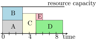
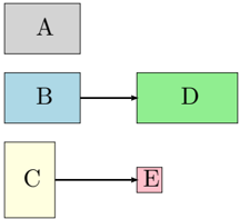
Example 1.1. Consider a simple cumulative resource scheduling problem. There are 5 activities A, B, C, D, and E to be executed before time period 10. The activities have processing times 3, 3, 2, 4, and 1, respectively, with each activity requiring 2, 2, 3, 2, and 1 units of resource, respectively. There is a resource capacity of 4. Assume further that there are precedence constraints: activity B must finish before activity D begins, written B glyph[lessmuch] D , and similarly C glyph[lessmuch] E . Figure 1 shows the five activities and precedence relations, while Fig. 2 shows a possible schedule, where the start times are: 0, 0, 3, 5, and 5 respectively.

In Cp solvers, a cumulative resource constraint can be modelled by a decomposition or, more successfully, by the global constraint cumulative [2]. Since the introduction of this global constraint, a great deal of research has investigated stronger and faster propagation techniques. These include time-table [2], (extended) edge-finding [21, 33], not-first/not-last [21, 25], and energetic-reasoning propagation [4, 6]. Time-table propagation is usually superior for highly disjunctive problems, i.e. , in which only some activities can run concurrently, while (extended) edge-finding, not-first/not-last, and energetic reasoning are more appropriate for highly cumulative problems, i.e. , in which many activities can run concurrently.[4] The reader is referred to [6] for a detailed comparison of these techniques.

Vilim [34] recently developed TtEf propagation which combines the time-table and (extended) edge-finding propagation in order to perform stronger propagation while having a low runtime overhead. Vilim [34] shows that on a range of highly disjunctive open resource-constrained project scheduling problems from the well-established benchmark

library PSPLib, 1 TtEf propagation can generate lower bounds on the project deadline ( makespan ) that are superior to those found by previous methods. He uses a Cp solver without nogood learning. This result, and the success of Lcg on such problems, motivated us to study whether an explaining version of this propagation yields an improvement in performance for Lcg solvers.

In general, nogood learning is a resolution step that infers redundant constraints, called nogoods , given an inconsistent solution state. These nogoods are permanently or temporarily added to the initial constraint system in order to reduce the search space and/or to guide the search. Moreover, they can be used to short circuit propagation. How this resolution step is performed is dependent on the underlying system.

Lcg solvers employ a 'fine-grained' nogood learning system that mimics the learning of modern Boolean satisfiability ( Sat ) solvers (see e.g. [20]). In order to create a strong nogood, it is necessary that each inconsistency and value removal is explained concisely and in the most general way possible. For Lcg solvers, we have previously developed explanations for time-table and (extended) edge-finding propagation [27]. Moreover, for time-table propagation we have also considered the case when processing times, resource usages, and resource capacity are variable [24]. Explanations for the time-table propagator were successfully applied on resource-constraint project scheduling problems [27, 29] and carpet cutting [28] where in both cases the state-of-the-art of exact solution methods were substantially improved. The explanations defined here are similar to the step-wise ones for the (extended) edge-finding propagation in [27], but there we do not consider the resource profile and are more complex. Moreover, the proposed explanations for edge-finding propagation in [27] has never been implemented.

Explanations for the propagation of the cumulative constraint have also been proposed for the PaLM [14, 13] and SCIP [1, 7, 12] frameworks. In the PaLM framework, explanations are only considered for time-table propagation, while the SCIP framework additionally provides explanations for energetic reasoning propagation and a restricted version of edge-finding propagation. Neither framework consider bounds widening in order to generalise these explanations as we do in this paper. Other related works include [32], which presents explanations for different propagation techniques for problems only involving disjunctive resources, i.e. , cumulative resources with unary resource capacity, and generalised nogoods [15]. A detailed comparison of explanations for the propagation of cumulative resource constraints in Lcg solvers can be found in [24].

In this paper we develop explanations for the TtEf cumulative propagator in Lcg solvers. The explaining TtEf propagation is then compared with the explaining timetable propagation from [27] in the Lcg solver on Rcpsp using the reengineered Lcg solver [9] which was also used for the experiments presented in [27].

2. Cumulative Resource Scheduling

In cumulative resource scheduling, a set of (non-preemptive) activities V and one cumulative resource with a (constant) resource capacity R is given where an activity i is

1 See http://129.187.106.231/psplib/ .

specified by its start time S i , its processing time p i , its resource usage r i , and its energy e i := p i · r i . In this paper we assume each S i is an integer variable and all others are assumed to be integer constants. Further, we define est i ( ect i ) and lst i ( lct i ) as the earliest and latest start (completion) time of i .

In this setting. the cumulative resource scheduling problem is defined as a constraint satisfaction problem that is characterised by the set of activities V and a cumulative resource with resource capacity R . The goal is to find a solution that assigns values from the domain to the start time variables S i ( i ∈ V ), so that the following conditions are satisfied.

where τ ranges over the time periods considered. Note that this problem is NP-hard [5].

We shall tackle problems including cumulative resource scheduling using Cp with nogood learning. In a Cp solver, each variable S i , i ∈ V has an initial domain of possible values D 0 ( S i ) which is initially [ est i , lst i ]. The solver maintains a current domain D for all variables. Cp search interleaves propagation with search. The constraints are represented by propagators that, given the current domain D , creates a new smaller domain D ′ by eliminating infeasible values. The current lower and upper bound of the domain D ( S i ) are denoted by lb ( S i ) and ub ( S i ), respectively. For more details on Cp see e.g. [23].

For a learning solver we also represent the domain of each variable S i using Boolean variables J S i ≤ v K , est i ≤ v < lst i . These are used to track the reasons for propagation and generate nogoods. For more details see [22]. We use the notation J v ≤ S i K , est i < v ≤ lst i as shorthand for ¬ J S i ≤ v -1 K , and treat J v ≤ S i K , v ≤ est i and J S i ≤ v K , v ≥ lst i as synonyms for true . Propagators in a learning solver must explain each reduction in the domain by building a clausal explanation using these Boolean variables.

Optimisation problems are typically solved in Cp via branch and bound. Given an objective obj which is to be minimised, when a solution is found with objective value o , a new constraint obj < o is posted to enforce that we only look for better solutions in the subsequent search.

3. TTEF Propagation

In this section we develop explanations for TtEf propagation. For a more detailed description about TtEf propagation the reader is referred to [34].

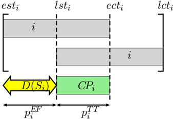
TtEf propagation splits the treatment of activities into a fixed and free part. The former results from the activities' compulsory part whereas the latter is the remainder. The fixed part of an activity i is characterised by the length of its compulsory part p TT i := max(0 , ect i -lst i ) and its fixed energy e TT i := r i · p TT i . The free part has a processing time p EF i := p i -p TT i and a free energy of e EF i := e i -e EF i . Let V EF be the set of

activities with a non-empty free part { i ∈ V | p EF i > 0 } . An illustration of this is shown in Figure 3.

TtEf propagation reasons about the energy available from the resource and energy required for the execution of activities in specific time windows. The start and end times of these windows are determined by the earliest start and the latest completion times of activities i ∈ V EF . These time windows [ begin, end ) are characterised by the so-called task intervals V EF ( a, b ) := { i ∈ V EF | est a ≤ est i ∧ lct i ≤ lct b } where a, b ∈ V EF , begin := est a , and end := lct b .

It is not only the free energy of activities in the task interval V EF ( a, b ) that is considered, but also the energy resulting from the compulsory parts in the time window [ est b , lct b ). This energy is defined by ttEn ( a, b ) := ttAfter [ est a ] -ttAfter [ lct b ] where ttAfter [ τ ] := ∑ t ≥ τ ∑ i ∈V : lst i ≤ t<ect i r i .

Furthermore, we also consider activities i ∈ V \ V EF ( a, b ) in which a portion of their free part must be run within the time window as described in [34]. Let lst EF i be the latest start time of the free part of an activity, i.e. , lct i -p EF i . Then activity i 's free part consumes at least r i · ( lct b -lst EF i ) energy units in [ est a , lct b ) if est a ≤ est i and lst EF i < lct b . We define the energy contributed by such activities by rsEn ( a, b ) := ∑ i ∈V\V EF ( a,b ): est a ≤ est i max (0 , lct b -lst EF i ).

In summary, TtEf propagation considers three ways in which an activity i can contribute to energy consumption within a time window determined by a task interval V EF ( a, b ). First, the free parts that must fully be executed in the time window; second, the compulsory parts that must lies in the time window; and third, some free parts that must partially be run in the time window. Thus, the considered length of an activity i is

The considered energy consumption is e i ( a, b ) := r i · p i ( a, b ) in the time window.

3.1. Explanation for the TTEF Consistency Check

The consistency check is one part of TtEf propagation that checks whether there is a resource overload in any task interval.

Proposition 3.1 (Consistency Check) . The cumulative resource scheduling problem is inconsistent if

This check can be done in O ( l 2 + n ) runtime, where l = |V EF | , if the resource profile is given. The corresponding algorithm is shown in Alg. 1 in App. A.

A na¨ ıve explanation for a resource overload in the time window [ est a , lct b ) only considers the current bounds on activities' start times S i .

However, we can easily generalise this explanation by only ensuring that at least p i ( a, b ) time units are executed in the time window. This results in the following explanation.

Note that this explanation expresses a resource overload with respect to energetic reasoning propagation which is more general than TtEf .

Let ∆ := energy ( a, b ) -R · ( lct b -est a ) -1. If ∆ > 0 then the resource overload has extra energy. We can use this extra energy to further generalise the explanation, by reducing the energy required to appear in the time window by up to ∆. For example, if r i ≤ ∆ then the lower and upper bound on S i can simultaneously be decreased and increased by a total amount in { 1 , 2 , ..., min( glyph[floorleft] ∆ /r i glyph[floorright] , p i ( a, b )) } units without resolving the overload. If r i · p i ( a, b ) ≤ ∆ then we can remove activity i completely from the explanation. In a greedy manner, we try to maximally widen the bounds of activities i where p i ( a, b ) > 0, first considering activities with non-empty free parts. If ∆ i denotes the time units of the widening then it holds p i ( a, b ) ≥ ∆ i ≥ 0 and ∑ i ∈V : p i ( a,b ) > 0 ∆ i · r i ≤ ∆ and we create the following explanation.

The last generalisation mechanism can be performed in different ways, e.g. we could widen the bounds of activities that were involved in many recent conflicts. Further study is required to identify which are the most appropriate.

3.2. Explanation for the TTEF Start Times Propagation

Propagation on the lower and upper bounds of the start time variables S i are symmetric; Consequently we only present the case for the lower bounds' propagation. To prune the lower bound of an activity u , TtEf bounds propagation tentatively starts the activity u at its earliest start time est u and then checks whether that causes a resource overload in any time window [ est a , lct b ) ( { a, b } ⊆ V EF ). Thus, bounds propagation and its explanation are very similar to that of the consistency check.

The work of [34] considers four positions of u relative to the time window: right ( est a ≤ est u < lct b < ect u ), inside ( est a ≤ est u < ect u ≤ lct b ), through ( est u < est a ∧ lct b < ect u ), and left ( est u < est a < ect u ≤ lct b ). The first two of these positions correspond to edge-finding propagation and the last two to extended edge-finding propagation. We first consider only the right and inside positions, i.e. , est a ≤ est u . Note that a could be u . Then,

where energy ( a, b, u ) := energy ( a, b ) -e u ( a, b ) + r u · (min( lct b , ect u ) -est u ) and

The first two terms in the sum of energy ( a, b, u ) gives the energy consumption of all considered activities except u , whereas the last term is the required energy of u if it is scheduled at est u in the time window [ est a , lct b ). The propagation, including explanation generation, can be performed in O ( l 2 + k · n ) runtime, where l = |V EF | and k the number of bounds' updates, if the resource profile is given. Moreover, TtEf propation does not necessarily consider each u ∈ V EF , but those only that maximise min( e EF u , r u · ( lct b -est a )) -r u · max(0 , lct b -lst EF u ) and satisfy est a ≤ est u . The corresponding algorithm is shown in Alg. 2 in App. A.

Ana¨ ıve explanation for a lower bound update from est u to newLB := glyph[ceilingleft] rest ( a, b, u ) /r u glyph[ceilingright] with respect to the time window [ est a , lct b ) additionally includes the previous and new lower bound on the left and right hand side of the implication, respectively, in comparison to the na¨ ıve explanation for a resource overload.

As we discussed in the case of resource overload, we perform a similar generalisation for the activities in V \ { u } , and for u we decrease the lower bound on the left hand side as much as possible so that the same propagation holds when u is executed at that

Table 1: Specifications of the benchmark suites.

suite	sub-suites	#inst	#act	p i	#res	notes
AT [3]	st 27/ st 51/ st 103	48 each	25/49/101	1-12	6 each
PSPLib [16]	j30 [17]/ j60 / j90 j120	480 each 600	30/60/90 30	1-10 1-10	4 each 4
BL [4]	bl 20/ bl 25	20 each	20/25	1-6	3 each
Pack [8]		55	15-33	1-19	2-5
KSD15 d [18]		480	15	1-250	4	based on j30
Pack d [18]		55	15-33	1-1138	2-5	based on Pack

decreased lower bound.

Again this more general explanation expresses the energetic reasoning propagation and the bounds of activities in { i ∈ V \ { u } | p i ( a, b ) > 0 } can further be generalised in the same way as for a resource overload. But here the available energy units ∆ for widening the bounds is rest ( a, b, u ) -r u · ( newLB -1) + 1. Hence, 0 ≤ ∆ < r u indicate that the explanation only can further be generalised a little bit. We perform this generalisation as for the overload case.

4. Experiments on Resource-constrained Project Scheduling Problems

We carried out extensive experiments on Rcpsp instances comparing our solution approach using both time-table and/or TtEf propagation. We compare the obtained results on the lower bounds of the makespan with the best known so far. Detailed results are available at http://www.cs.mu.oz.au/ ~ pjs/rcpsp .

We used six benchmark suites for which an overview is given in Tab. 1 where #inst, #act, p i , and #res are the number of instances, number of activities, range of processing times, and number of resources, respectively. The first two suites are highly disjunctive, while the remainder are highly cumulative.

The experiments were run on a X86-64 architecture running GNU/Linux and a Intel(R) Core(TM) i7 CPU processor at 2.8GHz. The code was written in Mercury [30] using the G12 Constraint Programming Platform [31].

We model an instance as in [27] using global cumulative constraints cumulative and difference logic constraints ( S i + p i ≤ S j ), resp. In addition, between two activities i , j in disjunction, i.e. , two activities which cannot concurrently run without overloading some

resource, the two half-reified constraints [10] b → S i + p i ≤ S j and ¬ b → S j + p j ≤ S i are posted where b is a Boolean variable.

We run cumulative constraint propagation using different phases:

• (a) time-table consistency check in O ( n + p log p ) runtime,
• (b) TtEf consistency check in O ( l 2 + n ) runtime as defined in Section 3.1,
• (c) time-table bounds' propagation in O ( l · p + k · min( R,n )) runtime, and
• (d) TtEf bounds' propagation in O ( l 2 + k · n ) runtime as defined in Section 3.2 where k, l, n, p are the numbers of bounds' updates, unfixed activities, all activities, and height changes in the resource profile, resp.

Note that in our setup phase (d) TtEf bounds' propagation does not take into account the bounds' changes of the phase (c) time-table bounds' propagation. For the experiments, we consider three settings of the cumulative propagator: tt executes phases (a) and (c), ttef(c) (a-c), and ttef (a-d). Note that phases (c) and (d) are not run if either phase (a) or (b) detects inconsistency.

4.1. Upper Bound Computation

For solving Rcpsp we use the same branch-and-bound algorithm as we used in [27], but here we limit ourselves to the search heuristic HotRestart which was the most robust one in our previous studies [26, 27]. It executes an adapted search of [4] using serial scheduling generation for the first 500 choice points and, then, continues with an activity based search (a variant of Vsids [20]) on the Boolean variables representing a lower part x ≤ v and upper part v < x of the variable x 's domain where x is either a start time or the makespan variable and v a value of x 's initial domain. Moreover, it is interleaved with a geometric restart policy [35] on the number of node failures for which the restart base and factor are 250 failures and 2.0, respectively. The search was halted after 10 minutes.

The results are given in Tab. 2 and 3. For each benchmark suite, the number of solved instances (#svd) is given. The column cmpr( a ) shows the results on the instances solved by all methods, where a is the number of such instances. The left entry in that column is the average runtime on these instances in seconds, and the right entry is the average number of failures during search. The entries in column all( a ) have the same meaning, but here all instances are considered where a is the total number of instances. For unsolved instances, the number of failures after 10 minutes is used.

Table 2 shows the results on the highly disjunctive Rcpsp s. As expected, the stronger propagation ( ttef(c) , ttef ) reduces the search space overall in comparision to tt , but the average runtime is higher by a factor of about 5%-70% and 50%-100% for ttef(c) and ttef . Interestingly, ttef(c) and ttef solved respectively 1 and 2 more instances on j60 and closed the instance j120 1 1 on j120 which has an optimal makespan 105. This makespan corresponds to the best known upper bound. However, the stronger propagation does not generally pay off for a Cp solver with nogood learning.

Table 2: UB results on highly disjunctive Rcpsp s.

	j30
	#svd	cmpr(480)		all(480)		#svd	cmpr(429)		all(480)
tt	480	0.12	1074	0.12	1074	430	1.82	5798	64.25	93164
ttef(c)	480	0.20	1103	0.20	1103	431	2.00	4860	64.39	80845
ttef	480	0.23	991	0.23	991	432	3.04	5191	64.87	62534
	j90					j120
	#svd	cmpr(400)		all(480)		#svd	cmpr(280)		all(600)
tt	400	5.03	9229	104.09	132234	283	9.71	15022	322.35	398941
ttef(c)	400	6.93	9512	105.69	104297	282	13.47	16958	324.73	297562
ttef	400	8.10	8830	106.66	72402	283	14.97	13490	324.66	186597
	AT
	#svd	cmpr(129)		all(144)
tt	132	8.90	19997	66.22	87226
ttef(c)	130	9.36	16466	69.41	72056
ttef	129	13.55	17239	74.60	63554

Table 3: UB results on highly cumulative Rcpsp s.

	BL					Pack
	#svd	cmpr(40)		all(40)		#svd	cmpr(16)		all(55)
tt	40	0.16	2568	0.16	2568	16	77.65	245441	447.69	699615
ttef(c)	40	0.02	370	0.02	370	39	37.22	122038	186.79	292101
ttef	40	0.02	269	0.02	269	39	44.44	105751	188.23	257747
	KSD15 d					Pack d
	#svd	cmpr(480)		all(480)		#svd	cmpr(37)		all(55)
tt	480	0.01	26	0.01	26	37	32.72	42503	218.26	184293
ttef(c)	480	0.01	26	0.01	26	37	23.96	32916	212.37	170301
ttef	480	0.01	26	0.01	26	37	36.93	37004	221.11	157015

Table 4: LB results on AT , Pack , and Pack d

	AT	Pack	Pack d
ttef(c)	5/4/3 +52	0/4/12 +100	0/7/11 +632
ttef	7/2/3 +44	1/4/11 +101	2/5/10 +618

Table 5: LB results on j60 , j90 , and j120

		j60			j90					j120
		+1 +2		+3	+1	+2	+3	+4	+5	+1	+2	+3	+4	+5	+6	+7	+8	+9	+10
1 min	ttef(c)	4	1	-	12	1	-	-	-	27	8	4	-	-	-	2	-	-	-
	ttef	7	5	-	25	14	3	1	-	90	20	10	5	2	-	-	2	-	-
	ttef(c)	21	2	-	25	7	-	-	-	68	16	4	4	2	-	-	1	1	-
	ttef	13	6	3	35	17	6	3	1	116	39	9	9	4	1	-	-	1	1

Table 3 presents the results on highly cumulative Rcpsp s which clearly shows the benefit of TtEf propagation, especially on BL for which ttef(c) and ttef reduce the search space and the average runtime by a factor of 8, and Pack for which they solved 23 instances more than tt . On Pack d , ttef(c) is about 50% faster on average than tt while ttef is slightly slower on average than tt . No conclusion can be drawn on KSD15 d because the instances are easy for Lcg solvers.

4.2. Lower Bound Computation

The lower bound computation tries to solve Rcpsp s in a destructive way by converging to the optimal makespan from below, i.e. , it repeatedly proves that there exists no solution for current makespan considered and continues with an incremented makespan by 1. If a solution found then it is the optimal one. For these experiments we use the search heuristic HotStart as we did in [26, 27]. This heuristic is HotRestart (as decribed earlier) but no restart. We used the same parameters as for HotRestart . For the starting makespan , we choose the best known lower bounds on j60 , j90 , and j120 recorded in the PSPLib at http://129.187.106.231/psplib/ and [34] at http:// vilim.eu/petr/cpaior2011-results.txt . On the other suites, the search starts from makespan 1. Due to the tighter makespan , it is expected that the TtEf propagation will perform better than for upper bound computation on the highly disjunctive instances. The search was cut off at 10 minutes as in [26, 27].

Table 4 shows the results on AT , Pack , and Pack d restricted to the instances that none of the methods could solve using the upper bound computation, that are 12, 16, and 18 for AT , Pack , and Pack d , respectively. An entry a / b / c for method x means that x achieved respectively a -times, b -times and c -times a worse, the same and a better lower bound than tt . The entry + d is the sum of lower bounds' differences of method x to tt . On Pack and Pack d , ttef(c) and ttef clearly perform better than tt . On the highly disjunctive instances in AT , ttef(c) and tt are almost balanced whereas tt could generate better lower bounds on more instances as ttef . The lower bounds' differences on AT are dominated by the instance st103 4 for which ttef(c) and ttef retrieved a lower

bound improvement of 54 and 53 time periods with respect to tt .

The more interesting results are presented in Tab. 5 because the best lower bounds are known for all the remaining open instances (48, 77, 307 in j60 , j90 , j120 ). 2 An entry in a column + d shows the number of instances for that the corresponding method could improve the lower bound by d time periods. On these instances, we run at first the experiments with a runtime limit of one minute as it was done in the experiments for TtEf propagation in [34] but he used a Cp solver without nogood learning. tt could not improve any lower bound because its corresponding results are already recorded in the PSPLib. ttef(c) and ttef improved the lower bounds of 59 and 183 instances, respectively, which is about 13.7% and 42.4% of the open instances. Although, the experiments in [34] were run on a slower machine 3 the results confirm the importance of nogood learning. For the experiments with 10 minutes runtime, we excluded tt due to time constraints and expected inferior results to ttef(c) and ttef . With the extended runtime, ttef(c) and ttef could improved the lower bounds of more instance, namely 151 and 264 instances, respectively, which is about 35.0% and 61.1%. Moreover, 3, 1, and 1 of the remaining open instances on j60 , j90 , and j120 , respectively, could be solved optimally. See App. B for the listing of the closed instances and the new lower bounds.

5. Conclusion and Outlook

We present explanations for the recently developed TtEf propagation of the global cumulative constraint for lazy clause generation solvers. These explanations express an energetic reasoning propagation which is a stronger propagation than the TtEf one.

Our implementation of this propagator was compared to time-table propagation in lazy clause generation solvers on six benchmark suites. The preliminary results confirms the importance of energy-based reasoning on highly disjunctive Rcpsp s for Cp solvers with nogood learning.

Moreover, our approach with TtEf propagation was able to close one instance. It also improves the best known lower bounds for 264 of the remaining 432 remaining open instances on Rcpsp s from the PSPLib.

In the future, we want to integrate the extended edge-finding propagation into TtEf propagation as it was originally proposed in [34], to perform experiments on cutting and packing problems, and to study different variations of explanations for TtEf propagation. Furthermore, we want to look at a more efficient implementation of the TtEf propagation as well as an implementation of energetic reasoning.

Acknowledgements NICTA is funded by the Australian Government as represented by the Department of Broadband, Communications and the Digital Economy and the Australian Research Council through the ICT Centre of Excellence program. This work

2 Note that the PSPLib still lists the instances j60 25 5 , j90 26 5 , j120 8 3 , j120 48 5 , and j120 35 5 as open, but we closed the first four ones in [27] and [19] closed the last one.

3 Intel(R) Core(TM)2 Duo CPU T9400 on 2.53GHz

was partially supported by Asian Office of Aerospace Research and Development grant 10-4123.

References

1. Tobias Achterberg. SCIP: solving constraint integer programs. Mathematical Programming Computation , 1:1-41, 2009. ISSN 1867-2949. doi: 10.1007/ s12532-008-0001-1.
2. Abderrahmane Aggoun and Nicolas Beldiceanu. Extending CHIP in order to solve complex scheduling and placement problems. Mathematical and Computer Modelling , 17(7):57-73, 1993.
3. Ram´ on Alvarez-Vald´ es and Jos´ e Manuel Tamarit. Advances in Project Scheduling , chapter Heuristic algorithms for resource-constrained project scheduling: A review and an empirical analysis, pages 113-134. Elsevier, 1989.
4. Philippe Baptiste and Claude Le Pape. Constraint propagation and decomposition techniques for highly disjunctive and highly cumulative project scheduling problems. Constraints , 5(1-2):119-139, 2000.
5. Philippe Baptiste, Claude Le Pape, and Wim Nuijten. Satisfiability tests and timebound adjustments for cumulative scheduling problems. Annals of Operations Research , 92:305-333, 1999. doi: 10.1023/A:1018995000688.
6. Philippe Baptiste, Claude Le Pape, and Wim Nuijten. Constraint-Based Scheduling . Kluwer Academic Publishers, Norwell, MA, USA, 2001. ISBN 0792374088.
7. Timo Berthold, Stefan Heinz, Marco L¨ ubbecke, Rolf M¨ ohring, and Jens Schulz. A constraint integer programming approach for resource-constrained project scheduling. In Andrea Lodi, Michela Milano, and Paolo Toth, editors, Integration of AI and OR Techniques in Constraint Programming for Combinatorial Optimization Problems , volume 6140 of Lecture Notes in Computer Science , pages 313-317. Springer Berlin / Heidelberg, 2010. doi: 10.1007/978-3-642-13520-0 34.
8. Jacques Carlier and Emmanuel N´ eron. On linear lower bounds for the resource constrained project scheduling problem. European Journal of Operational Research , 149(2):314-324, 2003. ISSN 0377-2217. doi: 10.1016/S0377-2217(02)00763-4.
9. Thibaut Feydy and Peter J. Stuckey. Lazy clause generation reengineered. In Gent [11], pages 352-366. doi: 10.1007/978-3-642-04244-7 29.
10. Thibaut Feydy, Zoltan Somogyi, and Peter J. Stuckey. Half reification and flattening. In Jimmy Ho-Man Lee, editor, Proceedings of Principles and Practice of Constraint Programming - CP 2011 , volume 6876 of Lecture Notes in Computer Science , pages 286-301. Springer, 2011.

1. Ian P. Gent, editor. Proceedings of Principles and Practice of Constraint Programming - CP 2009 , volume 5732 of Lecture Notes in Computer Science , 2009. Springer Berlin / Heidelberg.
2. Stefan Heinz and Jens Schulz. Explanations for the cumulative constraint: An experimental study. In Panos M. Pardalos and Steffen Rebennack, editors, Proceedings of Experimental Algorithms - SEA 2011 , volume 6630 of Lecture Notes in Computer Science , pages 400-409. Springer Berlin / Heidelberg, 2011. doi: 10.1007/978-3-642-20662-7 34.
3. Narendra Jussien. The versatility of using explanations within constraint programming. Research Report 03-04-INFO, ´ Ecole des Mines de Nantes, Nantes, France, 2003.
4. Narendra Jussien and Vincent Barichard. The PaLM system: explanation-based constraint programming. In Proceedings of TRICS: Techniques foR Implementing Constraint programming Systems, a post-conference workshop of CP 2000 , pages 118-133, Singapore, 2000.
5. George Katsirelos and Fahiem Bacchus. Generalized nogoods in CSPs. In Manuela M. Veloso and Subbarao Kambhampati, editors, Proceedings on Artificial Intelligence - AAAI 2005 , pages 390-396. AAAI Press / The MIT Press, 2005.
6. Rainer Kolisch and Arno Sprecher. PSPLIB - A project scheduling problem library. European Journal of Operational Research , 96(1):205-216, 1997. doi: 10.1016/ S0377-2217(96)00170-1.
7. Rainer Kolisch, Arno Sprecher, and Andreas Drexl. Characterization and generation of a general class of resource-constrained project scheduling problems. Management Science , 41(10):1693-1703, 1995. ISSN 0025-1909.
8. Oumar Kon´ e, Christian Artigues, Pierre Lopez, and Marcel Mongeau. Event-based milp models for resource-constrained project scheduling problems. Computers & Operations Research , 38(1):3-13, 2011. doi: 10.1016/j.cor.2009.12.011.
9. Olivier Liess and Philippe Michelon. A constraint programming approach for the resource-constrained project scheduling problem. Annals of Operations Research , 157(1):25-36, January 2008. doi: 10.1007/s10479-007-0188-y.
10. Matthew W. Moskewicz, Conor F. Madigan, Ying Zhao, Lintao Zhang, and Sharad Malik. Chaff: Engineering an efficient SAT solver. In Proceedings of Design Automation Conference - DAC 2001 , pages 530-535, New York, NY, USA, 2001. ACM. doi: 10.1145/378239.379017.
11. Wilhelmus Petronella Maria Nuijten. Time and Resource Constrained Scheduling . PhD thesis, Eindhoven University of Technology, 1994.

1. Olga Ohrimenko, Peter J. Stuckey, and Michael Codish. Propagation via lazy clause generation. Constraints , 14(3):357-391, 2009.
2. Christian Schulte and Peter J. Stuckey. Efficient constraint propagation engines. ACM Transactions on Programming Languages and Systems , 31(1):Article No. 2, 2008.
3. Andreas Schutt. Improving Scheduling by Learning . PhD thesis, The University of Melbourne, 2011. URL http://repository.unimelb.edu.au/10187/11060 .
4. Andreas Schutt and Armin Wolf. A new O ( n 2 log n ) not-first/not-last pruning algorithm for cumulative resource constraints. In David Cohen, editor, Proceedings of Principles and Practice of Constraint Programming - CP 2010 , volume 6308 of Lecture Notes in Computer Science , pages 445-459. Springer Berlin / Heidelberg, 2010. URL 10.1007/978-3-642-15396-9_36 .
5. Andreas Schutt, Thibaut Feydy, Peter J. Stuckey, and Mark G. Wallace. Why cumulative decomposition is not as bad as it sounds. In Gent [11], pages 746-761. doi: 10.1007/978-3-642-04244-7 58.
6. Andreas Schutt, Thibaut Feydy, Peter J. Stuckey, and Mark G. Wallace. Explaining the cumulative propagator. Constraints , 16(3):250-282, 2011. doi: 10.1007/s10601-010-9103-2.
7. Andreas Schutt, Peter Stuckey, and Andrew Verden. Optimal carpet cutting. In Jimmy Lee, editor, Principles and Practice of Constraint Programming - CP 2011 , volume 6876 of Lecture Notes in Computer Science , pages 69-84. Springer Berlin / Heidelberg, 2011. doi: 10.1007/978-3-642-23786-7 8.
8. Andreas Schutt, Thibaut Feydy, Peter J. Stuckey, and Mark G. Wallace. Solving RCPSP/max by lazy clause generation. Journal of Scheduling , pages 1-18, 2012. doi: 10.1007/s10951-012-0285-x.
9. Zoltan Somogyi, Fergus Henderson, and Thomas Conway. The execution algorithm of Mercury, an efficient purely declarative logic programming language. The Journal of Logic Programming , 29(1-3):17-64, 1996. ISSN 0743-1066. doi: 10.1016/S0743-1066(96)00068-4.
10. Peter J. Stuckey, Maria J. Garc´ ıa de la Banda, Michael J. Maher, Kim Marriott, John K. Slaney, Zoltan Somogyi, Mark G. Wallace, and Toby Walsh. The G12 project: Mapping solver independent models to efficient solutions. In Maurizio Gabbrielli and Gopal Gupta, editors, Proceedings of Logic Programming - ICLP 2005 , volume 3668 of Lecture Notes in Computer Science , pages 9-13. Springer Berlin / Heidelberg, October 2005. doi: 10.1007/11562931 3.
11. Petr Vil´ ım. Computing explanations for the unary resource constraint. In Roman Bart´ ak and Michela Milano, editors, Proceedings of Integration of AI and OR

Techniques in Constraint Programming for Combinatorial Optimization Problems CPAIOR 2005 , volume 3524 of Lecture Notes in Computer Science , pages 396-409. Springer Berlin / Heidelberg, 2005. doi: 10.1007/11493853 29.

1. Petr Vil´ ım. Edge finding filtering algorithm for discrete cumulative resources in O ( kn log n ). In Gent [11], pages 802-816. doi: 10.1007/978-3-642-04244-7 62.
2. Petr Vil´ ım. Timetable edge finding filtering algorithm for discrete cumulative resources. In Tobias Achterberg and J. Beck, editors, Proceedings of Integration of AI and OR Techniques in Constraint Programming for Combinatorial Optimization Problems - CPAIOR 2011 , volume 6697 of Lecture Notes in Computer Science , pages 230-245. Springer Berlin / Heidelberg, 2011. doi: 10.1007/ 978-3-642-21311-3 22.
3. Toby Walsh. Search in a small world. In Proceedings of Artificial intelligence IJCAI 1999 , pages 1172-1177. Morgan Kaufmann, 1999.

A. TTEF propagation algorithms

Algorithm 1 shows the TtEf consistency check used. The outer loop (lines 2-16) iterates over all distinctive possible end times for the time windows while the inner loop (lines 7-16) iterates over all possible start times. In line 11 (12), it checks whether a must fully (partially) be executed in the current time window and further ones checked in the same inner loop. If so it adds the required free energy units e EF a of a to E . In line 13, it calculates the still available energy units in the time window [ begin, end ) taking the energy units from the resource profile ttEn ( a, b ) into account. If this results in a resource overload then a corresponding explanation is generated (line 15) and the algorithm fails; otherwise, the algorithm succeeds.

Algorithm 1: TtEf consistency check.

Input : X an array of activities sorted in non-decreasing order of the earliest start time. Input : Y an array of activities sorted in non-decreasing order of the latest completion time. 1 end = ∞ ; 2 for y := n down to 1 do 3 b := Y [ y ]; 4 if lct b = end then continue; 5 end := lct b ; 6 E := 0; 7 for x := n down to 1 do 8 a := X [ x ]; 9 if end ≤ est a then continue; 10 begin := est a ; 11 if lct a ≤ end then E := E + e EF a ; 12 if lst EF a < end then E := E + r a · ( end -lst EF a ); 13 avail := R · ( end -begin ) -E -ttEn ( a, b ); 14 if avail < 0 then 15 explainOverload( begin , end ); 16 return false ; 17 return true ;

Algorithm 2 shows the lower bounds propagation algorithm. As for Alg. 1 the outer loop (lines 3-24) and inner loop (lines 7-24) iterate over the end and start times of the time windows [ begin, end ), but require more book keeping. In line 6, it initialises E . u , and enReqU where: E records the required energy units by the considered activities that must fully or partially be run in the time window; and u stores the activity that maximises min( e EF u , r u · ( end -begin )) -r u · max(0 , end -lst EF u ) and that value is saved in enReqU . If a must be fully or partially be executed in the time window then the corresponding energy units are added to E in lines 11 and 14, resp. The desired activity for pruning is computed in lines 13, 15, and 16, whereas the available energy units are calculated in line 17. In the case that there is not sufficient energy available then the condition of line 18 holds and the algorithm determines the first possible start time for u (lines 19, 20). If that is larger than the recorded earliest start time in est ′ u then the algorithm generates the explanation (line 22) and postpones the update (line 23) after finishing with the outer loop (line 25).

Algorithm 2: TtEf lower bounds propagator on the start times. Input : X an array of activities sorted in non-decreasing order of the earliest start time. Input : Y an array of activities sorted in non-decreasing order of the latest completion time. 1 for i ∈ V EF do est ′ i := est i ; 2 end := ∞ ; k := 0; 3 for y := n down to 1 do 4 b := Y [ y ]; 5 if lct b = end then continue; 6 end := lct b ; E := 0; u := -∞ ; enReqU := 0; 7 for x := n down to 1 do 8 a := X [ x ]; 9 if end ≤ est a then continue; 10 begin := est a ; 11 if lct a ≤ end then E := E + e EF a ; 12 else 13 enIn := r a · max(0 , end -lst EF a ); 14 E := E + enIn ; 15 enReqA := min( e EF a , r a · ( end -est a )) -enIn ; 16 if enReqA > enReqU then u := a ; enReqU := enReqA ; 17 avail := R · ( end -begin ) -E -ttEn ( a, b ); 18 if enReqU > 0 and avail -enReqU < 0 then 19 rest := E -avail -r a · max(0 , end -lst a ); 20 lbU := begin + glyph[ceilingleft] rest/r u glyph[ceilingright] ; 21 if est ′ u < lbU then 22 expl := explainUpdate ( begin, end, u, est ′ u , lbU ); 23 Update [++ k ] := ( u, lbU, expl ); 24 est ′ u := lbU ; 25 for z := 1 to k do updateLB ( Update [ z ]);

Table 6: New lower bounds on j60 .

inst	LB	inst	LB	inst	LB	inst	LB	inst	LB	inst	LB	inst	LB
9 1	85	9 5	81	9 6	106	9 7	103	9 8	95	9 10	89	13 1	105
13 2	103	13 3	84	13 4	98	13 7	82	13 8	115	13 9	96	13 10	113
25 2	96	25 4	106	25 6	106	29 1	97	29 6	144	29 7	115	29 8	97
41 3	90	41 10	106	45 1	90

Table 7: New lower bounds on j90 .

inst	LB	inst	LB	inst	LB	inst	LB	inst	LB	inst	LB	inst	LB
5 3	84	5 5	109	5 7	106	5 8	97	5 9	114	5 10	95	9 2	122
9 3	98	9 4	120	9 5	127	9 6	113	9 7	103	9 8	111	9 9	106
9 10	105	13 2	119	13 3	105	13 5	109	13 7	116	13 8	113	13 9	117
13 10	114	21 7	106	21 8	108	25 1	117	25 2	122	25 3	113	25 4	128
25 5	110	25 6	113	25 8	131	25 9	98	25 10	119	29 1	126	29 2	122
29 4	139	29 6	117	29 7	160	29 8	146	29 9	120	30 9	92	37 2	114
41 1	129	41 2	154	41 3	149	41 4	142	41 5	116	41 6	124	41 7	145
41 8	148	41 9	110	41 10	144	45 1	143	45 2	138	45 3	144	45 4	126
45 6	163	45 7	129	45 8	150	45 9	145	45 10	156	46 9	86

B. Closed Instances and New Lower Bounds on PSPLib

From the open instances, we closed the instances 9 3 (100), 9 9 (99), 25 10 (108) on j60 , 5 6 (86) on j90 , and 1 1 (105), 8 6 (85) on j120 where the number in brackets shows the optimal makespan. We computed new lower bounds on the remaining open instances from the PSPLib. Tables 6-8 list these new lower bounds where the column 'inst' shows the name of the instance and the column 'LB' the corresponding new lower bound.

C. Best Lower and Upper Bounds Retrieved

For a later comparison, Tables 9-11 show the best lower and upper bounds for AT , Pack , and Pack d retrieved by one of the methods tt , ttef(c) , and ttef . The column 'inst' shows the instance name and the column 'LB/UB' the corresponding lower and upper bound. If these bounds are equal then only one number is given.

Table 8: New lower bounds on j120 .

inst	LB	inst	LB	inst	LB	inst	LB	inst	LB	inst	LB	inst	LB
6 1	134	6 2	127	6 5	117	6 6	141	6 8	141	6 9	150	6 10	158
7 1	99	7 3	98	7 4	106	7 6	116	7 7	114	7 8	93	7 9	87
7 10	112	8 2	102	8 5	100	8 9	90	8 10	92	9 4	85	11 1	157
11 2	147	11 3	189	11 4	178	11 5	194	11 6	192	11 7	149	11 8	153
11 10	164	12 1	126	12 2	112	12 4	122	12 5	155	12 6	116	13 1	124
13 3	116	13 4	109	13 6	96	13 9	83	14 2	91	14 5	94	14 7	90
16 1	181	16 3	221	16 4	191	16 6	195	16 8	183	17 5	124	17 6	134
18 8	102	18 9	89	18 10	97	26 1	155	26 2	159	26 3	158	26 4	161
26 5	139	26 6	171	26 7	147	26 8	168	26 9	161	26 10	178	27 1	107
27 2	110	27 3	142	27 4	105	27 5	106	27 6	133	27 7	119	27 8	136
27 9	121	27 10	111	28 1	106	31 1	181	31 2	176	31 3	160	31 4	195
31 5	187	31 6	182	31 7	191	31 8	176	31 9	176	31 10	202	32 1	144
32 2	123	32 5	133	32 6	122	32 8	132	33 1	105	33 2	107	33 3	102
33 4	107	33 8	107	33 9	109	34 1	76	34 2	103	34 3	99	34 5	102
36 1	201	36 3	218	36 5	213	36 7	196	36 9	203	37 2	141	37 5	195
37 8	169	37 9	138	38 1	105	38 2	119	38 4	138	38 6	119	38 7	103
38 10	137	39 2	105	40 1	80	42 1	107	46 1	172	46 2	187	46 3	163
46 5	136	46 7	158	46 9	157	46 10	175	47 1	130	47 3	119	47 4	120
47 5	126	47 6	128	47 7	114	47 8	124	47 10	128	48 4	123	51 1	186
51 2	200	51 3	193	51 4	197	51 6	193	51 7	185	51 8	186	51 9	190
51 10	201	52 1	161	52 2	169	52 3	126	52 4	157	52 5	158	52 6	183
52 7	142	52 8	148	52 9	142	52 10	131	53 1	138	53 2	109	53 4	138
53 5	109	53 6	101	53 8	135	53 10	124	54 1	102	54 5	107	54 6	104
54 8	100	54 9	105	57 1	173	57 2	151	57 3	176	57 5	170	57 6	176
57 7	156	57 9	157	58 2	122	58 3	117	58 4	138	58 5	116	58 6	135
58 7 59 10	143 128	58 8 60 3	126 88	58 9 60 7	126 91	59 5	104	59 6	112	59 8	107	59 9	117

Table 9: Lower and upper bounds for AT .

inst	LB/UB	inst	LB/UB	inst	LB/UB	inst	LB/UB	inst	LB/UB
27 1	41	27 2	53	27 3	68	27 4	112/114	27 5	56
27 6	73	27 7	54	27 8	95	27 9	38	27 10	45
27 11	57	27 12	73	27 13	38	27 14	55	27 15	46
27 16	75	27 17	55	27 18	55	27 19	79	27 20	152
27 21	92	27 22	86	27 23	82	27 24	106	27 25	51
27 26	53	27 27	58	27 28	95	27 29	51	27 30	76
27 31	75	27 32	82	27 33	66	27 34	61	27 35	115
27 36	146	27 37	78	27 38	100	27 39	119	27 40	130
27 41	60	27 42	53	27 43	75	27 44	88	27 45	49
27 46	65	27 47	75	27 48	80	51 1	98	51 2	96
51 3	133	51 4	161/219	51 5	97	51 6	126	51 7	120
51 8	194	51 9	74	51 10	73	51 11	99	51 12	116/137
51 13	84	51 14	86	51 15	86	51 16	132	51 17	84
51 18	99	51 19	170	51 20	274	51 21	145	51 22	168
51 23	183	51 24	228	51 25	95	51 26	89	51 27	113
51 28	164	51 29	98	51 30	105	51 31	130	51 32	139
51 33	116	51 34	115	51 35	173	51 36	300	51 37	162
51 38	177	51 39	189	51 40	218	51 41	102	51 42	108
51 43	121	51 44	174	51 45	122	51 46	125	51 47	151
51 48	167	103 1	158	103 2	182	103 3	216/259	103 4	280/445
103 5	191	103 6	207/209	103 7	234/293	103 8	207/294	103 9	139
103 10	119	103 11	160/169	103 12	213/302	103 13	127	103 14	152
103 15	157/168	103 16	167/179	103 17	209	103 18	232	103 19	301
103 20	475	103 21	276	103 22	295	103 23	368	103 24	449
103 25	177	103 26	183	103 27	199	103 28	295	103 29	225
103 30	231	103 31	227	103 32	281	103 33	220	103 34	264
103 35	341	103 36	575	103 37	327	103 38	376	103 39	389
103 40	451	103 41	191	103 42	187	103 43	260	103 44	375
103 45	216	103 46	251	103 47	262	103 48	300

Table 10: Lower and upper bounds for Pack .

inst	LB/UB	inst	LB/UB	inst	LB/UB	inst	LB/UB	inst	LB/UB	inst	LB/UB
001	23	002	32	003	29	004	43/44	005	42	006	47
007	41	008	44	009	57/72	010	38	011	44	012	45
013	36	014	45	015	43	016	63	017	62	018	60
019	59	020	62	021	51	022	59	023	51	024	56
025	69/70	026	54	027	55	028	64	029	43	030	20
031	70	032	80	033	78	034	73	035	73/77	036	100/106
037	116/138	038	86	039	99/111	040	87/91	041	27	042	29
043	105	044	103	045	86/87	046	110/128	047	103/107	048	76/77
049	29	050	94/109	051	29	052	85	053	97/113	054	92/100
055	91/97

Table 11: Lower and upper bounds for Pack d .

inst	LB/UB	inst	LB/UB	inst	LB/UB	inst	LB/UB	inst	LB/UB
001	612	002	745/747	003	624/625	004	1381	005	983
006	1119	007	1082	008	1274	009	1593/1951	010	1216
011	940	012	1234/1241	013	829	014	1565	015	1198
016	1783/1813	017	1641/1651	018	1462/1480	019	1526/1542	020	1661
021	1606	022	1787	023	1092	024	1625	025	2061/2147
026	926	027	1789/1793	028	1897/1962	029	1233	030	597
031	1949	032	2943	033	3390	034	2371	035	2305
036	2175/2191	037	3325/3614	038	2180	039	2730/2734	040	3024
041	679	042	838	043	2439	044	3050	045	2712
046	3243/3277	047	2740/2745	048	2446	049	675	050	2687/2716
051	838	052	2253	053	2521	054	2750	055	2628