Generalized Instrumental Variables

Carlos Brito and Judea Pearl Cognitive Systems Laboratory Computer Science Department

University of California, Los Angeles, CA 90024 fisch@cs. ucla. edu judea@cs. ucla. edu

Abstract

This paper concerns the assessment of direct causal effects from a combination of: (i) non­ experimental data, and (ii) qualitative do­ main knowledge. Domain knowledge is en­ coded in the form of a directed acyclic graph (DAG), in which all interactions are assumed linear, and some variables are presumed to be unobserved. We provide a generalization of the well-known method of Instrumental Vari­ ables, which allows its application to models with few conditional independeces.

1 Introduction

This paper explores the feasibility of inferring linear cause-effect relationships from various combinations of data and theoretical assumptions. The assumptions are represented in the form of an acyclic causal dia­ gram which contains both arrows and hi-directed arcs [9, 10]. The arrows represent the potential existence of direct causal relationships between the corresponding variables, and the hi-directed arcs represent spurious correlations due to unmeasured common causes. All interactions among variables are assumed to be lin­ ear. Our task is to decide whether the assumptions represented in the diagram are sufficient for assessing the strength of causal effects from non-experimental data, and, if sufficiency is proven, to express the tar­ get causal effect in terms of estimable quantities.

This decision problem has been tackled in the past half century, primarily by econometricians and social sci­ entists, under the rubric "The Identification Problem" [6] -it is still unsolved. Certain restricted classes of models are nevertheless known to be identifiable, and these are often assumed by social scientists as a mat­ ter of convenience or convention [5]. A hierarchy of three such classes is given in [7]: (1) no bidirected arcs, (2) bidirected arcs restricted to root variables,

and (3) bidirected arcs restricted to variables that are not connected through directed paths.

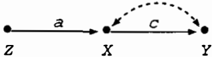
Recently [4], we have shown that the identification of the entire model is ensured if variables standing in di­ rect causal relationship (i.e. , variables connected by arrows in the diagram) do not have correlated errors; no restrictions need to be imposed on errors associated with indirect causes. This class of models was called "bow-free", since their associated causal diagrams are free of any "bow pattern" [10] (see Figure 1).

Most existing conditions for Identification in general models are based on the concept of Instrumental Vari­ ables (IV) [11], [2]. IV methods take advantage of con­ ditional independence relations implied by the model to prove the Identification of specific causal-effects. When the model is not rich in conditional indepen­ dences, these methods are not much informative. In [3], we proposed a new graphical criterion for Identi­ fication which does not make direct use of conditional independence, and thus can be successfully applied to models in which IV methods would fail.

In this paper, we provide an important generalization of the method of Instrumental Variables that makes it less sensitive to the independence relations implied by the model.

2 Linear Models and Identification

An equation Y = (3X + e encodes two distinct as­ sumptions: (1) the possible existence of (direct) causal influence of X on Y; and, (2) the absence of causal in-

fiuence on Y of any variable that does not appear on the right-hand side of the equation. The parameter {3 quantifies the (direct) causal effect of X on Y. That is, the equation claims that a unit increase in X would result in /3 units increase of Y, assuming that every­ thing else remains the same. The variable e is called an "error" or "disturbance"; it represents unobserved background factors that the modeler decides to keep unexplained.

A linear model for a set of random variables Y = {Y1, ... , Yn} is defined formally by a set of equations of the form

and an error variance/covariance matrix I]!, i.e., [IJ!;i] = Cov(e;, ej). The error terms ei are assumed to have normal distribution with zero mean.

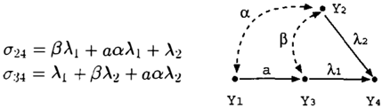
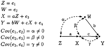
The equations and the pairs of error-terms (e;, ej) with non-zero correlation define the structure of the model. The model structure can be represented by a directed graph, called causal diagram, in which the set of nodes is defined by the variables Y1, ... , Yn, and there is a directed edge from Y; to Yj if the coefficient of Y; in the equation for }j is different from zero. Additionally, if error-terms e; and ei have non-zero correlation, we add a (dashed) bidirected edge between Y; and Y j . Figure 2 shows a model with the respective causal diagram.

The structural parameters of the model, denoted by e, are the coefficients Ci j , and the non-zero entries of the error covariance matrix I]!. In this work, we consider only recursive models, that is, C j i = 0 for i 2: j.

Fixing the model structure and assigning values to the parameters e, the model determines a unique covariance matrix L over the observed variables {Y1, ... ,Yn}, given by (see [1], page 85)

where C is the matrix of coefficients Cji.

Conversely, in the Identification problem, after fixing the structure of the model, one attempts to solve for e in terms of the observed covariance L. This is not always possible. In some cases, no parametrization of the model could be compatible with a given L. In other cases, the structure of the model may permit several distinct solutions for the parameters. In these cases, the model is called nonidentified.

Sometimes, although the model is nonidentifiable, some parameters may be uniquely determined by the given assumptions and data. Whenever this is the case, the specific parameters are identified.

Finally, since the conditions we seek involve the struc­ ture of the model alone, and do not depend on the numerical values of parameters e, we insist only on having identification almost everywhere, allowing few pathological exceptions. The concept of identification almost everywhere is formalized in section 6.

3 Graph Background

Definition 1 A path in a graph is a sequence of edges (directed or bidirected} such that each edge starts in the node ending the preceding edge. A directed path is a path composed only by directed edges, all oriented in the same direction. Node X is a descendent of node Y if there is a directed path from Y to X. Node Z is a collider in a path p if there is a pair of consecutive edges in p such that both edges are oriented toward Z (e.g., ... -t Z +- ... ).

Let p be a path between X and Y, and let Z be an intermediate variable in p. We denote by p[X � Z] the subpath of p consisting of the edges between X and Z.

Definition 2 (d-separation)

A set of nodes Z d-separates X from Y in a graph, if Z blocks every path between X and Y. A path p is blocked by a set Z (possibly empty) if one of the following holds:

• (i) p contains at least one non-collider that is in Z;
• (ii} p contains at least one collider that is outside Z and has no descendant in Z.

4 Instrumental Variable Methods

The traditional definition qualifies a variable Z as in­ strumental, relative to a cause X and effect Y if [10]:

1. Z is independent of all error terms that have an influence on Y which is not mediated by X;
2. Z is not independent of X.

The intuition behind this definition is that all correla­ tion between Z and Y must be intermediated by X.

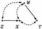
y

Figure 3: Typical Instrumental Variable

\

Y

Figure 4: Conditional IV Examples

If we can find Z with these properties, then the causal effect of X on Y, denoted by c, is identified and given byc=uzyfuzx.

Figure 3 shows a typical example of an instrumental variable. It is easy to verify that variable Z satisfy properties (1) and (2) in this model.

A generalization of the IV method is offered through the use of conditional IV's. A conditional IV is a vari­ able Z that may not have properties (1) and (2), but there is a conditioning set W which makes it happen. When such pair (Z, W) is found, the causal effect of X on Y is identified and given by c = uzY.w / uzx.w.

1. provides the following equivalent graphical crite­ rion for conditional IV's, based on the concept of d­ separation:
2. W contains only non-descendents of Y;
3. W d-separates Z from Y in the subgraph G, ob­ tained by removing edge X -t Y from G;
4. W does not d-separate Z from X in G,.

As an example of the application of this criterion, Figure 4 show the graph obtained by removing edge X -t Y from the model of Figure 2. After condition­ ing on variable W, Z becomes d-separated from Y but not from X. Thus, parameter c is identified.

5 Instrumental Sets

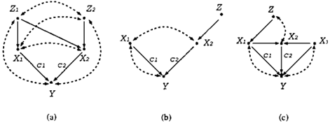
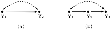
Although very useful, the method of conditional IV's has some limitations. As an example, Figure (5a) shows a simple model in which the method cannot be applied. In this model, variables Z1 and Z2 do not qualify as IV's with respect to either c1 or c2. Also, there is no conditioning set which makes it happen. Therefore, the conditional IV method fails, despite the fact that the model is completely identified.

Following the ideas stated in the graphical criterion for conditional IV's, we show in Figure (5b) the graph

87

obtained by removing edges xl -+ y and x2 -+ y from the model. Note that in this graph, Z1 and Z2 satisfy the graphical conditions for a conditional IV. Intuitively, if we could use both Z1 and Z2 together as instrumental variables, we would be able to identify parameters c1 and c2. This motivates the following informal definition:

A set of variables Z = {Z1, ... , Zk} is called an instrumental set relative to a set of causes X = {X1, ... , Xn} and an effect Y if:

1. Each Z; E Z is independent of all error terms that have an influence on Y which is not mediated by some Xj EX;
2. Each Z; E Z is not independent of the respective X; E X, for appropriate enumerations of Z and X;
3. The set Z is not redundant with respect to Y. That is, for any Z; E Z we cannot explain the correlation between Z; and Y by correlations be­ tween Z; and Z{Z;}, and correlations between Z{Z;} andY.

Properties 1 and 2 above are similar to the ones in the definition of Instrumental Variables, and property 3 is required when using more than one instrument. To see why we need the extra condition, let us consider the model in Figure (5c). In this example, the correlation between Z2 and Y is given by the product of the corre­ lation between z2 and zl and the correlation between Z1 and Y. That is, Z2 does not give additional infor­ mation once we already have Z1. In fact, using Z1 and Z2 as instruments we cannot obtain the identification of the causal effects of X1 and X2 on Y.

Now, we give a precise definition of instrumental sets using graphical conditions. Fix a variable Y and let X = { X1, ... , Xk} be a set of direct causes of Y.

Definition 3 The set Z = {Z1, . · . , Zn} is said to be an Instrumental Set relative to X andY if we can find triples (Z1, W1,p1), . . . , (Zn, Wn,Pn), such that:

• (i) For i = 1, .. . , n, Z; and the elements of W;

are non-descendents of Y; and p; is an unblocked path between Z; and Y including edge X; -+ Y.

• {ii) Let G be the causal graph obtained from G by deleting edges X 1 -+ Y, . . . , X n -+ Y. Then, W; d-separates Z; from Y in G; but W; does not block path p;;
• {iii) For 1 ::; i < j ::; n, variable Zj does not appear in path p;; and, if paths p; and Pj have a common variable V, then both p;[V � Y ] and Pj[Zj � V] point to V.

Next, we state the main result of this paper.

Theorem 1 If Z = { Z 1 , ... , Z n } is an instrumental set relative to causes X = {X1, ... ,X n } and effect Y, then the parameters of edges Xr -+ Y, ... , X n -+ Y are identified almost everywhere, and can be computed by solving a system of linear equations.

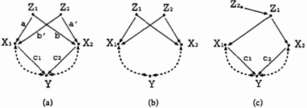
Figure 6 shows more examples in which the method of conditional IV's fails and our new criterion is able to prove the identification of parameters c; 's. In partic­ ular, model (a) is a bow-free model, and thus is com­ pletely identifiable. Model (b) illustrates an interesting case in which variable X2 is used as the instrument for X1 -+ Y, while Z is the instrument for X2 -+ Y. Fi­ nally, in model (c) we have an example in which the parameter of edge X3 -+ Y is nonidentifiable, and still the method can prove the identification of cr and c2.

The remaining of the paper is dedicated to the proof of Theorem 1.

6 Preliminary Results

6.1 Identification Almost Everywhere

Let h denote the total number of parameters in model G. Then, each vector B E Rh defines a parametriza­ tion of the model. For each parametrization B, model G generates a unique covariance matrix I: (B). Let B(A1, ... , A n ) denote the vector of values assigned by B to parameters A1, ... , A n ·

Parameters Ar, ... , A n , are identified almost every­ where if I:(B) = I:(B') implies B(A1, ... , A n ) B' (Ar, ... , A n ) , except when B resides on a set of Lebesgue measure zero.

6.2 Wright's Method of Path Coefficients

Here, we describe an important result introduced by Sewall Wright [12], which is extensively explored in the proof.

Given variables X and Y in a recursive linear model, the correlation coefficient of X and Y, denoted p xv, car, be expressed as a polynomial on the parameters of the model. More precisely,

where term T(pl) represents the multiplication of the parameters of edges along path Pl, and the summation ranges over all unblocked paths between X and Y. For this equality to hold, the variables in the model must be standardized (variance equal to 1) and have zero mean. However, if this is not the case, a simple transformation can put the model in this form [13]. We refer to Eq.(2) as Wright's Equation for X and Y.

Wright's method of path coefficients [12] consists in forming Eq.(2) for each pair of variables in the model, and solving for the parameters in terms of the correla­ tions among the variables. Whenever there is a unique solution for a parameter A, this parameter is identified.

We can use this method to study the identification of the parameters in the model of Figure 5. From the equations for py1 .Ys and py,, y5 we can see that parameters and are identified if and only if

c1 c2 0

6.3 Partial Correlation Lemma

Next lemma provides a convenient expression for the partial correlation coefficient of Y1 and Y2, given Y3, ... , Y n , denoted Pr2.3 . . . n · The proof of the lemma is given in the appendix.

Lemma 1 The partial correlation p12.3 .. n can be ex­ pressed as the ratio:

where ¢> and 'ljJ are functions of the correlations among Y1, Y2, ... , Y n , satisfying the following conditions:

• {ii) ¢(1, 2, ... , n ) is lin ear on the correlations P12, P32, ... , Pnz, with no constant term.
• {iii) The coefficien ts of P1z,p32, ... ,pnz, i n ¢(1, 2, . . . , n ) are polynomials on the corre­ lations among the variables Y1, Y3, . .. , Yn. Moreover, the coefficient of p1z has the con­ stant term equal to 1, and the coefficients of P32, ... , Pnz, are lin ear on the correlations P13, P 1 4, ... , Pin, with no constant term.
• {iv) ('1j;(i1, ... , in-1)) 2 , is a polyn omial on the correlations among the variables Y;,, ... , Y;,_1, with constant term equal to 1.

6.4 Path Lemmas

The following lemmas explore some consequences of the conditions in the definition of Instrumental Sets.

Lemma 2 W.l.o.g., we may assume that, for 1:::; i < j :::; n , paths Pi and PJ do not have any common vari­ able other than (possibly) Zi.

Proof: Assume that paths p; and PJ have some vari­ ables in common, different from Z;. Let V be the closest variable to X; in path Pi which also belongs to path PJ ·

We show that after replacing triple (Z;, W;,p;) by triple (V, Wi,Pi[V � Y]), conditions (i) - (iii) still hold.

It follows from condition (iii) that subpath Pi[V � Y] must point to V. Since p; is unblocked, subpath pi[Z; � V] must be a directed path from V to Z;.

Now, variable V cannot be a descendent of Y, because Pi[Z; � V] is a directed path from V to Z;, and Z; is a non-descendent of Y. Thus, condition ( i) still holds.

Consider the causal graph G. Assume that there exists a path p between V and Y witnessing that Wi does not d-separate V from Y in G. Since p;[Z; � V] is a directed path from V to Z;, we can always find another path witnessing that W; does not d-separate Z; from Y in G (for example, if p and p;[Z; � V] do not have any variable in common other than V, then we can just take their concatenation). But this is a contradiction, and thus it is easy to see that condition ( ii) still holds.

Condition (iii) follows from the fact that p;[V � Y] and PJ[ZJ � V] point to V. 0

In the following, we assume that the conditions of lemma 2 hold.

Lemma 3 For all 1 :::; i :::; n , there exists n o u n blocked path between Z; and Y, different from Pi, which in­ cludes edge X; --+ Y and is composed only by edges from P i , . . . ,p;.

Proof: Let p be an unblocked path between Z; and Y, different from p;, and assume that pis composed only by edges from Pi, ... , Pi·

According to condition (iii), if Z; appears in some path PJ, with j f. i, then it must be that j > i. Thus, p must start with some edges of p;.

Since p is different from Pi, it must contain at least one edge from Pi, . . . , Pi - 1· Let (V1, Vz) denote the first edge in p which does not belong to p;.

From lemma 2, it follows that variable V1 must be a Zk for some k < i, and by condition (iii), both subpath p[Zi � V1] and edge (V1 , Vz) must point to V1. But this implies that p is blocked by vi, which contradicts our assumptions. 0

The proofs for the next two lemmas are very similar to the previous one, and so are omitted.

Lemma 4 For all 1 ::::: i ::::: n, there is no unblocked path between Zi and some Wi; composed only by edges from Pi, ... , p;.

Lemma 5 For all 1 ::::: i ::::: n, there is no unblocked path between Z; and Y i n cluding edge Xj --+ Y, with j < i, composed only by edges from Pi, . . . , p;.

7 Proof of Theorem 1

7.1 Notation

Fix a variable Y in the model. Let X= {X1, .. . , Xk} be the set of all non-descendents of Y which are con­ nected to Y by an edge (directed, bidirected, or both). Define the following set of edges with an arrowhead at Y:

Note that for some X; E X there may be more than one edge between X; and Y (one directed and one bidirected). Thus, l l n c ( Y ) I 2: lXI. Let.\!,··· ,.\m, rn 2: k, denote the parameters of the edges in Inc(Y).

It follows that edges X1 --+ Y, . . . , Xn --+ Y, be­ long to Inc(Y), because X1, . .. , Xn, are clearly non­ descendents of Y. W .l.o.g., let .\; be the parameter of edge X; --+ Y, 1 ::::: i ::::: n , and let .\n+i, .. . , .\m be the parameters of the remaining edges in I n c ( Y ) .

Let Z be any non-descendent of Y. Wright's equation for the pair (Z, Y), is given by

where each term T(p1) corresponds to an unblocked path between Z and Y. Next lemma proves a property of such paths.

Lemma 6 Let Y be a variable in a recursive model, and let Z be a n on-descen dent of Y . Then , any un­ blocked path between Z andY must include exactly one edge from I n c( Y ) .

Lemma 6 allows us to write Eq. (4) as

Thus, the correlation between Z and Y can be expressed as a linear function of the parameters At, ... , Am, with no constant term. Figure 7 shows an example of those equations for a simple model.

7.2 Basic Linear Equations

Consider a triple (Z;, W;,p;), and let W; {W; 1 , · · · , W;.} t . From lemma 1, we can express the partial correlation of Z; and Y given W; as:

where function </>; is linear on the correlations pz,y, Pw,, y, ... , pw,. y, and '1/J; is a function of the corre­ lations among the variables given as arguments. We abbreviate </>;(Z;, Y, W;,, ... , W; ·. ) by </>;(Z;, Y, W;), and '1/J;(V, W;,, ... , W;.) by '1/J;(V, ' W;).

We have seen that the correlations pz, y, pw,, y, ... , Pw,. y, can be expressed as linear functions of the pa­ rameters At, ... , Am. Since </>; is linear on these cor­ relations, it follows that we can express </>; as a linear function of the parameters At, ... , Am.

Formally, by lemma 1, </>;(Z;, Y, W;) can be written as:

Also, for each Vj E {Zi} U W;, we can write:

-----

1To simplify the notation, we assume that IWd = k, for i = 1, . . . , n

Replacing each correlation in Eq.(7) by the expression given by Eq. (8), we obtain

where the coefficients qil 's are given by:

Lemma 7 The coefficients qi,n+I, ... , q;m i n Eq. (9) are identically zero.

Proof: The fact that W; d-separates Z; from Y in G, implies that pz,y.w, = 0 in any probability dis­ tribution compatible with G ([10], pg. 142). Thus, </>;(Z;, Y, W;) must vanish when evaluated in G. But this implies that the coefficient of each of the A; 's in Eq. (9) must be identically zero.

Now, we show that the only difference between evalu­ ations of </>;(Z;, Y, W;) on the causal graphs G and G, consists on the coefficients of parameters AI, ... , An.

First, observe that coefficients b;0, · · · , b;. are poly­ nomials on the correlations among the variables Z;, W;1, · · · , W; ·. Thus, they only depend on the un­ blocked paths between such variables in the causal graph. However, the insertion of edges XI -+ Y, ... , Xn -+ Y, in G does not create any new unblocked path between any pair of Z;, W;1, · · · , W;. (and obvi­ ously does not eliminate any existing one). Hence, the coefficients b;0, · · · , b;· have exactly the same value in the evaluations of </>;(Z;, Y, W;) on G and G.

Now, let At be such that l > n, and let Vj E {Z;} U W;. Note that the insertion of edges XI -+ Y, ... , Xn-+ Y, in G does not create any new unblocked path between Vj and Y including the edge whose parameter is At (and does not eliminate any existing one). Hence, coefficients a;;1, j = 0, ... , k, have exactly the same value on G and G.

From the two previous facts, we conclude that, for l > n, the coefficient of At in the evaluations of </>;(Z;, Y, W;) on G and G have exactly the same value, namely zero. Next, we argue that </>;(Z;, Y, W;) does not vanish when evaluated on G.

Finally, let At be such that l ::; n, and let Vj E { Z;} U W;. Note that there is no unblocked path between Vj and Y in G including edge Xt -+ Y, because this edge does not exist in G. Hence, the coefficient of At in the expression for the correlation PV; y on G must be zero.

On the other hand, the coefficient of At in the same ex­ pression on G is not necessarily zero. In fact, it follows from the conditions in the definition of Instrumental sets that, for l = i, the coefficient of A; contains the term T(p;). D

--;

From lemma 7, we get that ¢;(Z;, Y, W;) is a linear function only on the parameters A1, ... , An.

7.3 System of Equations �

Rewriting Eq.(6) for each triple (Z;, W;,p;), we ob­ tain the following system of linear equations on the parameters A1, ... , An :

where the terms on the right-hand side can be computed from the correlations among the variables Y, Z;, W;1, · · · , W;., estimated from data.

Our goal is to show that � can be solved uniquely for the A; 's, and so prove the identification of A1, ... , An. Next lemma proves an important result in this direc­ tion. Let Q denote the matrix of coefficients of �.

Lemma 8 Det(Q) is a non-trivial polynomial on the parameters of the model.

Proof: From Eq.(lO), we get that each entry q;1 of Q is given by

where b;; is the coefficient of pw, ; y (or pz,y, if j = 0), in the linear expression for ¢;(Z;, Y, W;) in terms of correlations (see Eq.(7)); and ai;l is the coefficient of AI in the expression for the correlation pw, . y in terms J of the parameters A 1 , ... , Am (see Eq.(8)).

From property (iii) of lemma 1, we get that b;0 has constant term equal to 1. Thus, we can write b;0 = 1 + b;0, where b;0 represent the remaining terms of b;0·

Also, from condition ( i) of Theorem 1, it follows that a;0; contains term T(p;). Thus, we can write a;0; = T(p;) + ii;0;, where ii;0; represents all the remaining terms of a;0;.

Hence, a diagonal entry q;; of Q, can be written as

Now, the determinant of Q is defined as the weighted sum, for all permutations 1r of (1, ... , n), of the prod­ uct of the entries selected by 1r (entry qa is selected by permutation 1r if the i1h element of 1r is l), where the weights are 1 or ( -1), depending on the parity of the permutation. Then, it is easy to see that the term

appears in the product of permutation 1r = (1, ... , n), which selects all the diagonal entries of Q.

We prove that det( Q) does not vanish by showing that T' appears only once in the product of permutation (1, ... , n), and that T' does not appear in the product of any other permutation.

Before proving those facts, note that, from the condi­ tions of lemma 2, for 1 :S i < j :S n, paths p; and P i have no edge in common. Thus, every factor ofT' is distinct from each other.

Proposition: Term T' appears only once in the prod­ uct of permutation (1, ... , n ) .

Proof: Let T be a term in the product of permutation (1, ... , n ) . Then, T has one factor corresponding to each diagonal entry of Q.

A diagonal entry q;; of Q can be expressed as a sum of three terms (see Eq.(ll)).

Let i be such that for all l > i, the factor of T corre­ sponding to entry qu comes from the first term of qu (i. e., T(pl)[1 + b10]).

Assume that the factor of T corresponding to entry q;; comes from the second term of q;; (i. e., ii;0;·b;0 ) . Recall that each term in ii;0; corresponds to an unblocked path between Z; and Y , different from p;, including edge X; -+ Y. However, from lemma 3, any such path must include either an edge which does not belong to any of p1, ... ,pn, or an edge which appears in some of Pi+I, ... , Pn · In the first case, it is easy to see that T must have a factor which does not appear in T'. In the second, the parameter of an edge of some PI, l > i, must appear twice as a factor ofT, while it appears only once in T'. Hence, T and T' are distinct terms.

Now, assume that the fa � tor ofT corres � ondin � to en­ try q;; comes from the third term of q;; (1 . e . , Lj =l b;; · a; ; ) . Recall that b;. is the coefficient of Pw y in the J J 1 j expression for ¢;(Z;, Y, W;). From property (iii) of lemma 1, b;; is a linear function on the correlations pz,w, , , . .. , pz,w, . , with no constant term. Moreover, correlation p z , w, , can be expressed as a sum of terms corresponding to unblocked paths between Z; and W;,. Thus, every term in b;; has the term of an unblocked path between Z ; and some W;, as a factor. By lemma 4, we get that any such path must include either an edge that does not belong to any of p1, ... , P n , or an edge which appears in some of Pi+ I, ... , P n · As above,

in both cases T and T* must be distinct terms.

After eliminating all those terms from consideration, the remaining terms in the product of (1, . . . , n ) are given by the expression:

Since b;0 is a polynomial on the correlations among variables W;, , . . . , W;., with no constant term, it fol­ lows that T* appears only once in this expression. 0

Proposition: Term T* does not appear in the prod­ uct of any permutation other than (1, . . . , n ) .

Proof: Let 1r be a permutation different from (1, . . . , n ) , and letT be a term in the product of 1r.

Let i be such that, for all l > i, 1r selects the diagonal entry in the row l of Q. As before, for l > i, if the factor of T corresponding to entry qu does not come from the first term of qu (i.e., T(p1)[1 + b1,]), then T must be different from T*. So, we assume that this is the case.

Assume that 1r does not select the diagonal entry q;; of Q. Then, 1r must select some entry qu, with l < i. Entry qu can be written as:

Assume that the factor of r corresponding to entry qu comes from term b;0 · ai,l· Recall that each term in a;01 corresponds to an unblocked path between Z; and Y including edge X1 -t Y. Thus, in this case, lemma 5 implies that T and T* are distinct terms.

Now, assume that the factor ofT corresponding to en­ try qu comes from term I:�=l b ;, ai ; l· Then, by the same argument as in the previous proof, terms T and T* are distinct. 0

Hence, term T* is not cancelled out and the lemma holds. 0

7.4 Identification of A1, ... , An

Lemma 8 gives that det( Q) is a non-trivial polynomial on the parameters of the model. Thus, det(Q) only vanishes on the roots of this polynomial. However, [8] has shown that the set of roots of a polynomial has Lebesgue measure zero. Thus, system <I> has unique solution almost everywhere.

It just remains to show that we can estimate the entries of the matrix of coefficients of system <I> from data.

Let us examine again an entry qil of matrix Q:

From condition (iii) of lemma 1, the factors b; , in the expression above are polynomials on the correlations among the variables Z;, W;,, . . . , W;., and thus can be estimated from data.

Now, recall that a;01 is given by the sum of terms cor­ responding to each unblocked path between Z; and Y including edge X1 -t Y. Precisely, for each term t in a;, I, there is an unblocked path p between Z; and Y including edge X1 -t Y, such that t is the product of the parameters of the edges along p, except for AI ·

However, notice that for each unblocked path between Z; and Y including edge X1 -t Y, we can obtain an unblocked path between Z; and X1, by removing edge X1 -t Y. On the other hand, for each unblocked path between Z; and X1 we can obtain an unblocked path between Z; andY, by extending it with edge X1 -t Y.

Thus, factor a;,1 is nothing else but pz,x,. It is easy to see that the same argument holds for a; , 1 with j > 0. Thus, a;, I = pw, , x,, j = 0, ... , k.

Hence, each entry of matrix Q can be estimated from data, and we can solve the system of equations <I> to obtain the parameters A1, ... , An.

8 Conclusion

In this paper, we presented a generalization of the method of Instrumental Variables. The main advan­ tage of our method over traditional IV approaches, is that it is less sensitive to the set of conditional indepen­ dences implied by the model. The method, however, does not solve the Identification problem. But, it il­ lustrates a new approach to the problem which seems promising.

Appendix

Proof of Lemma 1: Functions ¢(1, .. . , n ) and 7j;(i1, . .. , i n -d are defined recursively. For n = 3,

-;

For n > 3, we have

Using induction and the recursive definition of P12.3 ... n , it is easy to check that:

Now, we prove that functions q, n and 1/J n 1 as defined satisfy the properties ( i) ( iv). This is clearly the case for n = 3. Now, assume that the properties are satisfied for all n < N.

Property ( i) follows q,N (1, ... , N) and the for q,N - 1 ( 1 , ... ,N -1). from the definition of assumption that it holds

Now, q, N - 1 ( 1 , ... ,N 1) is linear on the correla­ tions P12, ... ,PN - 1,2· Since q,N1 ( 2, N ,3 , ... ,N -1) is equal to q,N - 1 ( N, 2, 3, . . . , N -1), it is linear on the correlations P32, ... , PN,2· Thus, q,N (1, ... , N) is linear on P12, P32, ... , PN ,2, with no constant term, and property ( ii) holds.

Terms ( 'I/J N -2 ( N ,3, ... ,N -1)) 2 and ,p N - 1 ( 1 , N ,3, ... ,N1) are polynomials on the correlations among the variables 1, 3, ... , N. Thus, the first part of property (iii) holds. For the second part, note that correlation p12 only appears in the first term of q,N (1, ... , N), and by the inductive hypothesis ('I/J N-2(N, 3, ... , N1)) 4 has constant term equal to 1. Also, since </J N (1, 2, 3, ... , N) = ,pN (2, 1, 3, ... , N) and the later one is linear on the correlations P12, PI3, ... , PIN, we must have that the coefficients of q,N ( 1, 2, ... , N) must be linear on these correlations. Hence, property (iv) holds.

Finally, for property (iv), we note that by the inductive hypothesis, the first term of ( ¢ N - 2 (N, 3, ... , N -1) ) 2 has constant term equal to 1, and the second term has no constant term. Thus, property (iv) holds. D

References

• [1) K.A. Bollen. Structural Equations with Latent Variables. John Wiley, New York, 1989.
• [ 2 ) R.J. Bowden and D. A. Turkington. Instrumental Variables. Cambridge Univ. Press, 1984.
• [3) C. Brito and J. Pearl. A graphical criterion for the identification of causal effects in linear models. In Proc. of the AAAI Conference, Edmonton, 2002.
• [4) C. Brito and J. Pearl. A new identification con­ dition for recursive models with correlated errors. To appear in Structural Equation Modelling, 2002.
• [5) O.D. Duncan. Introduction to Structural Equation Models. Academic Press, 1975.
• [6) F.M. Fisher. The Identification Problem in Econometrics. McGraw-Hill, 1966.
• [7) R. McDonald. Haldane's lungs: A case study in path analysis. Mult. Beh. Res. , pages 1-38, 1997.
• [8) M. Okamoto. Distinctness of the eigenvalues of a quadratic form in a multivariate sample. Annals of Stat. , 1(4):763-765, July 1973.
• [9) J. Pearl. Causal diagrams for empirical research. Biometrika, 82(4):669-710, Dec 1995.
• [10) J. Pearl. Causality: Models, Reasoning, and In­ ference. Cambridge Press, New York, 2000.
• [11) J. Pearl. Parameter identification: A new per­ spective. Technical Report R-276, UCLA, 2000.
• [12) S. Wright. The method of path coefficients. Ann. Math. Statist., 5:161-215, 1934.
• [1 3 ) S. Wright. Path coefficients and path regressions: alternative or complementary concepts? Biomet­ rics, pages 189-202, June 1960.