Abstract

The paper proposes a numerically stable recursive algorithm for the exact computation of the linear-chain conditional random field gradient. It operates as a forward algorithm over the log-domain expectation semiring and has the purpose of enhancing memory e ffi ciency when applied to long observation sequences. Unlike the traditional algorithm based on the forward-backward recursions, the memory complexity of our algorithm does not depend on the sequence length. The experiments on real data show that it can be useful for the problems which deal with long sequences.

Keywords: conditional random fields, expectation semiring, forward-backward algorithm, gradient computation, graphical models, message passing, sum-product algorithm

1. Introduction

Conditional random fields ( CRF s) [17] are probabilistic discriminative classifiers which can be applied for labeling and segmenting sequential data. When compared with more traditional sequence labeling tools like hidden Markov models ( HMM s), the CRF s o ff er the advantage by relaxing the strong independence assumptions required by HMM s. Additionally, CRF s avoid the label bias problem [17] exhibited by the maximum entropy Markov models and other conditional Markov models based on directed graphical models. However, these improvements are accompanied by a significant cost in time and space needed for the parameter estimation of CRF , especially for real-time problems like labeling very long sequences which appear in computer security [18], [28], bioinformatics [16], [19] and robot navigation systems [15].

The CRF parameter estimation is typically performed by some of the gradient methods, such as iterative scaling, conjugate gradient, or limited memory quasi-Newton methods [12], [17], [21], [23], [25]. All these methods require the computation of the likelihood gradient, which becomes computationally demanding as the sequence length and the number of classes increase. The standard method for gradient computation [17] is based on the internal computation of CRF marginal probabilities by use of the forward-backward ( FB ) algorithm.

The FB algorithm first appeared in two independent publications [4], [5], but it is better known from the subsequent papers

✩ Research supported by Ministry of Science and Technological Development, Republic of Serbia, Grants No. 174013 and 174026

∗ Corresponding author. Tel.: + 381112630170; fax: + 381112186105. Email addresses: [email protected] (Velimir M. Ili´ c), [email protected] (Dejan I. Manˇ cev), [email protected] (Branimir T. Todorovi´ c), [email protected] (Miomir S. Stankovi´ c)

[2], [3]. It makes use of dynamic programming, running with the asymptotical time complexity O( N 2 T ) and with the memory complexity O( NT ) , where T denotes the sequence length and N denotes the number of states classified. In spite of the time e ffi ciency, it becomes spatially demanding when the sequence length is exceptionally large [14]. Furthermore, when it is used for the linear-chain gradient computation as in [12], [17], [21], [23], [25] it requires the storage of all CRF transition matrices which increase the total memory complexity for O( N 2 T ) .

The memory complexity can be reduced with modifications of the FB algorithm such as the checkpointing algorithm [11], [24] or with the re-computation of the transition matrices every time they are used (see section 3.3.). However, these techniques increase the computational complexity, while the memory complexity still depends on the sequence length. Another possibility is the use of forward-only algorithm [6], [20], [22], for which the matrices can be computed in runtime. This algorithm runs with constant memory complexity but it is computationally ine ffi cient since it runs with the computational complexity O( N 4 T ) .

In this paper we propose an algorithm for the exact computation of the linear-chain conditional random field gradient. The algorithm is derived as a forward algorithm over the introduced log-domain expectation semiring, which means that its recursive equations can be obtained if real sums and products from an ordinary FB are replaced with products and sums from the log-expectation semiring. Accordingly, it can be seen as a numerically stable version of our previously developed Entropy Message Passing algorithm (EMP) [13], and it will also be called the EMP. Unlike the standard procedure, the EMP does not compute each marginal separately, but computes the gradient in a single forward pass by use of double recursion.

Gradient Computation In Linear-Chain Conditional Random Fields Using The Entropy Message Passing Algorithm

Velimir M. Ili´ c a,b, ∗ , Dejan I. Manˇ cev b , Branimir T. Todorovi´ c b , Miomir S. Stankovi´ c c

a

Mathematical Institute of the Serbian Academy of Sciences and Arts, Kneza Mihaila 36, 11000 Beograd, Serbia b University of Niˇ s, Faculty of Sciences and Mathematics, Viˇ segradska 33, 18000 Niˇ s, Serbia c University of Niˇ s, Faculty of Occupational Safety, ˇ Carnojevi´ ca 10a, 18000 Niˇ s, Serbia

Since only the forward pass is needed, the EMP can be implemented with the memory complexity being independent of the sequence length, having the advantage over the FB when long sequences are used.

The paper is organized as follows: In section II we explain the FB algorithm which operates over a commutative semiring. In section III we introduce the problem of e ffi cient computation of a linear-chain CRF gradient and review the standard method based on the FB algorithm. The algorithms based on the EMP are presented in section IV, where the complexity analysis is given. Finally, the experimental results are presented in section V where two methods are compared and the advantage of the EMP is discussed.

2. The forward-backward algorithm over a commutative semiring

Definition 1. A commutative semiring is a tuple ( K , ⊕ , ⊗ , 0 , 1 ) where K is the set with operations ⊕ and ⊗ such that both ⊕ and ⊗ are commutative and associative and have identity elements in K ( 0 and 1 respectively), and ⊗ is distributive over ⊕ .

Let ( K , ⊕ , ⊗ , 0 , 1 ) be a commutative semiring and let y = { y 0 , . . . , yT } be a set of variables taking values from the set Y of cardinality N . We define the local kernel functions ut ∶ Y 2 → K for t = 1 , . . . , T , and the global kernel function u ∶ Y T + 1 → K , assuming that the following factorization holds

for all y = ( y 0 , . . . , yT ) ∈ Y T + 1 .

The FB algorithm [26], [27] solves two problems

1. The marginalization problem: Computes the sum

2. The normalization problem: Computes the sum

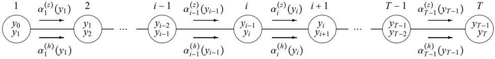
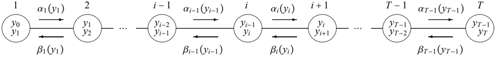
The FB recursively computes the forward vector

which is initialized to

and recursively computed using

and the backward vector

which is recursively computed using

and initialized to

Once the forward α k -1 and backward β k vectors are computed, we can solve the marginalization problem by use of the formula

The normalization problem can be solved with the forward pass only according to

3. Linear-Chain CRF Training using the Forward Backward Algorithm

Linear-chain CRFs are discriminative probabilistic models over observation sequences x = ( x 1 , . . . , xT ) and label sequences y = ( y 1 , . . . , yT ) , defined with conditional probability

The symbol ⟨ ⋅ , ⋅ ⟩ denotes the scalar product between an M -dimensional parameter vector

and the feature vector on position i

The normalization factor

is called the partition function .

The goal of the CRF training is to build up the model (12) from the data set {( x ( d ) , y ( d ) } D d = 1 . The standard method is to maximize the log likelihood of (12):

over the parameter vector θ for the chosen set of feature vectors f ( yi -1 , yi , x , i ) . The maximum can be found with several of the gradient methods [12], [17], [21], [23], [25], which requires the computation of the gradient ∇ θ L ( θ ) . The gradient can be expressed, according to (12) and (16), as:

as

where T ( d ) is the length of the d -th observation sequence.

The main problem in the evaluation of the log likelihood gradient (17) is the computation of the quotient between the partition function gradient and the partition function. The partition function gradient can be represented as

where ∇ θ m Z ( x ; θ ) denotes the m -th partial derivative, and can be obtained from (15) after the use of the Leibniz's product rule:

The standard method for the computation of the partition function and its gradient [17] is based on the forward-backward algorithm which is reviewed in the following section.

3.1. Sum-product semiring forward-backward algorithm

Definition 2. The sum-product semiring is the tuple ( R , +⋅ , 1 , 0 ) , where R is the set of real numbers and the operations defined in a standard way.

The partition function (15) can be obtained as the solution of the normalization problem (11) for factorization:

The gradient can be computed using the solution for the marginalization problem (10) in the sum-product semiring. First, we change the sum ordering in (19) and split the sum over y to y { k -1 , k } and y { k -1 , k } c sums, transforming (19) to:

The marginal values,

as the marginalization problem over the sum-product semiring, can be found by recursive computation of forward vectors,

and backward vectors

The FB algorithm over the sum-product semiring su ff ers from numerical instability since the exponential terms can fall out of the machine precision scope and it is usually replaced with a more stable FB algorithm over the log-domain sumproduct semiring.

3.2. Log-domain sum-product semiring forward-backward algorithm

Definition 3. The log-domain sum-product semiring is the tuple ( R ∗ , ⊕ , ⊗ , -∞ , 0 ) where R ∗ is the extended set of real numbers and the operations are defined by

for all a , b ∈ R .

The following lemma follows straightforwardly from the definition of the log-domain sum-product semiring.

Lemma 1. Let ai ∈ R for all 1 ≤ i ≤ T. Then, the following equalities hold for log-domain sum-product semiring:

In log-domain the local kernels have the form:

for i = 1 , . . . , T . According to Lemma 1 and expression (4), the forward vector in the log-domain sum-product semiring is the logarithm of the forward vector in the sum-product semiring:

The forward vector α 0 is initialized to 0 which is the identity for ⊗ ,

and it is recursively computed using

Similarly to Lemma 1 and to expression (7), the backward vector in the log-domain sum-product semiring is the logarithm of the backward vector in sum-product semiring:

being initialized to and recursively computed using

If the log-domain addition is performed using the definition, a ⊕ b = ln ( e a + e b ) , the numerical precision is being lost when computing e a and e b . But, as noted in ([23]), ⊕ can be computed as

which can be much more numerically stable, particularly if we pick the version of the identity with the smaller exponent.

The logarithm of the normalization constant (21) is according to Lemma 1

and it can be computed using the solution of normalization problem in the log-domain sum-product semiring with forward algorithm according to (11)

According to Lemma 1, the marginal values (23) in the logdomain sum-product semiring have the form

The marginal values can e ffi ciently be computed according to the solution of the marginalization problems (10):

where α k -1 ( yk -1 ) and β k ( yk ) are computed with the FB algorithm over the log-domain sum-product semiring, using equations (31)-(35). Then, by taking the logarithm of the m -th component in gradient expression (22), we get

for m = 1 , . . . , M . Finally, the quotient between the partition function and its gradient can be computed according to

Algorithm 1: Log-domain FB algorithm

3.3. Time and Memory Complexity

The time and memory complexity of the algorithm for the computation of the partition function and its derivatives by the FB algorithm is given in Table 1. The time complexity is defined as the number of operations required for the execution of the algorithm for a given pseudo code. In our analysis we consider real operations (addition and multiplication), log-domain

Table 1: Time and memory complexity of the log-domain FB algorithm.

	⊕	+	×	ln	Mem
u α β	- N 2 T 2	N 2 TA N 2 T N 2 T 2 N 2 T - - N 2 TA 2	N 2 TA	- -	N 2 T NT NT 1 1
			-
	N T		-	-
v	-		-	-
ln f	-		-	N 2 TA
ln Z ( x ; θ )	N		-	-	1
ln ∇ θ m Z ( x ; θ )	N 2 TA		-	-	M
Asymptotical	N 2 TA	2 N TA	N 2 TA	N 2 TA	N 2 T + M

operations (recall that log-domain multiplication is defined as real addition) and the number of computed logarithms. The memory complexity is defined as the number of 32-bit registers needed to store variables during algorithm execution. The complexity expressions are simplified by taking the quantities in expressions to tend to infinity, and keeping only the leading terms. In discussion, we will use big O notation [7].

In applications, the feature functions f ( yk -1 , yk , x , k ) map the input space for a fixed sequence x into sparse vectors, which has nonzero values only at positions

which allows the complexity reduction by performing the computation only for nonzero elements. In our analysis we will use the average number of nonzero elements defined as

As Table 1 shows, the computationally most demanding part of the algorithm is the termination phase, which requires O( N 2 TA ) log-additions (recall that one log-addition requires the computation of the exponent and logarithm). The memory complexity of the algorithm is O( N 2 T + M ) , governed by the space needed for storing the matrices ui . The dependence of the memory complexity on the sequence length can significantly decrease computational performances of the algorithm if a long sequence is used, since it can cause overflows from the internal system memory to the disk storage, as shown in section 5.

The memory complexity can be reduced by the recomputation of the matrices ui in the backward pass (line 14) and in the termination step (line 19), but this leads to the increased total number of additions and multiplications for 2 N 2 TA , while the memory complexity still depends on the sequence length since all forward and backward vectors need to be stored. The further improvement can be achieved if one notes that the backward vectors are computed during the termination step since they are used only once in line 19. In this case, each backward vector can be deleted after use in line 19 and all backward vectors can be stored at the memory location not depending on the sequence length. Then, the matrices ui can be recomputed only once in the termination step, where they are used for the computation of the backward vector but, again, all forward vectors need to be stored and the memory complexity is O( NT + M ) , still depending on the sequence length.

The checkpointing algorithm [11], [24] divides the input sequence into √ T and during the forward pass only stores the first forward vector in each sub-sequence (checkpoint vectors). In the backward pass, the forward values for each sub-sequence are sequentially recomputed, beginning with checkpoint vectors. In this way, the computational complexity required for the computation of the forward and backward vectors is increased to O( 2 T -N 2 √ T ) , while the matrices ui should also be recomputed, which leads to greater total computational cost. On the other hand, the memory complexity, although reduced to O( N √ T ) , still depends on the sequence length.

The problem of memory complexity of the forwardbackward algorithm for the HMM has already been studied by Khreich et al. in [14]. In this paper they have proposed the algorithm for the computation of marginal probabilities called forward filtering backward smoothing ( EFFBS ), which runs with the memory complexity independent of the sequence length, O( N ) , with the same asymptotical computational complexity as the standard forward-backward algorithm. However, the algorithm is based on the HMM assumption that the transition matrix is constant, and as such cannot be applied to CRF s. Khreich et al. also gave a good review of the previously developed techniques for memory reduction such as checkpointing and forward-only algorithm, which try to reduce the memory complexity of the FB algorithm at the cost of computational overhead, and these techniques can be modified to deal with CRF s.

In the forward-only algorithm [6], [14], [20], [22], the expression of the form is obtained from three-dimensional matrices which are recursively computed. For the HMM , the computation can be realized in the constant memory space independent of the sequence length O( N 2 + N ) and with time complexity O( N 4 T ) . However, if it is applied to the CRF , its time complexity increases to O( N 4 MT ) , which is significantly slower than the FB algorithm.

In the following section we derive a forward-only algorithm which operates with the time complexity of order O( N 2 ( M + A ) T ) , while keeping the memory complexity independent of

the sequence length.

4. Log-domain expectation semiring forward algorithm

In this section we consider a memory-e ffi cient algorithm for CRF gradient computation which operates as a FB algorithm over an expectation semiring and develop its numerically stable log-domain version. In our previous work [13], we have developed the Entropy Message Passing EMP , which operates as a forward algorithm over the entropy semiring, which is the special case the expectation semiring. Although the algorithms presented in this paper are more general, in the following text they will be called the EMP , since they operate in the same manner as the algorithm from [13].

4.1. Expectation semiring forward algorithm

Definition 4. The expectation semiring of an order M is a tuple ⟨ R × R M , ⦶ , ⊙ , ( 0 , 0 ) , ( 1 , 0 ) ⟩ , where the operations ⦶ and ⊙ are defined with:

for all ( z 1 , h 1 ) , ( z 2 , h 2 ) from R × R M , and 0 denotes zero vector. The first component of an ordered pair is called a z-part, while the second one is an h-part.

For M = 1, the expectation semiring reduces to the entropy semiring considered in [13]. According to the addition rule, the z and h components of sum of two pairs are the sums of z and h components respectively, which gives us the following lemma.

Lemma 2. Let ( zi , h i ) ∈ R × R M for all 1 ≤ i ≤ T. Then, the following equality holds in the expectation semiring:

Note that if the pairs have the form ( z , z h ) , the multiplication acts as

This can be generalized with the following lemma.

Lemma 3. Let ( zi , zi h i ) ∈ R × R M for all 1 ≤ i ≤ T. Then, the following equality holds in the expectation semiring:

According to lemma 3, if the local kernels have the form:

for i = 1 , /uni22EF , T , the global kernel is, according to the Lemma 3

By applying lemma 2 to the expression (51), we can obtain the partition function (15),

and its gradient (19):

as z and h parts of the sum

The expression (54) can be computed as the normalization problem (11) by use of the forward algorithm over the expectation semiring. Note that z -parts of addition and multiplication acts as addition and multiplication in the sum-product semiring. Accordingly, the z -parts of forward vectors will be the same as the forward vectors in the sum-product semiring, and their computation is numerically unstable. In the following subsection we a develop numerically stable forward algorithm which operates over a log-domain expectation semiring.

4.2. Log-domain expectation semiring forward algorithm

The log-domain expectation semiring is a combination of the log-domain sum-product semiring and the expectation semiring. It can be obtained if real addition and multiplication in the definition of expectation semiring operations are replaced with their log-domain counterparts.

Before we define the log-domain expectation semiring, we introduce some usefull notation. Firstly, recall that log-domain addition and multiplication are defined with

The log-product between the scalar z ∈ R and the vector h = ( h [ 1 ] , . . . , h [ M ]) ∈ R M is defined as the vector z ⊗ h :

the logarithm of the vector [ h 1 , . . . , hM ] ∈ R M is defined as

The vector -∞ is defined as a vector all of whose coordinates are -∞ .

Definition 5. The log-domain expectation semiring of an order M is a tuple ⟨ R × R M , ⦶ , ⊙ , ( -∞ , -∞ ) , ( 0 , -∞ ) ⟩ , where the operations ⦶ and ⊙ are defined with:

or, using the operations from the log-domain sum-product semiring,

for all ( z 1 , h 1 ) , ( z 2 , h 2 ) from R × R M . Similar to the expectation semiring, the first component of an ordered pair is called a zpart, while the second one is an h-part.

The following lemma is the log-domain version of Lemma 2.

Lemma 4. Let ( zi , zi h i ) ∈ R × R M for all 1 ≤ i ≤ T. Then, the following equality holds in the log-domain expectation semiring:

where

Similar to the expectation semiring, if the pairs have the form ( z , z ⊗ h ) the multiplication acts as

The following lemma is the log-domain version of Lemma 3.

Lemma 5. Let ( zi , zi ⊗ h i ) ∈ R × R M for all 1 ≤ i ≤ T. Then, the following equality holds in the log-domain expectation semiring:

where

Let for i = 1 , . . . , T

Then, the logarithm partition function (15) can be written as

The logarithm of the m -th partial derivative can be written as

If the local kernels have the form:

for i = 1 , /uni22EF , T , the global kernel is, according to Lemma 5

Furthermore, Lemma (4) for addition in the expectation semiring implies that the sum of ordered pairs is the ordered pair of the sums so the partition function and its gradient can be found as the z and h part of the sum:

Expression (72) can be computed as the normalization problem (11) by use of the forward algorithm over the log-domain expectation semiring ( log-domain EMP algorithm ). The forward algorithm is initialized to the log-domain expectation semiring identity for the multiplication:

for all y 0 ∈ Y . After that, we compute other forward vectors using the recurrent formula

where the local factors are given with (70).

According to the rules for the addition and multiplication in the expectation semiring, the z and h parts of recursive equation (74) are:

for each yi ∈ Y , i = 1 , . . . T . Finally, the normalization problem can be solved by summation

whose z part is a partition function and the h part is its gradient:

Hence, the algorithm consists of two parts: i) forward pass , at which the forward vectors are initialized according to (73) and recursively computed by (75)-(76), and during each step the corresponding matrix ui is computed and ii) termination , at which the final summation of the forward algorithm is performed according to (78) and the partition function and its derivatives are obtained.

Figure 2 describes the EMP computation scheme. Recall that the forward-backward based computation requires that all forward and backward vectors be computed and stored until the partition function and the derivatives are obtained in the termination step. When the EMP is used, the computation terminates when the last forward vector is computed by use of the formulas (75) and (76). This can be realized in the fixed memory space with the size independent of the sequence length since the vectors α ( z ) i -1 , α ( h ) i -1 and the matrices ψ i should be computed only once in i -1-th iteration and, after having been used for the computation of α ( z ) i and α ( h ) i , they can be deleted. The pseudo code is given in the table Algorithm 2. Here, the computation is performed using only two pairs of vectors ( ˆ α ( z ) , ˆ α ( h ) ) and ( α ( z ) , α ( h ) ) . Note that the coordinates of the h -parts, ˆ α ( h ) ( yi ) and α ( h ) ( yi ) , are vectors which carry the information about the gradient and the m -th components of these vectors are denoted with ˆ α ( h ) [ m ] ( yi ) and α ( h ) [ m ] ( yi ) .

In comparison to the FB algorithm which needs the memory size of O( N 2 T + M ) , the EMP has a memory complexity O( N 2 + NM ) , no longer depending on the sequence length T as in the FB algorithm. The additional cost is paid in time complexity which is increased for the term N 2 TM . This is the consequence of the non-sparse computation of the EMPh component in line 13. Recall that the FB can be completely sparse implemented and, since A << M in most of the application, the FB time complexity is lower. However, the sparsity can be reduced using the conditionally trained hidden Markov model assumption considered in [29], which we used in our implementation. With the reduced sparsity, the time complexity of the EMP is decreased and it becomes closer to the FB algorithm. When long sequences are used, the EMP becomes dominating since the FB needs to use the external memory. This assertion is justified in the following section, where we compare the two algorithms on a real data example.

5. Experiments

The intrusion detector learning task is to build a predictive model capable of distinguishing between 'bad' connections,

Algorithm 2: Log-domain EMP algorithm

input : x , θ , f ( yj -1 , yj , x , j ) ; j = 1 , . . . , T , yj -1 , yj ∈ Y ; output : ∇ θ Z ( x ; θ )/ Z ( x ; θ ) ; /* Forward algorithm */ 1 foreach y 0 in Y do 2 α ( z ) ( y 0 ) ← 1 3 for m ← 1 to M do 4 α ( h ) [ m ] ( y 0 ) ← -∞ ; 5 for i ← 1 to T do 6 foreach yi in Y do 7 foreach yi -1 in Y do 8 ψ ( yi -1 , yi ) = ⟨ θ , f ( yi -1 , yi , x , i )⟩ ; 9 foreach yi in Y do 10 ˆ α ( z ) ( yi ) = ⊕ yi -1 ( ψ ( yi -1 , yi ) + α ( z ) ( yi -1 )) ; 11 for m ← 1 to M do 12 foreach yi in Y do 13 ˆ α ( h ) [ m ] ( yi ) ← ⊕ yi -1 ( ψ ( yi -1 , yi ) + α ( h ) [ m ] ( yi -1 )) ; 14 foreach yi -1 in Y do 15 foreach yi in Y do 16 γ ( yi -1 ) ← ψ ( yi -1 , yi ) + α ( z ) ( yi -1 ) ; 17 foreach m in A( yi -1 , yi ) do 18 ln f ← ln fm ( yi -1 , yi , x , i ) ˆ α ( h ) [ m ] ( yi ) ← ˆ α ( h ) [ m ] ( yi ) ⊕ ( γ ( yi -1 ) + ln f ) ; 19 foreach yi in Y do 20 α ( z ) ( yi ) ← ˆ α ( z ) ( yi ) ; 21 for m ← 1 to M do 22 α ( h ) [ m ] ( yi ) ← ˆ α ( h ) [ m ] ( yi ) ; /* Termination */ 23 ln Z ← ⊕ yT α ( z ) ( yT ) 24 ln ∇ mZ ← ⊕ yT α ( h ) [ m ] ( yT ) 25 for m ← 1 to M do 26 ∇ θ m Z ( x ; θ )/ Z ( x ; θ ) ← e ln ∇ mZ -ln Z

called intrusions or attacks, and 'good' normal connections. Conditional random fields have proven to be very e ff ective in detecting intrusion [30].

As we have already mentioned, in the standard CRF training based on the FB algorithm the storage requirements are high when long train sequences are used. This may cause overflows from the internal system memory to disk storage which decreases computational performances, since accessing paged memory data on a typical disk drive is significantly slower than accessing data in RAM [14],[28]. On the other hand, the EMP runs with a small fixed memory and it becomes preferable for long sequences.

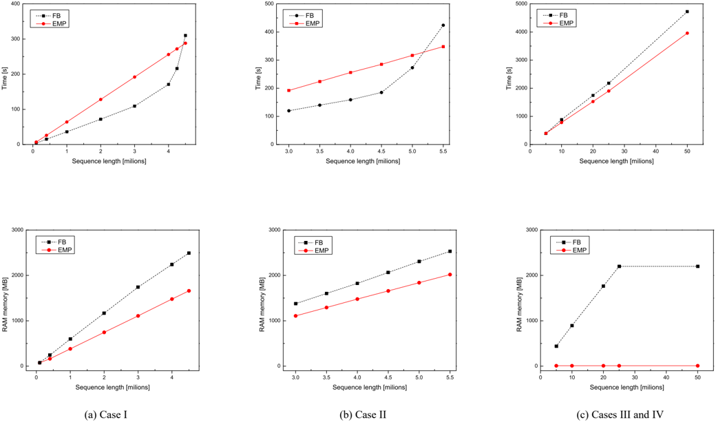
In Figure 3 we show the time and memory usage of both al-

Table 2: Time and memory complexity of the log-domain EMP algorithm.

	⊕	+	×	ln	Mem
ψ ˆ α ( z ) γ ˆ α ( h ) m α ( z ) ln f α ( h ) r Z ( x ; (	- N 2 T - N 2 T -	N 2 TA N 2 T N 2 T N 2 T ( - - - -	N 2 TA - -	-	N 2 N 1 NM N 1
				-
				-
	( M + A )	M + A )	-	N 2 TA
			-	-
	-		-	N 2 TA
	-		-	-	NM
ln θ )	N		-	-	1
ln ∇ θ m Z x ; θ )	NM	-	-	-	M
Asymptotical	N 2 T ( M + A )	N 2 T ( M + 2 A )	N 2 TA	N 2 TA	N 2 + NM

/s32

/s32

/s32

gorithms as functions of the sequence length. The experiments are performed using a computer with 3GB RAM and IntelCore 2 Duo CPU 2.33GHz. In our experiments, we used a KDE corpus [31] for sequences up to 5 million, while the sequences longer than 5 million are created by the concatenation of the KDE corpus on itself. We consider four di ff erent implementation cases depending on the sequence length:

Case I: This corresponds to short sequences, with the length shorter than 4 million. This case corresponds to the basic version of the FB algorithm (Algorithm 1). In this case, the se- quence is stored in RAM and the RAM usage of both algorithms linearly grows with the sequence length (Figure 3a). However, the FB algorithm uses O( N 2 T + M ) memory for storing intermediate results and its RAM usage grows faster in comparison to the EMP , which needs fixed-size additional space O( N 2 + NM ) . RAM usage growth reflects on the computational performances of FB algorithm, which runs faster then the EMP for the sequences with the length up to 4 . 5 million. As Figure 3a shows, at the sequence length of 3 millions FB RAMusage becomes considerable and the FB growth becomes

/s32

nonlinear due to the memory paging. Finally, at the sequence length of about 4 . 5 million the EMP becomes faster than FB . One possibility for FB memory reduction is recomputation of transition matrices which is done in the Case II.

Case II: This corresponds to middle length sequences, between 4 and 5 million. At this case the sequence and all intermediate results are stored in RAM, but the transition matrices are recomputed every time they are used. Similar to the Case I, as the sequence becomes longer, the memory required for storing the forward vectors increases and, for sequences longer then 5 million, FB algorithm becomes slower than the EMP (see Figure 3b).

Case III: This corresponds to long sequences between 5 and 25 million. As in Case II, transition matrices are recomputed and all another intermediate results are stored in RAM, but the sequence cannot fit in RAM and needs to be stored on the secondary memory. In the FB the sequences have to be read twice from secondary memory, once in the forward and once in the backward phase. On the other hand, the EMP uses a single forward pass and reads the sequence only once, which makes it faster than the FB (Figure 3c).

Case IV: This corresponds to very long sequences loger than 25 million. In this case, similar to the Case III , the sequence is stored on the secondary memory. To avoid the FB performance decreasing due to a large number of intermediate variables stored in RAM , the portion of variables is stored on the secondary memory, which keeps the RAM usage constant, no longer dependent on the sequence length (Figure 3c). This increases the number of accessions to the secondary memory, which further decreases FB performances in comparison to Case III . On the other hand, the EMP does not need to store additional data on the secondary memory and has the same time growth as in Case III , while using a small constant memory.

The previous results can vary with di ff erent operating systems and used hardware. Nevertheless, the access to secondary memory is very expensive operation and the algorithm with a low memory complexity has the advantage, when all data cannot fit in RAM, since the secondary memory accesses can be avoided.

6. Conclusion

In this paper, we have developed a numerically stable algorithm for the computation of the linear-chain CRF gradient. As opposed to the standard way of finding a CRF gradient by use of the forward-backward algorithm, the calculation by the proposed algorithm requires only the forward pass and can be realized with the memory independent of the observation sequence length. This makes the algorithm useful in the long sequence labeling tasks found in computer security [18], [28], bioinformatics [16],[19], and robot navigation systems [15].

The proposed algorithm operates as a forward algorithm over the log-domain expectation semiring, which can be seen as a modification of the expectation semiring used in the automata theory and probabilistic context free grammars [32], [33]. As mentioned in the paper, the use of the expectation semiring leads to numerically unstable algorithms and its log-domain counterpart can also be applied to numerically stable solutions of problems considered in [32], [33].

7. References

References

1. S.M. Aji and R.J. McEliece. The generalized distributive law. Information Theory, IEEE Transactions on , vol. 46(2), pages 325 -343, 2000.
2. L. Bahl, J. Cocke, F. Jelinek, and J. Raviv. Optimal decoding of linear codes for minimizing symbol error rate (corresp.). Information Theory, IEEE Transactions on , vol. 20(2), pages 284 - 287, 1974.
3. L. Baum. An inequality and associated maximization technique in statistical estimation for probabilistic functions of Markov processes. Inequalities , vol. 3, pages 1-8, 1972.
4. Leonard E. Baum and Ted Petrie. Statistical inference for probabilistic functions of finite state markov chains. The Annals of Mathematical Statistics , vol. 37(6), pages 1554-1563, 1966.
5. R. Chang and J. Hancock. On receiver structures for channels having memory. Information Theory, IEEE Transactions on , vol. 12(4), pages 463 - 468, 1966.
6. Alexander Churbanov and Stephen Winters-Hilt. Implementing em and viterbi algorithms for hidden markov model in linear memory. BMC Bioinformatics , vol. 9(224), 2008.
7. Thomas H. Cormen, Charles E. Leiserson, Ronald L. Rivest, and Cli ff ord Stein. Introduction to Algorithms . McGraw-Hill Science / Engineering / Math, 2nd edition, 2003.
8. Cortes C., Mohri M., Rastogi A., and Riley M., On the computation of the relative entropy of probabilistic automata, International Journal of Foundations of Computer Science , vol. 19, pages 219-242, 2007.
9. Robert G. Cowell, Philip A. Dawid, Ste ff en L. Lauritzen, and David J. Spiegelhalter. Probabilistic Networks and Expert Systems (Information Science and Statistics) . Springer, New York, 2003.
10. Eisner J., Parameter estimation for probabilistic finite-state transducers. in Proceedings of the 40th Annual Meeting of the Association for Computational Linguistics , pages 1-8, 2002.
11. J. Alicia Grice, Richard Hughey, and Don Speck. Reduced space sequence alignment. Computer Applications in the Biosciences , vol. 13(1), pages 45-53, 1997.
12. Rahul Gupta. Conditional random fields, 2006. Technique Report, IIT Bombay.
13. Velimir M. Ili´ c, Miomir S. Stankovi´ c, and Branimir T. Todorovi´ c. Entropy message passing algorithm. IEEE Transactions on Information Theory , vol 57(1), pages 375-380, 2011.
14. Wael Khreich, Eric Granger, Ali Miri, and Robert Sabourin. On the memory complexity of the forward-backward algorithm. Pattern Recognition Letters , vol 31(2), pages 91-99, 2010.
15. Sven Koenig and Reid G. Simmons. Unsupervised learning of probabilistic models for robot navigation. In in Proceedings of the IEEE International Conference on Robotics and Automation , pages 2301-2308, 1996.
16. Anders Krogh, Michael Brown, I. Saira Mian, Kimmen Sjlander, and David Haussler. Hidden markov models in computational biology: applications to protein modeling. Journal of Molecular Biology , vol. 235, pages 1501-1531, 1994.
17. John La ff erty, Andrew Mccallum, and Fernando Pereira. Conditional random fields: Probabilistic models for segmenting and labeling sequence data. In Proc. 18th International Conf. on Machine Learning , pages 282289, 2001.
18. Terran D. Lane. Machine learning techniques for the computer security domain of anomaly detection, PhD thesis, Purdue University, USA, 2000.
19. Irmtraud M. Meyer and Richard Durbin. Gene structure conservation aids similarity based gene prediction. Nucleic acids research , vol. 32(2), pages 776-783, 2004.
20. I. Mikl´ os and I. M. Meyer. A linear memory algorithm for baum-welch training. BMC bioinformatics , vol. 6, 2005.
21. Fei Sha and Fernando Pereira. Shallow parsing with conditional random fields. In NAACL '03 , vol.1, pages 213-220, 2003.

1. S. Sivaprakasam and K. Sam Shanmugan. A forward-only recursion based hmm for modeling burst errors in digital channels. In GLOBECOM '95 , vol.2, pages 1054 -1058, 1995.
2. Charles A. Sutton. E ffi cient training methods for conditional random fields . PhD thesis, 2008.
3. Christopher Tarnas and Richard Hughey. Reduced space hidden markov model training. BIOINFORMATICS , vol. 14(5), pages 401-406, 1998.
4. S. V. N. Vishwanathan, Nicol N. Schraudolph, Mark W. Schmidt, and Kevin P. Murphy. Accelerated training of conditional random fields with stochastic gradient methods. In ICML , pages 969-976, 2006.
5. F. R. Kschischang, B. J. Frey, and H.-A. Loeliger. Factor graphs and the sum-product algorithm. IEEE Trans. Inform. Theory , vol. 47, pp. 498519, 2001.
6. S. M. Aji and R. J. McEliece. The generalized distributive law. IEEE Trans. Inform. Theory , vol. 46, pp. 325-343, Mar. 2000.
7. C. Warrender, S. Forrest, and B. Pearlmutter. Detecting intrusions using system calls: alternative data models. In IEEE Symposium on Security and Privacy, pages 133 -145, 1999.
8. Shaolei Feng, R. Manmatha, and Andrew McCallum and Kevin P. Exploring the Use of Conditional Random Field Models and HMMs for Historical Handwritten Document Recognition. DIAL '06 , pages 30-37, 2006.
9. Kapil Kumar Gupta, Baikunth Nath, and Kotagiri Ramamohanarao. Conditional Random Fields for Intrusion Detection. In AINAW '07 , vol.1, pages 203-208, 2007.
10. KDE-CUP-99 Task description:

http: // kdd.ics.uci.edu / databases / kddcup99 / task.html

1. J. Eisner, 'Parameter estimation for probabilistic finite-state transducers,' In Proceedings of the 40th Annual Meeting of the Association for Computational Linguistics , Philadelphia, July 2002, pp. 18.
2. Z. Li, J. Eisner. First- and second-order expectation semirings with applications to minimum-risk training on translation forests, In Proceedings of the 2009 Conference on Empirical Methods in Natural Language Processing , Volume 1 - Volume 1, EMNLP '09, pp. 40-51, Morristown, NJ, USA, 2009. Association for Computational Linguistics.