Logarithmic Time Parallel Bayesian Inference

David M. Pennock

University of Michigan AI Laboratory 1101 Beal Avenue Ann Arbor, MI 48109-2110 USA dpennock@ umich.edu

Abstract

I present a parallel algorithm for exact prob­ abilistic inference in Bayesian networks. For polytree networks with n variables, the worst­ case time complexity is O(log n ) on a CREW PRAM (concurrent-read, exclusive-write paral­ lel random-access machine) with n processors, for any constant number of evidence variables. For arbitrary networks, the time complexity is O( r3w log n ) for n processors, or 0( w log n ) for r3w n processors, where r is the maximum range of any variable, and w is the induced width (the maximum clique size), after moralizing and trian­ gulating the network.

1 INTRODUCTION

Two key breakthroughs make representation of and reaso � ­ ing with probabilities practical, and have led to a prolif­ eration of related research within the artificial intelligence community. Bayesian networks exploit conditional inde­ pendence to represent joint probability distributions com­ pactly, and associated inference algorithms evaluate ar­ bitrary conditional probabilities implied by the network representation (Neapolitan 1990; Pearl 1988) : Exact in­ ference is known to be NP-hard (more specifically, #P­ complete) (Cooper 1990), and even approximate inference is NP-hard (Dagum and Luby 1993). Nonetheless, clever algorithms exploit network topology to make exact proba­ bilistic reasoning practical for a wide variety of real-world applications. Although no algorithm, including any par­ allel algorithm with a polynomial number of processors, can avoid worst-case exponential time complexity (unless p = NP), polynomial time speed-ups are still of great in­ terest, to allow evaluation of larger, more densely connected Bayesian networks.

Some researchers have proposed parallel algorithms for Bayesian inference (D'Ambrosio 1992; Diez and Mira

(a)

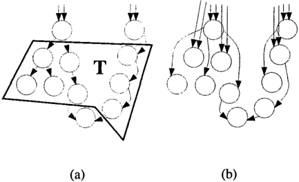
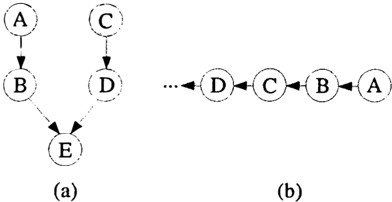
Figure 1: Comparing the Opportunities for Parallelism in Two Bayesian Networks. Network (a) seems to have more "natural" parallelism.

1994; Kozlov 1996; Kozlov and Singh 1994; Shachter, An­ dersen, and Szolovits 1994). In fact, Pearl's original algo­ rithm for inference in singly connected networks was con­ ceived as a distributed algorithm, where each variable could be associated with a separate processor, passing and receiv­ ing messages to and from only local, neighboring proces­ sors (Neapolitan 1990; Pearl 1988). The popular junction tree algorithm for multiply connected networks (Jensen, Lauritzen, and Olesen 1990; Lauritzen and Spiegelhalter 1988; Neapolitan 1990; Spiegelhalter, Dawid, Lauritzen, and Cowell 1993) can be considered a distributed algo­ rithm in the same sense, with one processor per clique. However, to my knowledge, there are no derivations of improved worst-case complexity bounds for parallel in­ ference, mainly because previous attempts at paralleliza­ tion only exploit concurrency in the form of independent computations. For example, consider the two networks in Figure 1. In both (a) and (b), the two computations Pr(B bi) ,_ L: A Pr(B b1JA) Pr(A) and Pr(B = b2) ,_ L: A Pr(B = b2JA) Pr(A) are in­ dependent and easily parallelized. D'Ambrosio (1992) calls this a conformal product parallelization, while Ko­ zlov and Singh (1996, 1994) call it a within-clique par­ allelization. In network (a), the computations Pr( B) <­ I: Pr(BJA) Pr(A) and Pr(D) ,_ l::c Pr(DJC) Pr(C) ar / also independent; this has been called topological par­ allelism. However in the chain network (b), the computa-

tion Pr(D) ,._ Lc Pr(DIC) Pr(C) must wait for the com­ putation of Pr( C), which must in turn wait for the com­ putation of Pr( B), etc. Because of the possibility of such chains, any implementation with one processor per variable (or one per clique), that only exploits obvious independent computations, will have the same worst-case running time as a serial algorithm. This paper describes a parallelization with improved time complexity, regardless of the network topology. To propagate probabilities in chains, it employs a procedure similar to pointer jumping, a standard "trick" used in parallel algorithms (Cormen, Leiserson, and Rivest 1992; Gibbons and Spirakis 1993; JaJa 1992). Polytrees are handled with a variant of parallel tree contraction (Abra­ hamson, Dadoun, Kirkpatrick, and Przyttycka 1989; JaJa 1992; Miller and Reif 1985). Evidence propagation is achieved with a parallel version of Shachter's arc reversal and evidence absorption (Shachter 1988; Shachter 1990) The computational model employed is the CREW PRAM, or the concurrent-read, exclusive-write parallel random­ access machine; this model assumes a shared, global mem­ ory that processors can read from, but not write to, si­ multaneously (Cormen, Leiserson, and Rivest 1992; Gib­ bons and Spirakis 1993; JaJa 1992). The algorithm is termed PHISHFOOD, for Parallel algoritHm for Inference in BayeSian networks witH a (really) FOOrceD acronym. For Multiply-Connected networks, the name McPHISH­ FOOD is tastelessly coined.

The next section reviews Bayesian networks and proba­ bilistic inference, and the necessary notation and terminol­ ogy. For clarity of exposition, the PHISHFOOD algorithm is introduced in four stages, each successively more gen­ eral. Section 3 presents a key parallelization component via a simple example, describing how to find all marginal prob­ abilities in a chain network. Sections 4, 5, and 6 general­ ize the algorithm to find conditional probabilities in tree, polytree, and arbitrary networks, respectively. In all cases, for any constant number of evidence variables, the running time is 0( r3w log n ) with n processors, where r is the max­ imum range of any variable, and w is the induced width af­ ter a fill-in computation. Note that, for trees and polytrees, w is a constant. The running time in multiply connected networks can be improved to 0( w log n ) if exponentially many (r3wn) processors are employed. Section 7 surveys some related work; section 8 summarizes, and addresses several open questions.

2 BAYESIAN NETWORKS

Consider a set of n random variables, W { A1, A2, ... , An}. The probability that variable Aj takes on the value ai is Pr(Aj = ai ) , where ai E {1, 2, ... , r}, and r is a constant. A joint probability distribution, Pr(W) = Pr(A1, A2, .. . , An). assigns a probability to every possible combination of values of variables; it is a mapping from the cross-product of the ranges of the variables to the unit interval [0, 1] (with a normalization constraint). The joint probability distribution thus consists of r n probabilities, an unmanageably large number even for relatively small r and n. To simplify notation, r is not explicitly indexed, even though it may vary across variables.

A Bayesian network exploits conditional independence to represent a joint distribution more compactly. Consider the variable Ai. Suppose that, given the values of a set of preceding variables pa(Aj )-called Ai 's parents-Aj is conditionally independent of all other preceding variables. Then we can rewri� the joint probability distribution in a (usually) more compact form:

For each variable Aj, a conditional probability table (CPT) records the conditional probabilities Pr(Aj !pa(Aj )) , for all possible combinations of values for Aj and pa(Aj ) .

A Bayesian network can be represented graphically as a di­ rected acyclic graph (DAG). Each variable is a node or ver­ tex in the graph, and directed edges encode parent relation­ ships. There is a directed edge from A; to Aj if and only if A; is parent of Ai. We may also refer to Aj as the child of A;, and ch( A;) as the set of children of A;. We use gp( A;) = pa(pa( Aj)) to denote the set of grandparents (parents of parents) of Aj. A DAG has no directed cycles and thus defines a partial order over its vertices. We assume without loss of generality that the variable indices are con­ sistent with this partial ordering: if A; is an ancestor of Aj then i < j. We denote a total ordering of the nodes, which may or may not be consistent with the DAG's partial or­ der, as a ::: {a1, a2, ... ,an}.wherea is a permutation of {1, 2, . . . , n }. Thus Aa3 is the third node according to ordering a, etc.

A polyforest is a DAG with no undirected cycles. A poly­ tree is a connected polyforest. A forest is a polyforest where every node has at most one parent. A tree is a connected forest. Since each tree in a forest can be handled indepen­ dently, we need not explicitly consider forests. A chain is a tree where each node has at most one child. For complexity analysis, it is generally assumed that the maximum number of parents for any variable is constant, since the size of the input Bayesian network itself is exponential in the parent set size.1 Given this assumption, standard serial algorithms for inference in trees and polytrees run in 0( n ) time.

A set C of nodes is called a clique, or a maximal complete set, if all of its nodes are fully connected, and no proper su­ perset of C is fully connected. Within a clique, inference takes O(riCI) time, since we must essentially sum over C's . entire joint distribution.

1This assumption bteaks·down for some more compact condi­ tional probability encodings, not treated here, e.g., noisy-OR.

Most methods for Bayesian inference in multiply connected networks first convert to a (possibly exponentially larger) cycle-free representation, called variously a cluster tree, junction tree, clique tree, or join tree ( Jensen, Lauritzen, and Olesen 1990; Lauritzen and Spiegelhalter 1988; Neapolitan 1990; Shachter, Andersen, and Szolovits 1994; Spiegelhal­ ter, Dawid, Lauritzen, and Cowell l993). First, we moral­ ize the graph by fully connecting ("marrying") the parents of every node, and dropping edge directionality. Next, the graph is filled in according to a given total ordering of nodes a: starting with Aan, and continuing for j = n -1 down to j = 1, all preceding neighbors of Aai (according to or­ dering a) are fully connected. This fill-in computation en­ sures that the graph is triangulated, or has no four-node cy­ cles without a chord. Each clique is then clustered into a su­ pernode that can take on all possible combinations of values of its constituents. Supernode clusters, denoted Cj, are in­ dexed according to their highest numbered constituent (ac­ cording to a). A triangulated graph has the running inter­ section property. For every j, there exists an i < j such that:

For every j, we choose one i for which this property holds, and connect Cj to Ci. The result is an undirected tree of cliques. In the final step, for every two adjacent cliques, their intersection (called a separating set) is clustered into a new supernode, and placed between the two. The induced width w of a network, relative to an ordering a, is defined as the maximum number of nodes in any clique, after mor­ alization and fill-in. Computing the optimal a, or equiv­ alently the optimal triangulation, that yields the minimum induced width is itself an NP-complete problem (Klocks 1994)-for this reason, heuristic methods are usually em­ ployed. Serial algorithms for inference in cluster trees run in O ( rw n ) time.

If we now reintroduce directionality to the cluster tree edges, consistent with the original DAG partial order, the result is a polytree of supernodes; I call this a directed clus­ ter polytree. Each clique's CPT is simply the product of its constituents' CPTs. Any polytree inference algorithm is di­ rectly applicable.

The general problem of Bayesian inference is to find the probability of each variable given a subset E of evidence variables that have been instantiated with values. That is, compute Pr(Aj)E) for every j, where E = {Ae, ae,, Ae2 ae2, · · · , Aec aec }, and each ek E {1, 2, ... ,n } .

3 AN EXAMPLE: FINDING MARGINALS IN CHAINS

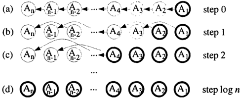
Consider the problem of finding all marginal probabilities, Pr(Aj ) , in the chain network of Figure 2(a), using n pro­ cessors.

n

Processor j is assigned to variable Aj, and "owns" the con­ ditional probability table (CPT) for Pr(Aj IAi _1). Note that processor #1 already holds the marginal probability Pr( A1); it simply records a flag indicating that it is done. At the first time step, each processor j rewrites its CPT in terms of its grandparent, given its own current CPT and its par­ ent's current CPT. Mathematically, processor j computes:

for each combination of values of Aj and Aj _2, taking con­ stant (0(r3)) time. After time step one, processor #2 holds the marginal probability Pr(A2). so it marks itself done (it knows that it is done because its parent was done at the pre­ vious time step). The new network topology after step one is pictured in Figure 2(b). The second time step proceeds exactly as the first-each variable rewrites its CPT in terms of its (new) grandparent:

After time step two, the first four processors hold their re­ spective marginals and mark themselves done. After time step three, the first eight processors are done, etc. Af­ ter log2 n time steps, all n processors are done, and all marginal probabilities have been computed; the entire pro­ cess is conveyed in Figure 2. This procedure of iteratively recomputing CPTs in terms of grandparents is analogous to a widely used method in parallel algorithms to achieve O ( log n ) computations in linked lists, called pointer jump­ ing. In chain networks, the algorithm can operate in an exclusive-read fashion, though we will use concurrent reads later, to process trees and polytrees.

4 INFERENCE IN TREES

This section generalizes PHISHFOOD to compute infer­ ence queries in tree networks. The next subsection begins with computing marginal probabilities only; Section 4.2 presents a parallel arc reversal procedure to propagate ev­ idence.

PHISH-TREE-MARGINALS(T) INPUT: Bayesian network tree T OUTPUT: Pr(Aj) for all j I. mark root node A1 done 2. while there is a node not marked done 3. for each node Aj in parallel 4. compute (1) 5. ifpa(Aj) is marked done 6. then mark Aj done 7. else pa(Aj) +-gp(Aj)

4.1 FINDING MARGINALS IN TREES

Marginal computation in trees proceeds in much the same way as for chains. Again, the central step is for each vari­ able to rewrites its CPT in terms of its grandparent:

Because the graph is a tree, each "set" pa(Aj) and gp(Aj) is actually a singleton. The procedure psuedocode is given in Table I. This simple implementation uses concurrent reads, since each variable may have several grandchildren at a given step. If we consider the root to be at depth one, then, after time step two, all marginals for variables at depth two have been computed; after step three, all marginals at depth four have been computed, etc. All marginals in the tree are computed in O(log d) time, where dis its depth and, in the worst-case, is O(n). Notice that, if the tree is bal­ anced (i.e., is of depth O(logn)), then the running time is O(log log n ) .

4.2 EVIDENCE PROPOGATION IN TREES

This subsection describes how PHISHFOOD propogates evidence, using a parallel version of arc reversal (a form of Bayes's rule), and evidence absorption, the standard ver­ sions of which were developed by Shachter (1988, 1990).

We assume that the graph topology is given as an ad jacency list, so that each node has pointers to its children as well as to its parent. We utilize a standard parallel subroutine that finds a preorder walk of a tree, starting from any given root node. A preordering numbers the nodes according to the order that they are first reached in a depth-first traver­ sal of the underlying undirected tree. The computation can be done in O(log n) time with n processors, using what is called the Euler tour technique (Gibbons and Spirakis 1993; Ja.Ja 1992; Tarjan and Vishkin 1985).

In Bayesian networks, any edge can be reversed such that the transformed network represents the same underlying joint distribution, as ,long the reversal does not create a di­ rected cycle. When an edge between A; and Aj is reversed, both variables must share each other's parents, which, in general, may add significantly to the number of arcs in the graph. However, a tree can be rerooted at any node with­ out adding any arcs. Consider rerooting the tree at the first evidence variable, Ae,. Let a be a preorder walk of the un­ derlying undirected tree, starting from Ae 1· Then a encodes the desired new edge directions-that is, an edge in the re­ rooted tree points from Aa, to a neighbor A"i if and only if a; < a i . A serial arc reversal procedure would begin at the original root A1, which has no parent, reversing any of A1 's child arcs inconsistent with a. A1 's children have no parents other than A1 itself, and thus no new arcs are cre­ ated. Next, any child arcs from ch( A1) inconsistent with a are reversed, then any child arcs from ch( ch(Al) ) , etc. The result is a new tree, rooted at Ae,, with the same underlying undirected topology as the original tree.

Suppose that all marginal probabilities are known, com­ puted as in Section 4.1. Then, since the tree topology is invariant, it is not necessary to reverse arcs in any partic­ ular order. We can simply reverse any edges inconsistent with a simultaneously, in constant parallel time, by apply­ ing Bayes's rule. To be concrete, assign one processor to every edge (since the graph is a tree, there are n -1 edges). If an arc from A; to Aj is inconsistent with the ordering a, then the processor reads the CPT associated with Aj and rewrites the CPT associated with A; according to Bayes's rule:

Since the original and new structures are both trees, each processor reads from and writes over at most one CPT, and each CPT is rewritten by at most one processor.

In general, evidence absorption (Shachter 1988; Shachter 1990) involves a single update at each of Ae, 's children, and a series of arc reversals propagating to all of Ae, 's an­ cestors. However, by construction, the evidence variable is the root and has no ancestors. Each of Ae, 's children Aj simply absorbs the evidence in constant time, with the up­ date:

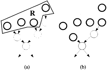
Next, all of Ae, 's child arcs are eliminated, creating dis­ connected trees rooted at each of Ae, 's children. The ev­ idence propagation and absorption process is depicted in Figure 3. The implicit marginal probabilities in these new trees are actually posterior probabilities, given the evidence Ae, = ae,, in the original representation. Note that evi­ dence given in the form of a likelihood function could also be absorbed at Ae,; in this case, Ae, 's child arcs would in general not be eliminated. The algorithm repeats by com­ puting the new marginals as described in Section 4.1, re­ rooting the tree at Ae2, and absorbing the second evidence

.-

,

-,,

Figure 3: Propagating Evidence in a Tree Network. (a) The initial tree. (b) A preordering a of nodes, starting from A e , , with inconsistent arcs reversed. (c) Evidence at the new root, Ae,, is absorbed.

PHISHFOOD-TREE(T, E)

INPUT: Bayesian network tree T, adjacency list, and c evidence variables and values: E = { A e, = a e,, . . . , Aec = a ec } OUTPUT: Pr(Ai IE) for all j 1. PHISH-TREE-MARGINALS(T) 2. for each evidence variable A e k 3. a +PREORDER(T, Aek) 4. for each edge (A;, Aj) in parallel 5. if (A;, A1) is inconsistent with a then 6. compute (2) and store in A; 's CPT 7. absorb evidence (3) at new root A e k 8. PHISH-TREE-MARGINALS(T)

variable, etc. The full psuedocode is given in Table 2. For any constant number of evidence variables, its running time is O ( log n ) with n processors.

5 INFERENCE IN POLYTREES

This section describes a parallel algorithm for Bayesian in­ ference in polytree networks. Once again, discussion is di­ vided into two stages: (1) computing marginal probabili­ ties, and (2) propogating evidence.

5.1 FINDING MARGINALS IN POLYTREES

In trees, PHISHFOOD's key to parallelization is for each variable to iteratively rewrite its CPT in terms of its grand­ parent. In polytrees, a node may have more than one parent, each of which has more than one parent, etc. Since CPT size is exponential in the number of parents, a simple applica­ tion of PHISH-TREE-MARGINALS would be worst-case in­ tractable, so a modified approach is necessary.

The structure of a polytree implies many independencies between variables, which can be exploited to speed infer­ ence (Neapolitan 1990; Pearl 1988; Russell and Norvig 1995). In particular, given no evidence at A1, or at any of Aj 's descendents, the parents of A1 are independent. That is, if A;, and A;2 are both parents of A1, then Pr(A;, A;2IE) = Pr(A;, IE) Pr(A;2IE), for any set of evidence variables E that does not contain A1 or any of Aj 's descendents. Consider an arbitrary node A1. If its parents' marginal probabilities are known, then, since its parents are independent, Ai 's marginal can be computed. Similarly, its parents' marginals can be computed once its grandparents' marginals are known. Let A1 's induced ancestral polytree 2 (lAP) be the subnetwork induced by Ai and its ancestors-that is, the network consisting of AJ, pa(AJ ), pa(pa(AJ )), pa(pa(pa(Aj ))) , etc., and the edges between them. Note that this subnetwork contains all of the necessary information to compute Pr ( A1).

I will make use of the following terms: a polynode is a vari­ able with more than one parent, a treenode is a variable with exactly one parent, and a rootnode is a variable with no par­ ents.

I adopt a strategy similar in style to that employed in Miller and Reif's parallel tree contraction algorithm (1985). The algorithm consists of two main steps: the first is called root­ node absorption (analogous to Miller and Reif's RAKE pro­ cedure), and the second is treenode jumping (analogous to their COMPRESS procedure). The main conceptual diffi­ culty in directly mapping the current problem to parallel tree contraction is that each node can have both multiple parent and multiple child relationships, each with very dif­ ferent semantics. The key insight is that each node's lAP can be contracted in more or less the standard way, by ex­ ploiting the independence properties mentioned above.

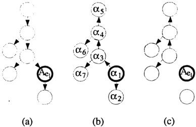
We initialize the algorithm by marking all rootnodes as done. In the first step, each node absorbs all of its rootnode parents (if any) in constant parallel time. Consider node A1. Denote Rj = {A;,, ... , A;.} as the set of A1 's rootnode parents, and Ii as the set of Aj 's other, internal node par­ ents (thus pa(Aj) = Rj U Ij ). Then the update at A1 is as follows:

where 'L: R _ is the sum over all combinations of values of ) the variables in Rj, and the equality follows from the independence properties of a polytree. Any new rootnodes that are formed after absorption now hold their marginal prob­ abilities, and are marked as done. This first phase is illus­ trated in Figure 4.

2 Indiscriminate use of this phrase discouraged.

Iterative application of rootnode absorption alone would require 0( n ) time to compute all marginals in an unbal­ anced polytree. We interleave the second step-treenode jumping-to compress long treenode chains in the network. We accomplish this with one step of the pointer jumping procedure described in section 3, applied only at treenodes. That is, each treenode CPT is rewritten in terms of its grand­ parent(s) by computing (1). Since treenodes have exactly one parent, this step does not introduce a combinatorial growth in parent set size. This step will essentially reduce the length of treenode chains in each lAP by half. As be­ fore, if the treenode's parent is marked done at time step t -1, then the treenode itself can be marked done at time step t. This second phase is pictured in Figure 5. After both phases, the algorithm iterates on the transformed polytree: we absorb each new rootnode, rewrite each new treenode CPT in terms of its grandparent(s), and repeat until all nodes are marked done. The algorithm psuedocode is given in Ta­ ble 3.

For the time complexity analysis, we show that, for each node, the number of "active" nodes (those not marked done) in its induced ancestral polytree (lAP) is reduced by at least half at each iteration. Consider Aj 'slAP at time step t1, consisting of rootnodes R, treenodes T, and polynodes P. Note that because the network is acyclic, I P I :::; I R I . (Each

PHISH-POLY-MARGINALS(P) INPUT: Bayesian network polytree P OUTPUT: Pr(Aj) for all j

1. mark all rootnodes done
2. while there is a node not marked done
3. for each node Aj with rootnode parent(s) in parallel
4. absorb rootnode parents (4)
5. if Aj has no more parents
6. then mark Aj done
7. for each treenode Aj in parallel
8. compute (1)
9. then mark Aj done
10. if pa( Aj) is marked done
11. else pa( Aj) <----gp( Aj)
12. identify new rootnodes, treenodes, polynodes

Table 3: Computing all Marginal Probabilities a Polytree Network.

polynode implies a path between at least two rootnodes; if there are more polynodes than rootnodes, then there must be a cycle in the lAP.) At time step t, Aj 's new lAP consists of the nodes T' U P', where T' � T, and P' � P, since all rootnodes have been absorbed. For each node in T', exactly one node in T UP has been "jumped", and is thus no longer in Aj 's lAP. Thus, I T' I = I T I - I T' I + I P I - I P' I . Combin­ ing this equality with the previous inequality, we find that:

Thus, after O(log n ) iterations, each node's lAP is reduced to a singleton, and all marginals have been computed.

5.2 EVIDENCE PROPAGATION IN POLYTREES

As with trees, evidence is propagated with arc reversals. The first step is to convert the polytree into a directed cluster polytree, as described in Section 2. Since the moral graph of a polytree is triangulated, the supernodes simply consist of each variable and its parents, and the cluster polytree's size is of the same order as the original polytree. A clus­ ter tree, like an ordinary tree, can be rooted at any node, without changing its underlying undirected topology (Chyu 1991; Shachter, Andersen, and Poh 1991 ) . Once all margi­ nal probabilities are known, we can root the cluster tree with the method described in Section 4.2 in O(log n ) time. The algorithm PHISHFOOD-TREE is then applicable, unmodi­ fied, for inference in the rooted cluster tree.

6 INFERENCE IN ARBITRARY NETWORKS

In the general case, we first convert to a directed cluster polytree, as described in Section 2. The parallel inference algorithm, called McPHISHFOOD (Multiply Connected PHISHFOOD) is exactly that for polytrees, and has a new acronym only to accommodate any future corporate spon­ sorship.

Assuming that the fill-in ordering a is chosen with a heuris­ tic method, all of the graph-theoretic computations can be done in polynomial time. Consider the complexity of com­ puting the supernodes' CPTs. After separation sets are in­ troduced, each supernode CPT contains 0( rw ) entries, and each entry is computed by multiplying w of the original CPTs' entries. For this task, parallelization is trivial. Each entry of each supernode CPT can be computed indepen­ dently, taking 0( rw w ) time with one processor per clique, or O(log w ) time with rw w processors per clique. 3

In both the tree and polytree algorithms, the complexity bot­ tleneck is (1), because this computation involves three su­ pernodes. The summation is evaluated for each possible combination of values of Ci and gp( Ci ) . A conservative bound for computing the new CPT is 0( r3w ) time with one processor, or O(log rw) = 0( w ) time with r3w proces­ sors. We can do slightly better by exploiting separation sets. First, each separation set CPT is rewritten in terms of its separation set grandparent(s), taking O (rw) time with one processor, or 0(1) time with rw processors. The marginal­ finding algorithm is then applied only to the network of sep­ aration sets. Once all separation set marginals are known, remaining marginals can be computed in O(rw) or 0(1) time, with one or rw processors, respectively.

Any cluster tree can be rooted at any of its cliques, without changing its topology (Chyu 1991; Shachter, Andersen, and Poh 1991). For each evidence variable, we root the clus­ ter tree at the supernode that contains it. Each application of Bayes's rule (2) takes O(rw) time with one processor, or 0(1) time with rw processors. Evidence is absorbed at the new root by instantiating the variable, then renormaliz­ ing the remaining constituents of the supernode, in 0( rw ) or 0( w ) time, with one or rw processors, respectively.

The full McPHISHFOOD algorithm then runs in 0( r3w log n) time with n processors, or 0( w log n) time with r3wn processors, for any constant number of evidence variables. Let s be the maximum separation set size. If we exploit separation sets as described above, then inference takes 0( r3· log n ) time with one processor, or O(w+s log n) time with r3·n processors. These improved bounds assume that 3s > w.

3 Multiplication (or addition) of m numbers can be done in O(log m ) parallel time with m processors.

7 RELATED WORK

D'Ambrosio ( 1992) examines the possibility of paralleliz­ ing the symbolic probabilistic inference (SPI) algorithm on hypercube parallel architectures. He identifies two sources of concurrency: topological or "evaluation tree" paral­ lelism, and conformal product parallelism; in the former case, he only considers exploiting independent computa­ tions, stating that, "a lower bound on the running time of an algorithm exploiting evaluation tree parallelism can be calculated by summing the [computations] in the longest path of the evaluation tree." Given several different mod­ eling assumptions, he empirically evaluates predicted com­ putational, communication, and storage costs, and parallel speedup and efficiency. He concludes that good opportuni­ ties exist for parallelizing independent conformal products evaluations, but not much natural concurrency is present at the topological level.

Kozlov and Singh (1996, 1994) describe experimental re­ sults for a parallel version of a junction tree algorithm, im­ plemented on a Stanford DASH multi-processor and an SGI Challenge XL. They identify the same two types of con­ currency (topological and in-clique), and also only consid­ ered parallelizing independent operations: "computations for cliques that do not have an ancestor-descendent relation­ ship can be done in parallel." (Kozlov 1996).

Deicher et al. (1996) give an O(log n ) time serial algorithm for inference queries in tree networks, after a linear time preprocessing step to generate a special data structure. This data structure is actually based on the tree contraction se­ quence described by Abrahamson et al. in the context of a parallel algorithm (1989).

8 CONCLUSION AND FUTURE WORK

I have presented PHISHFOOD, a parallel algorithm for ex­ act Bayesian inference that, for any constant number of ev­ idence variables, runs in O(Iog n) time for polytrees, and 0( r3w log n) time for cluster trees with n processors, and 0( w log n) time for cluster trees with r3w n processors. Concurrent memory reads, but not writes, are required.

There are several possible directions for improving the al­ gorithm. An O(log n ) exclusive-read polytree algorithm may be possible, perhaps based on Abrahamson et al.'s EREW parallel tree contraction algorithm (1989).4 The work done by an algorithm is defined as its running time multiplied by the number of processors used. There may exist a work-efficient version of PHISHFOOD that uses only n / log n processors.

Future work might also pursue parallelizations for other

4Any CREW (or CRCW) algorithm can run on an EREW PRAM with an O(log n) factor slowdown. (Cormen, Leiserson, and Rivest 1992; Gibbons and Spirakis 1993; JaJa 1992)

types of inference queries (e.g., most probable explanation, maximum expected utility, value of information), and for other conditional probability encodings (e.g., noisy-OR).

Certainly, an implementation of these algorithms is called for, on a specific parallel architecture, along with empirical comparisons with existing serial and parallel algorithms.

Acknowledgments

Thanks to David Pynadath and to the anonymous reviewers.

References

• Abrahamson, K., N. Dadoun, D. G. Kirkpatrick, and T. Przyttycka (1989). A simple parallel tree contrac­ tion algorithm. Journal of Algorithms 10, 287-302.
• Chyu, C. C. (1991). Decomposable probabilistic influ­ ence diagrams. Probability in the Engineering and Informational Sciences 5, 229-243.
• Cooper, G. (1990). The computational complexity of probabilistic inference using Bayes belief networks. Artificial Intelligence 42, 393-405.
• Cormen, T. H., C. E. Leiserson, and R. L. Rivest (1992). Introduction to Algorithms. New York: McGraw­ Hill.
• Dagum, P. and M. Luby (1993). Approximating proba­ bilistic inference in Bayesian belief networks is NP­ hard. Arti ficial Intelligence 60, 141-153.
• D'Ambrosio, B. ( 1992). Parallelizing probabilistic infer­ ence: Some early explorations. In Proceedings of the Eighth Conference on Uncertainty in Artificial Intel­ ligence (UAI-92), Portland, OR, USA, pp. 59-66.
• Deicher, A. L., A. J. Grove, S. Kasif, and J. Pearl (1996, February). Logarithmic-time updates and queries in probabilistic networks. Journal of Artificial Intelli­ gence Research 4, 37-59.
• Diez, F. J. and J. Mira (1994, January). Distributed in­ ference in Bayesian networks. Cybernetics and Sys­ tems 2 5( 1 ), 39-61.
• Gibbons, A. and P. Spirakis (1993). Lectures on Paral­ lel Computation. Cambridge, UK: Cambridge Uni­ versity Press.
• Ja.Ja, J. (1992). An Introduction to Parallel Algorithms. Reading, MA, USA: Addison-Wesley.
• Jensen, F. V., S. L. Lauritzen, and K. G. Olesen (1990). Bayesian updating in causal probabilistic networks by local computations. Computational Statistics Quarterly 4, 269-282.
• Klocks, T. (1994). Treewidth: Computations and Ap­ proximations. Berlin: Springer-Verlag.
• Kozlov, A. V. (1996, December). Parallel implementa­ tions of probabilistic inference. Computer 29 (12 ), 33-40.
• Kozlov, A. V. andJ. P. Singh (1994, November). A paral­ lel Lauritzen-Spiegelhalter algorithm for probabilis­ tic inference. In Proceedings of Supercomputing '94, Washington, DC.
• Lauritzen, S. L. and D. J. Spiegelhalter (1988). Local computations with probabilities on graphical struc­ tures and their application to expert systems. Jour­ nal of the Royal Statistical Society, Series B 50, 157224.
• Miller, G. L. and J. Reif (1985). Parallel tree contrac­ tion and its applications. In Proceedings of the 26th IEEE Symposium on Foundations of Computer Sci­ ence, pp. 478-489.
• Neapolitan, R. E. (1990). Probabilistic Reasoning in Ex­ pert Systems: Theory and Algorithms. New York: John Wiley and Sons.
• Pearl, J. (1988). Probabilistic Reasoning in Intelligent Systems. Morgan Kaufmann.
• Russell, S. J. and P. Norvig (1995). Arti ficial Intelli­ gence: A Modem Approach. New Jersey: Prentice­ Hall.
• Shachter, R. D. (1988). Probabilistic inference and in­ fluence diagrams. Operations Research 36(4), 589604.
• Shachter, R. D. (1990). Evidence absorption and prop­ agation through evidence reversals. In M. Henrion, R. D. Shachter, L. N. Kanal, and J. F. Lemmer (Eds.), Uncertainty in Artificial Intelligence, Volume 5, pp. 173-190. North Holland.
• Shachter, R. D., S. K. Andersen, and K. L. Poh (1991). Directed reduction algorithms and decomposable graphs. In P. P. Bonissone, M. Henrion, L. N. Kanal, and J. F. Lemmer (Eds.), Uncertainty in Artificial Intelligence, Volume 6, pp. 197-208. Amsterdam: North Holland.
• Shachter, R. D., S. K. Andersen, and P. Szolovits (1994). Global conditioning for probabilistic inference in be­ lief networks. In Proceedings of the Tenth Confer­ ence on Uncertainty in Artificial Intelligence (UAI94), Portland, OR, USA, pp. 514-522.
• Spiegelhalter, D. J., A. P. Dawid, S. L. Lauritzen, and R. G. Cowell (1993). Bayesian analysis inexpert sys­ tems. Statistical Science 8(3), 219-203.
• Tarjan, R. E. and U. Vishkin (1985, November). An ef­ ficient parallel biconnectivity algorithm. SIAM Jour­ nal on Computing 14(4), 862-874.