Multi-objective Influence Diagrams ∗

Radu Marinescu

IBM Research - Ireland [email protected]

Abstract

We describe multi-objective influence diagrams, based on a set of p objectives, where utility values are vectors in R p , and are typically only partially ordered. These can still be solved by a variable elimination algorithm, leading to a set of maximal values of expected utility. If the Pareto ordering is used this set can often be prohibitively large. We consider approximate representations of the Pareto set based on /epsilon1 -coverings, allowing much larger problems to be solved. In addition, we define a method for incorporating user tradeoffs, which also greatly improves the efficiency.

1 INTRODUCTION

Influence diagrams [1] are a powerful formalism for reasoning with sequential decision making problems under uncertainty. They involve both chance variables, where the outcome is determined randomly based on the values assigned to other variables, and decision variables, which the decision maker can choose the value of, based on observations of some other variables. Uncertainty is represented (like in a Bayesian network) by a collection of conditional probability distributions, one for each chance variable. The overall value of an outcome is represented as the sum of a collection of utility functions.

In many situations, a decision maker has more than one objective, and mapping several objectives to a single utility scale can be problematic, since the decision maker may be unwilling or unable to provide precise tradeoffs between objectives [2, 3, 4]. We consider multi-objective influence diagrams, where utility values are now vectors in R p , with p being the number of objectives. Since utility values are

∗ Abdul Razak is funded by IRCSET and IBM through the IRCSET Enterprise Partnership Scheme. This work was also supported in part by the Science Foundation Ireland under grant no. 08/PI/I1912

Abdul Razak and Nic Wilson Cork Constraint Computation Centre University College Cork, Ireland

{ a.razak,n.wilson } @4c.ucc.ie now only partially ordered (for instance by the Pareto ordering) we no longer have a unique maximal value of expected utility, but a set of them.

The Pareto ordering on multi-objective utility is a rather weak one; the effect of this is that the set of maximal values of expected utility can often become huge. We discuss how the notion of /epsilon1 -covering, which approximates the Pareto set, can be applied for the case of multi-objective influence diagrams. As we demonstrate experimentally, this has a major effect on the size of the undominated utility vector sets and hence on the computational efficiency and feasibility for larger problems.

We also define a simple formalism for imprecise tradeoffs; this allows the decision maker, during the elicitation stage, to specify a preference for one multi-objective utility vector over another, and uses such inputs to infer other preferences. The induced preference relation then is used to eliminate dominated utility vectors during the computation. Our experimental results indicate that the presence of even a few such imprecise tradeoffs greatly reduces the undominated set of expected utility values.

The paper is organized as follows. We first discuss the related work. Then Section 2 describes standard influence diagrams and multi-objective utility values. Section 3 defines multi-objective influence diagrams, and how variable elimination can be used to compute the set of maximal values of expected utility, up to a form of equivalence. Section 4 describes the use of the /epsilon1 -covering of the Pareto set. Section 5 defines the formalism for tradeoffs and how the induced notion of preference dominance can be computed. Section 6 describes our experimental testing of multi-objective influence diagrams, based on the Pareto ordering, on the /epsilon1 -covering approximation, and based on the dominance relation induced by the user tradeoffs. Section 7 concludes.

RELATED WORK: Our approach to multi-objective influence diagram computation is based on our general framework [5].

Diehl and Haimes [6] describe a computational technique for influence diagrams with multiple objectives, with the restriction of just a single value node (utility function). The solution method is based on influence diagram transformations [7]. Pareto dominance is used to prune sub-optimal utility vectors during the computation (with tradeoffs being taken into account at the end of the computation).

Papadimitriou and Yannakakis [8] proposed the use of the logarithmic grid in (1 + /epsilon1 ) to generate an /epsilon1 -covering of the Pareto set. Dubus et al. [9] also developed a variable elimination algorithm that uses /epsilon1 -dominance over a graphical model (GAI network) that represents a (multi-objective) generalized decomposable additive utility function.

Zhou et al. [10] consider influence diagrams (with a unique value node) based on interval-valued utility, which is similar to bi-objective utility. They adapt Cooper's approach for solving influence diagrams based on Bayesian network algorithms [11]. Other extensions of influence diagrams include work in [12, 13, 14] which allow interval probability (but precise single-objective utility), and in [15] which considers generalized influence diagrams based on fuzzy random variables.

Maua et al. [16] proposed a variable elimination algorithm for solving Limited Memory Influence Diagrams (LIMIDs). Although they consider standard totally ordered utilities, their algorithm also manipulates partially ordered sets: in their case, sets of functions that are used to represent the effect of different undominated policies.

Our method for incorporating tradeoffs relates to convex cones , as shown by Theorem 3. A general approach to multi-objective preferences based on cones has been developed by Yu and others [17, 18].

2 BACKGROUND

2.1 INFLUENCE DIAGRAMS

An influence diagram (ID) [1] is defined by a tuple 〈 X , D , P , U 〉 , where X = { X 1 , . . . , X n } is a set of chance variables which specify the uncertain decision environment and D = { D 1 , . . . , D m } is a set of decision variables which specify the possible decisions to be made in the domain. The chance variables are further divided into observable meaning they will be observed during execution, or unobservable . As in Bayesian networks [19], each chance variable X i ∈ X is associated with a conditional probability table (CPT) P i = P ( X i | pa ( X i )) , where P i ∈ P and pa ( X i ) ⊆ X ∪ D \ { X i } . Each decision variable D k ∈ D has a parent set pa ( D k ) ⊆ X ∪ D \ { D k } , denoting the variables whose values will be known at the time of the decision and may affect directly the decision. Non-forgetting is typically assumed for an influence diagram, meaning that a decision node and its parents are parents to all subsequent decisions. The utility (or reward ) functions U = { U 1 , . . . , U r } are defined over subsets of

variables Q = { Q 1 , . . . , Q r } , Q i ⊆ X ∪ D , called scopes , and represent the preferences of the decision maker.

The graph of an ID contains nodes for chance variables (circled), decision variables (boxed) and for the utility components (diamond). For each chance or decision node there is an arc directed from each of its parent variables toward it, and there is a directed arc from each variable in the scope of a utility function toward its utility node.

The decision variables in an influence diagram are typically assumed to be temporally ordered (also known as regularity ). Let D 1 , D 2 , ..., D m be the order in which the decisions are to be made. The chance variables can be partitioned into a collection of disjoint sets I 0 , I 1 , . . . , I m . For each k , where 0 < k < m , I k is the set of chance variables that are observed between D k and D k +1 . I 0 is the set of initial evidence variables that are observed before D 1 . I m is the set of chance variables left unobserved when the last decision D m is made. This induces a strict partial order ≺ over X ∪ D , given by: I 0 ≺ D 1 ≺ I 1 ≺ · · · ≺ D m ≺ I m [20].

A policy (or strategy ) for an influence diagram is a list of decision rules ∆ = ( δ 1 , . . . , δ m ) consisting of one rule for each decision variable. A decision rule for the decision D k ∈ D is a mapping δ k : Ω pa ( D k ) → Ω D k , where for a set S ⊆ X ∪ D , Ω S is the Cartesian product of the individual domains of the variables in S . Therefore, a policy ∆ determines a value for each decision variable D i (which depends on the parents set pa ( D i ) ). Given a utility function U , a policy ∆ yields a utility function [ U ] ∆ that involves no decision variables, by assigning their values using ∆ . The expected utility given policy ∆ is EU ∆ = ∑ X [( ∏ n i =1 P i × ∑ r j =1 U j )] ∆ . Solving an influence diagram means finding an optimal policy that maximizes the expected utility, i.e., to find arg max ∆ EU ∆ . The maximum expected utility can be shown to be equal to:

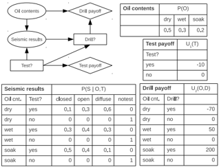
Example 1 Figure 1 shows the influence diagram of the oil wildcatter problem (adapted from [21]). An oil wildcatter must decide either to drill or not to drill for oil at a specific site. Before drilling, a seismic test could help determine the geological structure of the site. The test results can show a closed reflection pattern (indication of significant oil), an open pattern (indication of some oil), or a diffuse pattern (almost no hope of oil). The special value notest is used if no seismic test is performed. There are therefore two decision variables, T (Test) and D (Drill), and two chance variables S (Seismic results) and O (Oil contents). The probabilistic knowledge consists of the conditional probability tables P ( O ) and P ( S | O,T ) , while the utility function is the sum of U 1 ( T ) and U 2 ( O,D ) . The optimal policy is to perform the test and to drill only if the test results show an open or a closed pattern. The expected utility of this policy is 22.5.

Several exact methods have been proposed over the past decades for solving influence diagrams using local computations [7, 22, 23, 20, 24, 25]. These methods adapted classical variable elimination techniques, which compute a type of marginalization over a combination of local functions, in order to handle the multiple types of information (probabilities and utilities), marginalization ( ∑ and max ) and combination ( × for probabilities, + for utilities) involved in influence diagrams. Since the alternation of ∑ and max in Equation 1 does not commute in general, it prevents the solution technique from eliminating variables in any ordering. Therefore, the computation dictated by Equation 1 must be performed along a legal elimination ordering that respects ≺ , namely the reverse of the elimination ordering is some extension of ≺ to a total order [20, 24].

2.2 MULTI-OBJECTIVE UTILITY VALUES

In many real-world situations it may not be possible for the decision maker to map the various possible consequences of a set of actions to the same scale of utility in a way that avoids essentially arbitrary decisions. Hence, it is natural to consider multi-objective or multi-attribute utility functions to cope with multiple and non-commensurate utility scales on which the decision maker's preferences are expressed.

Consider a situation with p objectives (or attributes). A multi-objective utility value is characterized by a vector /vector u = ( u 1 , . . . , u p ) ∈ R p , where u i represents the utility with respect to objective i ∈ { 1 , . . . , p } . We assume the standard pointwise arithmetic operations, namely /vector u + /vector v = ( u 1 + v 1 , . . . , u p + v p ) and q × /vector u = ( q × u 1 , . . . , q × u p ) , where q ∈ R . The comparison of utility values reduces to that of their corresponding p -dimensional vectors.

We are interested in partial orders /followsorcurly on R p satisfying the following two monotonicity properties, where /vector u,/vector v, /vector w ∈ R p are arbitrary vectors.

[Independence:] If /vector u /followsorcurly /vector v then /vector u + /vector w /followsorcurly /vector v + /vector w

[Scale-Invariance:] If /vector u /followsorcurly /vector v and q ∈ R , q ≥ 0 then q × /vector u /followsorcurly q × /vector v .

An important example of such a partial order is the weak Pareto order.

DEFINITION 1 (weak Pareto ordering) Let /vector u,/vector v ∈ R p such that /vector u = ( u 1 , . . . , u p ) and /vector v = ( v 1 , . . . , v p ) . We define the binary relation ≥ on R p by /vector u ≥ /vector v ⇐⇒ ∀ i ∈ { 1 , . . . , p } u i ≥ v i .

Given /vector u,/vector v ∈ R p , if /vector u /followsorcurly /vector v then we say that /vector u dominates /vector v . As usual, the symbol /follows refers to the asymmetric part of /followsorcurly , namely /vector u /follows /vector v if and only if /vector u /followsorcurly /vector v and it is not the case that /vector v /followsorcurly /vector u . In particular, relation ≥ (resp. > ) is also called weak Pareto dominance (resp. Pareto dominance ).

DEFINITION 2 (maximal/Pareto set) Given a partial order /followsorcurly and a finite set of utility vectors U ⊆ R p , we define the maximal set , denoted by max /followsorcurly ( U ) , to be the set consisting of the undominated elements in U , i.e., max /followsorcurly ( U ) = { /vector v ∈ U | /notexistential /vector v ∈ U , /vector v /follows /vector u } . When /followsorcurly is the weak Pareto ordering ≥ , we call max /followsorcurly ( U ) the Pareto set .

3 MULTI-OBJECTIVE INFLUENCE DIAGRAMS

In this section, we introduce the extension of the standard influence diagram model to include multiple objectives. Towards this goal we consider a multi-objective utility function that is additively decomposable [26]. For simplicity and without loss of generality we assume that all objectives are to be maximized. We next define formally the graphical model and then derive a sequential variable elimination algorithm for evaluating the model.

3.1 THE GRAPHICAL MODEL

A multi-objective influence diagram (MOID) extends the standard influence diagram by allowing a multi-objective utility function defined on p > 1 objectives. The graphical structure of a MOID is identical to that of a standard ID, namely it is a directed acyclic graph containing chance nodes (drawn as circles) for the random discrete variables X , decision nodes (drawn as rectangles) for the decision variables D , and utility nodes (drawn as diamonds) for the local utility functions U of the decision maker. The directed arcs in the MOID represent the same dependencies between the variables as in the standard model. Each chance node X i ∈ X is associated with a conditional probability table P ( X i | pa ( X i )) : Ω X i ∪ pa ( X i ) → [0 , 1] . The utility functions U j ∈ U represent the decision maker's preferences with respect to each of the p objectives, namely U j : Ω Q j → R p , where Q j is the scope of U j .

A policy for a MOID is a sequence ∆ = ( δ 1 , . . . , δ m ) , where each δ i is a function from Ω pa ( D i ) → Ω D i . Clearly, given a policy ∆ we have that EU ∆ ⊆ R p . Solving a multi-objective influence diagram means finding the set of

policies that generate maximal values of expected utility, i.e., values of utility in the set max /followsorcurly { EU ∆ | policies ∆ } . We say that a policy ∆ is optimal if the corresponding expected utility EU ∆ is undominated.

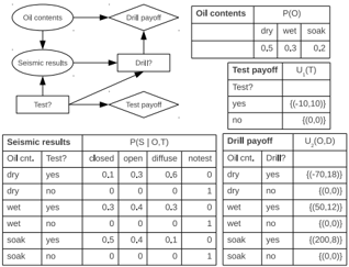
Example 2 Figure 2 displays a bi-objective influence diagram for the decision problem from Example 1. We consider a utility function with two attributes representing the testing/drilling payoff and damage to the environment, respectively. The utility of testing is ( -10 , 10) , whereas the utility of drilling is ( -70 , 18) , (50 , 12) , (200 , 8) for a dry, wet and soaking hole, respectively. The aim is to find optimal policies that maximize the payoff and minimize the damage to environment. The dominance relation is defined in this case by /vector u ≥ /vector v ⇔ u 1 ≥ v 1 and u 2 ≤ v 2 (e.g., (10 , 2) ≥ (8 , 4) and (10 , 2) /notgreaterequal (8 , 1) ). The Pareto set max ≥ { EU ∆ | policies ∆ } contains 4 elements, i.e., { (22 . 5 , 17 . 56) , (20 , 14 . 2) , (11 , 12 . 78) , (0 , 0) } , corresponding to the four optimal policies shown below (we show how to obtain these in Section 3.4):

	∆ 1	∆ 2	∆ 3	∆ 4
δ T	yes	no	yes	no
δ D	yes (S = closed) yes (S = open) no (S = diffuse)	yes (S = notest)	yes (S = closed) no (S = open) no (S = diffuse)	no (S = notest)

EU ∆ i { (22 . 5 , 17 . 56) } { (20 , 14 . 2) } { (11 , 12 . 78) } { (0 , 0) }

Because we are considering partially ordered utilities, the max operator does not necessarily lead to a unique element. This means that we need to extend the arithmetic operations, addition, multiplication and max , to finite sets of utility values.

3.2 ARITHMETIC OPERATIONS AND DISTRIBUTIVITY PROPERTIES

In this section we assume a partial order /followsorcurly on R p that satisfies Independence and Scale-Invariance. In particular, /followsorcurly can be the weak Pareto ordering.

Given two finite sets U , V ⊆ R p and q ≥ 0 , we define the summation and multiplication operations as U + V = { /vector u + /vector v | /vector u ∈ U , /vector v ∈ V} and q × U = { q × /vector u | /vector u ∈ U} , respectively. The maximization operation is defined as max( U , V ) = max /followsorcurly ( U ∪ V ) . It is easy to see that + , × and max are commutative and associative.

To ensure the correctness of a variable elimination computation (such as the one in Algorithm 1) we need some distributivity properties. However, the important property ( q 1 + q 2 ) ×U = q 1 ×U + q 2 ×U does not always hold. As a simple example, let q 1 = q 2 = 0 . 5 and consider a set of bi-objective utility vectors U = { (1 , 0) , (0 , 1) } . Using the point-wise operations on pairs of real numbers we have that ( q 1 + q 2 ) × U yields the set { (1 , 0) , (0 , 1) } , whereas ( q 1 × U ) + ( q 2 × U ) = { (0 . 5 , 0) , (0 , 0 . 5) } + { (0 . 5 , 0) , (0 , 0 . 5) } = { (1 , 0) , (0 . 5 , 0 . 5) , (0 , 1) } . We will see next that this distributivity property does hold if we restrict to convex sets.

3.3 EQUIVALENT SETS OF UTILITY VALUES

For U , V ⊆ R p , we say that U /followsorcurly V if every element of V is (weakly) dominated by some element of U (so that U contains as least as large elements as V ), namely if for all /vector v ∈ V there exists /vector u ∈ U with /vector u /followsorcurly /vector v . We also define an equivalence relation ≈ between two finite sets U , V ⊆ R p by U ≈ V if and only if U /followsorcurly V and V /followsorcurly U .

Given a set U ⊆ R p , we define its convex closure C ( U ) to consist of every element of the form ∑ k j =1 ( q j × /vector u j ) , where k is an arbitrary natural number, each /vector u j ∈ U , each q j ≥ 0 and ∑ k j =1 q j = 1 , respectively.

Given U , V ⊆ R p , we define the equivalence relation ≡ by U ≡ V if and only if C ( U ) ≈ C ( V ) . Therefore, two sets of utility vectors are considered equivalent if, for every convex combination of elements of one, there is a convex combination of elements of the other which is at least as good (with respect to the partial order /followsorcurly on R p ). The following result shows, in particular, that the operations on sets of utility values respects the equivalence relation.

PROPOSITION 1 Let U , V , W ⊆ R p be finite sets and let q ≥ 0 . The following properties hold: (1) U ≡ max /followsorcurly ( U ) ; (2) if U ≡ V then q ×U ≡ q ×V , U + W ≡ V + W and max( U , W ) ≡ max( V , W ) .

We can show now that the distributivity, and other properties we require, hold with respect to the ≡ relation between finite sets of partially ordered utility values.

THEOREM 1 Let /followsorcurly be a partial order on R p satisfying Independence and Scale-Invariance. Then, for all q, q 1 , q 2 ≥ 0 and for all finite sets U , V , W ⊆ R p , we have that:

(i) q × ( U + V ) = q ×U + q ×V ;

(ii) ( q 1 + q 2 ) ×U ≡ ( q 1 ×U ) + ( q 2 ×U ) ;

(iii) q 1 × ( q 2 ×U ) = ( q 1 × q 2 ) ×U ;

(iv) max( q ×U , q ×V ) = q × max( U , V ) ;

(v) max( U + W , V + W ) ≡ max( U , V ) + W .

This implies that variable elimination can be used to gen-

Algorithm 1 : ELIM-MOID

Data : A MOID 〈 X , D , P , U 〉 with p > 1 objectives, a legal elimination ordering of the variables τ = ( Y 1 , . . . , Y t ) Result : An optimal policy ∆ // partition the functions into buckets for l = t downto 1 do 1 place in buckets [ l ] all remaining components in P and U 2 that contain variable Y l in their scope // top-down step for l = t downto 1 do 3 let Φ l = { φ 1 , . . . , φ j } and Ψ l = { ψ 1 , . . . , ψ k } be the 4 probability and utility components in buckets [ l ] if Y l is a chance variable then 5 φ l ← ∑ Y l ∏ j i =1 φ i 6 ψ l ← ( φ l ) -1 × ∑ ′ Y l (( ∏ j i =1 φ i ) × ( ∑ k j =1 ψ j )) 7 else if Y l is a decision variable then 8 φ l ← max Y l ∏ j i =1 φ i 9 ψ l ← max Y l (( ∏ j i =1 φ i ) × ( ∑ k j =1 ψ j )) 10 place each φ l and ψ l in the bucket of the highest-index 11 variable in its scope // bottom-up step for l = 1 to t do 12 if Y l is a decision variable then 13 δ l ← arg max Y l (( ∏ j i =1 φ i ) × ( ∑ k j =1 ψ j )) 14 ∆ ← ∆ ∪ δ l 15 return ∆ 16

erate the set of maximal values of expected utility, up to equivalence (see also [5] for more details).

3.4 VARIABLE ELIMINATION

As well as operation + on sets of utilities, we define operation + ′ on finite sets of utility values by U + ′ V = max /followsorcurly ( U + V ) . Theorem 1 allows us to apply an iterative variable elimination procedure along a legal elimination ordering where chance variables are eliminated by + ′ , decision variables by max , and the probability and (set-valued) utility functions are combined by × and + , respectively. The set of maximal expected utility values is equivalent to ∑ ′ I 0 max D 1 · · · max D m ∑ ′ I m ( ∏ n i =1 P i × ∑ r j =1 U j ) .

The variable elimination algorithm, called ELIM-MOID, is described by Algorithm 1. It is based on Dechter's bucket elimination framework [24] and computes the maximal set max /followsorcurly { EU ∆ | policies ∆ } as well as an optimal policy (the algorithm can be easily instrumented to produce the entire set of optimal policies). Given a legal elimination ordering τ = Y 1 , . . . , Y t , the input functions are partitioned into a bucket structure, called buckets , such that each bucket is associated with a single variable Y l and contains all input probability and utility functions whose highest variable in their scope is Y l .

ELIM-MOID processes each bucket, top-down from the last to the first, by a variable elimination procedure that com- putes new probability (denoted by φ ) and utility (denoted by ψ ) components which are then placed in corresponding lower buckets (lines 3-11). For a chance variable Y l , the φ -message is generated by multiplying all probability components in that bucket and eliminating Y l by summation. The ψ -message is computed as the average utility in that bucket, normalized by the bucket's compiled φ (here Y l is eliminated by ∑ ′ ). For a decision variable Y l , we compute the φ and ψ components in a similar manner and eliminate Y l by maximization. In this case, the product of probability components in the bucket is a constant when viewed as a function of the bucket's decision variable and therefore the compiled φ -message is a constant as well [20, 5].

In the second, bottom-up step, the algorithm generates an optimal policy (lines 12-16). The decision buckets are processed in reversed order, from the first variable to the last. Each decision rule is generated by taking the argument of the maximization operator applied over the combination of probability and utility components in the respective bucket, for each combination of the variables in the bucket's scope (i.e., the union of the scopes of all functions in the bucket minus Y l ) while remembering the values assigned to earlier decisions. Ties are broken uniformly at random.

As is usually the case with bucket elimination algorithms, the complexity of ELIM-MOID can be bounded exponentially (time and space) by the width of the ordered induced graph that reflects the execution of the algorithm (i.e., induced width of the legal elimination ordering) [24]. Since the utility values are vectors in R p , it is not easy to predict the size of the undominated set of expected utility values.

4 APPROXIMATING THE PARETO SET

In this section, we assume without loss of generality a weak Pareto ordering on R p + because the proposed approximation method relies on a log transformation of the solution space as we will see next. The cardinality of the Pareto set max ≥ { EU ∆ : policies ∆ } (and also the number of optimal policies) can often get very large. What would then be desirable for the decision maker is an approximation of the Pareto set that approximately dominates (or covers) all elements in { EU ∆ : policies ∆ } and is of considerably smaller size. This can be achieved by considering the notion of /epsilon1 -covering of the Pareto set which is based on /epsilon1 -dominance between utility values [8].

DEFINITION 3 ( /epsilon1 -dominance) For any finite /epsilon1 > 0 , the /epsilon1 -dominance relation is defined on positive vectors of R p + by /vector u ≥ /epsilon1 /vector v ⇔ (1 + /epsilon1 ) · /vector u ≥ /vector v .

DEFINITION 4 ( /epsilon1 -covering) Let U ⊆ R p + and /epsilon1 > 0 . Then a set U /epsilon1 ⊆ U is called an /epsilon1 -approximate Pareto set or an /epsilon1 -covering , if any vector /vector v ∈ U is /epsilon1 -dominated by at least one vector /vector u ∈ U /epsilon1 , i.e., ∀ /vector v ∈ U ∃ /vector u ∈ U /epsilon1 such that /vector u ≥ /epsilon1 /vector v .

Algorithm 2 : ( /epsilon1,λ ) -COVERING( U )

Γ ←∅ ; V ← ∅ ; 1 foreach /vector u ∈ U do 2 if ϕ λ ( /vector u ) / ∈ Γ then 3 remove from Γ all ϕ λ ( /vector v ) such that ϕ λ ( /vector u ) ≥ ϕ λ ( /vector v ) ; 4 Γ ← Γ ∪ { ϕ λ ( /vector u ) } ; 5 foreach ϕ λ ( /vector u ) ∈ Γ do V ← V ∪ { /vector u } ; 6 return V ; 7

The set U /epsilon1 is not unique. However, it is possible to compute an /epsilon1 -covering of a finite set U ⊆ R p + by mapping each vector /vector u ∈ U onto a hyper-grid using the log transformation ϕ : R p + → Z p + , defined by ϕ ( /vector u ) = ( ϕ ( u 1 ) , . . . , ϕ ( u p )) where ∀ i , ϕ ( u i ) = /ceilingleft log u i / log(1 + /epsilon1 ) /ceilingright [8]. By definition, we have that:

PROPOSITION 2 ∀ /vector u,/vector v ∈ R p + , ϕ ( /vector u ) ≥ ϕ ( /vector v ) ⇒ /vector u ≥ /epsilon1 /vector v .

It is easy to see that any cell of the grid represents a different class of vectors having the same image through ϕ . Based on Proposition 2, any vector belonging to a given cell /epsilon1 -dominates any other vector of that cell. Therefore, for any finite /epsilon1 , we can obtain a valid /epsilon1 -covering of U by choosing one representative element in each cell and by keeping only undominated cells occupied. For example, if we restrict the vectors in U to be bounded by: 1 ≤ u i ≤ B for all i ∈ { 1 , . . . , p } , then the size of U /epsilon1 is polynomial in log B and 1 //epsilon1 (see also [8] for more details).

Example 3 Let U = { /vector u,/vector v } such that /vector u = (3 . 1 , 2 . 9) and /vector v = (3 , 3 . 05) . Clearly, /vector u /notgreaterequal /vector v and /vector v /notgreaterequal /vector u . Set /epsilon1 = 0 . 1 . We have that ϕ ( /vector u ) = ϕ ( /vector v ) = (12 , 12) , and it is easy to verify that /vector u ≥ /epsilon1 /vector v and /vector v ≥ /epsilon1 /vector u . Therefore, U /epsilon1 = { /vector u } is a valid /epsilon1 -covering of U , as is { /vector v } .

We next extend algorithm ELIM-MOID to compute an /epsilon1 -covering of the expected utility set { EU ∆ : policies ∆ } . However, it is not possible to just replace Pareto dominance with /epsilon1 -dominance at each variable elimination step and still guarantee a valid /epsilon1 -covering because /epsilon1 -dominance is not a transitive relation (e.g., if /vector u ≥ /epsilon1 /vector v and /vector v ≥ /epsilon1 /vector w , we only have that /vector u ≥ (1 + /epsilon1 ) 2 · /vector w ). To overcome this difficulty, we use a finer dominance relation, defined as follows [9].

DEFINITION 5 ( ( /epsilon1,λ ) -dominance) For any finite /epsilon1 > 0 and λ ∈ (0 , 1) , the ( /epsilon1,λ ) -dominance relation is defined on positive vectors of R p + by /vector u ≥ λ /epsilon1 /vector v ⇔ (1 + /epsilon1 ) λ · /vector u ≥ /vector v . Given a set U ⊆ R p + , a subset U ( /epsilon1,λ ) ⊆ U is called an ( /epsilon1,λ ) -covering, if ∀ /vector v ∈ U ∃ /vector u ∈ U ( /epsilon1,λ ) such that /vector u ≥ λ /epsilon1 /vector v .

Algorithm 2 computes an ( /epsilon1,λ ) -covering of a finite set U ⊆ R p + by using the log grid mapping ϕ λ : R p + → Z p + defined by ϕ λ ( /vector u ) = ( ϕ λ ( u 1 ) , . . . , ϕ λ ( u p )) where ∀ i , ϕ λ ( u i ) = /ceilingleft log u i / log(1 + /epsilon1 ) λ /ceilingright . It is easy to see that:

PROPOSITION 3 ∀ /vector u,/vector v ∈ R p + , ϕ λ ( /vector u ) ≥ ϕ λ ( /vector v ) ⇒ /vector u ≥ λ /epsilon1 /vector v .

PROPOSITION 4 Let /vector u,/vector v, /vector w ∈ R p + and λ, λ ′ ∈ (0 , 1) . The following properties hold: (i) if /vector u ≥ λ /epsilon1 /vector v then /vector u + /vector w ≥ λ /epsilon1 /vector v + /vector w , and if /vector u ≥ λ /epsilon1 /vector v and q ≥ 0 then q · /vector u ≥ λ /epsilon1 q · /vector v ; (ii) if /vector u ≥ λ /epsilon1 /vector v and /vector v ≥ λ ′ /epsilon1 /vector w then /vector u ≥ λ + λ ′ /epsilon1 /vector w .

We define operations max ∗ and + ∗ on finite sets of utility values by max ∗ ( U , V ) = max ≥ λ /epsilon1 ( U ∪ V ) and U + ∗ V = max ≥ λ /epsilon1 ( U + V ) , where max ≥ λ /epsilon1 ( U ) is an ( /epsilon1,λ ) -covering of the finite set U ⊆ R p + (computed using Algorithm 2).

The algorithm called ELIM-MOID /epsilon1 , which computes an /epsilon1 -covering of the expected utility set, is obtained from Algorithm 1 by replacing max and ∑ ′ by max ∗ and ∑ ∗ , respectively. Since the top-down phase of the algorithm consists of t elimination steps, one for each variable, and therefore requires computing t ( /epsilon1,λ i ) -coverings via max ≥ λ /epsilon1 , i = 1 , . . . , t , a sufficient condition to obtain a valid /epsilon1 -covering is to choose the λ i values summing to 1, specifically λ i = 1 /t , where t is the number of variables. Thus:

THEOREM 2 Given a MOID instance 〈 X , D , P , U 〉 with t variables, p > 1 objectives and any finite /epsilon1 > 0 , algorithm ELIM-MOID /epsilon1 computes an /epsilon1 -covering.

The time and space complexity of ELIM-MOID /epsilon1 is also bounded exponentially by the induced width of the legal elimination ordering. However, the size of /epsilon1 -covering generated can be in many cases significantly smaller than the corresponding Pareto set, as we will see in Section 6.

5 HANDLING IMPRECISE TRADEOFFS

The Pareto ordering is rather weak (often leading to very large Pareto optimal sets, as mentioned above in Section 4, and illustrated by the experiments in Section 6). Very often the decision maker will be happy to allow some trade-offs between objectives. For example, in a two-objective situation, they may tell us that are happy to gain 3 units of the first objective at the cost of losing one unit of the second, and hence prefer (3 , -1) to (0 , 0) . Such tradeoffs may be elicited using some structured method, or in a more ad hoc way. For instance, in Example 1, the decision maker may be asked to imagine a scenario where it was known that the oil content was 'wet', and whether they would then have a preference for drilling. To do so would imply a preference of (50 , 12) over (0 , 0) .

We thus consider some set Θ of vector pairs of the form ( /vector u,/vector v ) , where /vector u,/vector v ∈ R p . The idea is that this consists of elicited preferences of the decision maker. We say that binary relation /followsorcurly on R p extends Θ if /vector u /followsorcurly /vector v for all ( /vector u,/vector v ) ∈ Θ . Similarly, we say that /followsorcurly extends Pareto if /vector u ≥ /vector v ⇒ /vector u /followsorcurly /vector v .

We consider that the decision maker has a partial order /followsorcurly over R p , and that they specify a set of preferences Θ . We assume the Scale-Invariance and Independence properties hold (see Section 2), and, naturally, assume that /followsorcurly extends

Pareto. The input preferences Θ could contradict the other assumptions we make. We say that Θ is consistent if there exists some partial order /followsorcurly that extends Θ , extends Pareto, and satisfies Scale-Invariance and Independence.

The input preferences Θ (if consistent) give rise to a relation /followsequal Θ which specifies the deduced preferences. We say that ( /vector u,/vector v ) can be deduced from Θ if /vector u /followsorcurly /vector v holds for all partial orders /followsorcurly that extend Θ , extend Pareto, and satisfy Scale-Invariance and Independence. In this case we write /vector u /followsequal Θ /vector v . The definition easily implies the following.

PROPOSITION 5 If Θ is consistent then /followsequal Θ is a partial order extending Θ and Pareto, and satisfying ScaleInvariance and Independence.

Proposition 5 shows that this dominance relation /followsequal Θ satisfies Scale-Invariance and Independence, giving the properties (Theorem 1) we need for the variable elimination algorithm to be correct (up to equivalence).

In Example 1, suppose now we have the additional user preference of (50 , 12) over (0 , 0) , and hence include the pair ((50 , 12) , (0 , 0)) in Θ . This would then imply that (11 , 12 . 78) is dominated w.r.t. /followsequal Θ by (20 , 14 . 2) .

Theorem 3 below gives a characterization of the partial order /followsequal Θ , which we use as the basis of our implemented algorithm for testing this kind of dominance. Let W be some subset of R p . Define C ( W ) , the convex cone generated by W , to be the set consisting of all vectors /vector u such that there exists k ≥ 0 and non-negative real scalars q 1 , . . . , q k and /vector w i ∈ W with /vector u ≥ ∑ k i =1 q i /vector w i , where ≥ is the weak Pareto relation (and an empty summation is taken to be equal to 0 ). C ( W ) is the set of vectors that weakly-Pareto dominate some (finite) positive linear combination of elements of W .

THEOREM 3 Let Θ be a consistent set of pairs of vectors in R p . Then /vector u /followsequal Θ /vector v if and only if /vector u -/vector v ∈ C ( /vector u i -/vector v i : ( /vector u i , /vector v i ) ∈ Θ) .

Write finite set of input preferences Θ as { ( /vector u i , /vector v i ) : i = 1 , . . . , k } . Theorem 3 shows that, to perform the dominance test /vector u /followsequal Θ /vector v , it sufficient to check if there exist, for i = 1 , . . . , k , non-negative real scalars q i such that /vector u -/vector v ≥ ∑ k i =1 q i ( /vector u i -/vector v i ) . This can be determined using a linear programming solver, since it amounts to testing if a finite set of linear inequalities is satisfiable.

Example 4 Consider Θ = { ( -1 , 2 , -1) , (4 , -3 , 0) } and vectors /vector u = (1 , -1 , 0) and /vector v = (0 , -2 , 1) . Then /vector u /followsequal Θ /vector v iff /vector u -/vector v weak Pareto-dominates a non-negative combination of elements of Θ , i.e., ∃ q 1 ≥ 0 , q 2 ≥ 0 such that /vector u -/vector v ≥ q 1 ( -1 , 2 , -1) + q 2 (4 , -3 , 0) , which is iff there exists a solution for the linear system defined by: 1 ≥ -q 1 +4 q 2 and 1 ≥ 2 q 1 -3 q 2 , and -1 ≥ -q 1 . Since this is the case (e.g., q 1 = 1 ; q 2 = 0 . 5 ) we have /vector u /followsequal Θ /vector v .

Alternatively, we can use the fact that the dominance test corresponds to checking whether /vector u -/vector v is in the convex cone generated by { /vector u i -/vector v i : i = 1 , . . . , k } plus the p unit vectors in R p . We made use of an (incomplete) algorithm [27] for this purpose (which computes the distance of a vector from a cone).

Therefore, the algorithm called ELIM-MOID-TOF that exploits tradeoffs is obtained from Algorithm 1, by replacing the + ′ and max operators with + Θ and max Θ , respectively, where max Θ ( U , V ) = max /followsequal Θ ( U ∪ V ) , U + Θ V = max /followsequal Θ ( U + V ) , and max /followsequal Θ ( U ) is the set of undominated elements of finite set U ⊆ R p with respect to /followsequal Θ .

Instead of eliminating /followsequal Θ -dominated utility values during the computation, one could generate the Pareto optimal set of expected utility values, and only then eliminate /followsequal Θ -dominated values. However, the experimental results in Section 6 (Table 2) indicate that this will typically be much less computationally efficient.

6 EXPERIMENTS

In this section, we evaluate empirically the performance of the proposed variable elimination algorithms on random multi-objective influence diagrams. All experiments were run on a 2.6GHz quad-core processor with 4GB of RAM.

The algorithms considered were implemented in C++ (32bit) and are denoted by ELIM-MOID (Section 3), ELIMMOID /epsilon1 (Section 4) and ELIM-MOID-TOF (Section 5), respectively. We implemented both methods for performing the /followsequal Θ -dominance, namely the linear programming and the distance from a cone based one, and report only on the former because their performance was comparable overall.

We experimented with a class of random influence diagrams described by the parameters 〈 C, D, k, p, r, a, O 〉 , where C is the number of chance variables, D is the number of decision variables, k is the maximum domain size, p is the number of parents in the graph for each variable, r is the number of root nodes, a is the arity of the utility functions and O is the number of objectives. The structure of the influence diagram is created by randomly picking C + D -r variables out of C + D and, for each, selecting p parents from their preceding variables, relative to some ordering, whilst ensuring that the decision variables are connected by a directed path. We then added to the graph D utility nodes, each one having a parents picked randomly from the chance and decision variables.

We generated random problems with parameters k = 2 , p = 2 , r = 5 , a = 3 and varied C ∈ { 15 , 25 , 35 , 45 , 55 } , D ∈ { 5 , 10 } and O ∈ { 2 , 3 , 5 } , respectively. In each case, 25% of the chance nodes were assigned deterministic CPTs (containing 0 and 1 entries). The remaining CPTs were randomly filled using a uniform distribution. The utility vectors were generated randomly, each objective value being

Table 1: Results with algorithms ELIM-MOID and ELIM-MOID /epsilon1 on random influence diagrams. Time limit 20 minutes.

size (C,D,O)	w ∗	ELIM-MOID					/epsilon1 = 0 . 01									/epsilon1 = 0 . 1
		#	time	avg	stdev	med	#	time	avg	stdev	med	#	time	avg	stdev	med	#	time	= 0 avg	3 stdev	med
(15,5,2)	9	16	10.77	3,601	7,422	1,330	20	18.48	2,051	4,811	92	20	0.06	87	150		14 20	0.03	18	24	5
(25,5,2)	11	12	17.28	3,663	6,952	1,623	16	58.47	1,340	2,835	137	20	0.76	157	321	13	20	24		42	6
(35,5,2)	14	11	60.63	2,104	2,092	2,046	20	141.86	4,554	8,979	344	20	1.49	112	167	23 20	0.17 1.12	16		20	5
(45,5,2)	16	5	304.08	7,131	6,086	6,917	18	56.57	1,791	3,183	804	20	24.44	121	199	69	20 2.53		21	27	12
(55,5,2)	18	5	267.74	8,227	11,166	4,266	18	58.91	3,428	6,363	1,270	20	17.59	80	113	23	20	16.60	10	14	5
(15,5,3)	9	13	21.12	3,827	9,993	429		8.52	1,247	1,477	973	17	51.31	7,220	12,355	140	19	1.89	470	675	16
(25,5,3)	11	2	163.84	4,638	4,518	4,578	8 8 103.75		5,167	8,122	2,063	18	77.98	2,641	4,409	876	20	1.43	139	229	62
(35,5,3)	14	0					1	49.56	2,200	0	2,200	13	83.25	6,113	8,614	390	20	37.26	1,326	2,713	200
(45,5,3)	16	1	0.74	907	0	907	3 317.34		30,025	22,643	35,248	15	57.58	5,689	15,495	55	20	76.48	1,256	3,746	20
(55,5,3)	18		0				3 19.95		711	794	220	14	165.69	898	1,918	106	20	85.02	1,434	4,715	43
(15,5,5)	9	7	183.32	19,973	21,437	9,659	3 111.53		7,267	3,789	6,628	7	80.26	2,368	4,541	586	13	10.97	156	235	59
(25,5,5)	11		1 199.13	25,021	0	25,021	0					6	222.08	5,142	5,993	6,499	9	106.95	6,432	17,449	133
(35,5,5)	14		0				0					1	36.04	636	0	636	6	305.37	21	9	27
(45,5,5)	16	0					0					0					7	51.94	6,620	5,898	8,250
(55,5,5)	18	0					0					0					4	77.25 1,556		2,488	3,091
(15,10,2)	12	11	221.24	5,516	6,653	1,946	17	192.55	11,783	27,315	173	20	10.74	1,074	3,122	23	20	6.01	153	470	9
(25,10,2)	17	1	0.62	688	0	688	14	208.05	4,391	12,479	235	19	49.35	186	544	16	20	14.18	42	125	6
(35,10,2)	20		0				2	490.39	3,788	1,601	2,695	15	95.18	266	475	73	16 79.63		68	152	18
(45,10,2)	22		0				1	512.51	4,136	0	4,136	9	196.46	493	647	189	9	125.28	87	111	54
(55,10,2)	26		0				0					1	590.92	20	0	20	1	148.03	7	0	7
(15,10,3)	12	0					0					2		53.32	17	164	12	118.71	4,429	9,303	47
(25,10,3)	17	0					0					2	104.96	312 2,822	2,584	2,703 8	215.39	1,960		2,005	2,678
(35,10,3)	20	0					0					1	15.38	49	0	49	4 272.04	3,496		5,659	6,918
(45,10,3)	22		0				0					2	280.15	956	809	882	2 98.59	87		70	78
(55,10,3)	26	0					0					0					0
(15,10,5)	12		0				0					0					1	112.00	429	0	429
(25,10,5)	17		0				0					0					1	790.34	584	0	584
(35,10,5)		20 0					0					0					0
(45,10,5)	22	0					0					0					0
(55,10,5)	26	0					0					0					0

drawn uniformly at random between 1 and 30.

We report the average CPU time (in seconds) as well as the average size (together with standard deviation and median) of the maximal expected utility sets generated. In addition, we also record the average induced width ( w ∗ ) of the problems obtained using a minfill elimination ordering [24].

Impact of the /epsilon1 -covering Table 1 summarizes the results obtained with algorithms ELIM-MOID and ELIM-MOID /epsilon1 with /epsilon1 ∈ { 0 . 01 , 0 . 1 , 0 . 3 } on problems with 5 and 10 decisions. The number shown in column (#) indicates how many instances out of 20 were solved within the time or memory limit. We see that ELIM-MOID can solve only relatively small instances and runs out of time/memory on the larger ones. For example, on problem size 〈 25 , 5 , 2 〉 , ELIM-MOID solved 60% of the instances in about 17 seconds and generated Pareto sets containing about 3,600 vectors on average (with a standard deviation of about 6,900). On the other hand, algorithm ELIM-MOID /epsilon1 scales up and solves larger problems while generating significantly smaller /epsilon1 -coverings, especially as /epsilon1 increases. For example, on problem class (25 , 5 , 2) , the average size of the /epsilon1 -covering for /epsilon1 = 0 . 3 is about 2 orders of magnitude smaller than the corresponding Pareto optimal set. The reason is that as /epsilon1 increases, the corresponding logarithmic grid gets coarser (i.e., fewer cells) and therefore the number of representative vectors needed to cover the optimal Pareto set is smaller.

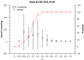
Figure 3 plots the distribution (mean and standard deviation) of the size of the /epsilon1 -coverings generated for problem class 〈 35 , 5 , 5 〉 , as a function of /epsilon1 . We can see that as /epsilon1 increases the size of the /epsilon1 -covering decreases considerably.

Impact of imprecise tradeoffs For the purpose of this evaluation, we generated consistent random tradeoffs between the objectives of a given problem instance, as follows. Let ( i, j ) be a pair of objectives picked randomly out of p objectives. We generate two tradeoffs a/vector e i -b/vector e j and b/vector e j -ac/vector e i , where /vector e i and /vector e j are the i -th and j -th unit vectors. Intuitively, one of the tradeoffs indicates how much of objective i one is willing to sacrifice to gain a unit of objective j , and the other is vice versa. In addition, we also generate a 3-way tradeoff between three objectives ( i, j, k ) picked randomly as well in the form of the tradeoff vector a/vector e i + b/vector e j -c/vector e k . Therefore, our random tradeoffs generator is characterized by parameters ( K,T,a,b,c ) , where K is the number of pairs of objectives, T is the number of triplets (and thus a total of 2 K + T tradeoffs in Θ ), and randomly chosen a, b, c ∈ [0 , 1) are used to construct the tradeoff vectors. Notice that parameter c can be used to control the strength of the two-way tradeoffs. Specifically,

Table 2: Results comparing algorithms ELIM-MOID and ELIM-MOID-TOF on random influence diagrams with random tradeoffs. Time limit 20 minutes.

size	w ∗		ELIM-MOID				ELIM-MOID-TOF
(C,D,O)		#	time	avg	stdev	med	#	time avg stdev			med
K = 1 ; T = 0 ; a, b, c ∈ [0 . 1 , 1)
(15,5,2)	9	9	139.58	2,714	2,864	1,673	94	24.93	98	232	1
(25,5,2)	11	7	18.25	2,344	2,614	269	92	7.12	33	126	1
(35,5,2)	14	2	283.29	9,115	8,934	9,024	83	59.18	147	378	1
(45,5,2)	16	2	397.72	7,596	7,536	7,566	76	23.08	86	302	1
(55,5,2)	18	4	717.68	10,422	5,851	14,896	76	48.02	90	233	2
K = 2 ; T = 1 ; a, b, c ∈ [0 . 1 , 1)
(15,5,3)	9	6	10.69	4,889	4,069	5,830	85	34.62	48	135	2
(25,5,3)	11	2	4.42	4,000	3,938	3,969	70	18.20	41	95	2
(35,5,3)	14	0					50	89.51	119	198	13
(45,5,3)	16	2	242.68	15,431	1,729	8,580	52	28.18	41	73	4
(55,5,3)	18	0					51	94.63	75	154	4
K = 6 ; T = 3 ; a, b, c ∈ [0 . 1 , 1)
(15,5,5)	9	3	65.73	15,062	12,229	14,741	84	19.70	41	104	4
(25,5,5)	11	1	50.35	21,074	0	21,074	74	83.30	97	217	4
(35,5,5)	14	0					59	63.69	101	225	8
(45,5,5)	16	0					61	96.59	107	216	8
(55,5,5)	18	0					41	84.32	51	101	12
K = 1 ; T = 0 ; a, b, c ∈ [0 . 1 , 1)
(15,10,2)	12	5	91.82	6,856	8,280	3,175	78	34.09	60	145	1
(25,10,2)	17	1	808.94	4,964	0	4,964	37	94.08	63	232	1
(35,10,2)	20	0					23	227.78	29	68	1
(45,10,2)	22	0					11	59.97	30	39	13
(55,10,2)	26	0					0
K = 2 ; T = 1 ; a, b, c ∈ [0 . 1 , 1)
(15,10,3)	12	0					45	157.48	86	191	12
(25,10,3)	17	0					11	204.78	74	83	73
(35,10,3)	20	0					3	303.42	8	8	4
(45,10,3)	22	0					3	158.17	4	4	1
(55,10,3)	26	0					0
K = 6 ; T = 3 ; a, b, c ∈ [0 . 1 , 1)
(15,10,5)	12	0					40	106.50	27	64	5
(25,10,5)	17	0					21	104.70	67	114	10
(35,10,5)	20	0					5	244.45	72	80	48
(45,10,5)	22	0					0
(55,10,5)	26	0					0

if we were to set c = 1 then the two objectives i and j would essentially collapse into a single one (we'd have precise rates of exchange between objectives i and j ). If c = 0 then the second tradeoff for the pair ( i, j ) is irrelevant.

Table 3: Impact of the quality of the random tradeoffs on bi-objective influence diagrams. Time limit 20 minutes.

size (C,D,O)	w ∗	ELIM-MOID					ELIM-MOID-TOF
		#	time	avg	stdev	med	#	time	avg	stdev	med
		K = 0 ;					K = 1 ; c = 0
(15,5,2)	9	9	139.58	2,714	2,864	1,673	84	48.30	243	542	23
(25,5,2)	11	7	18.25	2,344	2,614	269	61	16.83	79	260	10
(35,5,2)	14	2	283.29	9,115	8,934	9,024	42	94.89	190	344	11
(45,5,2)	16	2	397.72	7,596	7,536	7,566	42	76.83	130	297	5
(55,5,2)	18	4	717.68	10,422	5,851	14,896	41	144.64	268	312	78

Table 2 reports the results obtained with algorithms ELIMMOID and ELIM-MOID-TOF, respectively. For each problem class 〈 C, D, O 〉 we generated 10 random instances, and for each problem instance we generated 10 sets of random tradeoff vectors using the parameters K,T,a,b,c indicated in the header of each horizontal block. As before, the columns labeled by # show how many problems out of 10 (respectively, out of 100) were solved by ELIM-MOID (respectively, ELIM-MOID-TOF). Overall, we notice that the expected utility sets computed by ELIM-MOID-TOF are orders of magnitude smaller than the corresponding Pareto optimal ones generated by ELIM-MOID. We also see that the median size is even smaller, in some cases being ac-

tually 1 indicating that the tradeoffs generated were strong enough to make /followsequal Θ fairly close to being a total order.

In Table 3 we take a closer look at the impact of the tradeoffs strength for bi-objective problems with 5 decisions. We see that even exploiting a single tradeoff (i.e., using c = 0 for two objective case) has a dramatic impact on the size of the maximal expected utility set. For example, on problem class 〈 55 , 5 , 2 〉 , the undominated set of expected utility values computed by ELIM-MOID-TOF contains on average 38 times fewer utility values than the corresponding Pareto optimal set generated by ELIM-MOID.

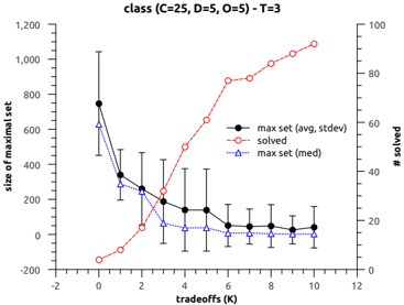
Figure 4 shows the distribution (mean, standard deviation and median) of the size of the maximal sets generated by ELIM-MOID-TOF on problems from class 〈 25 , 5 , 5 〉 as a function of the number of pairwise tradeoffs K . As more tradeoffs become available the number of problem instances solved increases because the /followsequal Θ -dominance gets stronger and therefore it reduces the undominated utility sets significantly.

7 CONCLUSION

In this paper, we describe how a variable elimination solution method for influence diagrams is extended to the case of multi-objective utility. A general problem with using the Pareto ordering for multi-objective utility is that the set of maximal expected utility values will often become extremely large. We show how the use of /epsilon1 -coverings can lead to a much more practical computational approach than the exact computation.

We also define a natural way of taking imprecise tradeoffs into account, and give a computational method for checking the resulting dominance condition. Our experimental results indicate that the resulting maximal (multi-objective) values of expected utility can be very much reduced by the adding of (even a small number of) tradeoffs.

References

1. R. Howard and J. Matheson. Influence diagrams. In Readings on the Principles and Applications of Decision Analyis , pages 721-762, 1984.
2. R. Keeney and H. Raiffa. Decisions with multiple objectives: preferences and value tradeoffs . Cambridge University Press, 1993.
3. B. Roy. Multicriteria methodology for decision analysis . Kluwer Academic Press, 1996.
4. M. Ehrgott. Multicriteria optimization . Springer, 1999.
5. N. Wilson and R. Marinescu. An axiomatic framework for influence diagram computation with partially ordered utilities. In International Conference on Principles of Knowledge Representation and Reasoning (KR) , pages 210-220, 2012.
6. M. Diehl and Y. Haimes. Influence diagrams with multiple objectives and tradeoff analysis. IEEE Transactions On Systems, Man, and Cybernetics Part A , 34(3):293-304, 2004.
7. R. Shachter. Evaluating influence diagrams. Operations Research , 34(6):871-882, 1986.
8. C. Papadimitriou and M. Yannakakis. On the approximability of trade-offs and optimal access to web sources. In IEEE Symposium on Foundations of Computer Science (FOCS) , pages 86-92, 2000.
9. J-P. Dubus, C. Gonzales, and P. Perny. Multiobjective optimization using GAI models. In International Joint Conference on Artificial Intelligence (IJCAI) , pages 1902-1907, 2009.
10. L. Zhou, W. Liu, and L. Wang. Influence diagram model with interval-valued utilities. In IEEE International Conference on Dependable, Autonomic and Secure Computing (DASC) , pages 601-605, 2009.
11. G. Cooper. A method for using belief networks as influence diagrams. In Uncertainty in Artificial Intelligence (UAI) , pages 9-16, 1988.
12. D. Kikuti and F. Cozman. Influence diagrams with partially ordered preferences. In Proceedings of 3rd Multidisciplinary Workshop on Advances in Preference Handling , 2007.
13. D. Kikuti, F. Cozman, and R. Filho. Sequential decision making with partially ordered preferences. Artificial Intelligence , 175(7-8):1346-1365, 2011.
14. C. de Campos and Q. Ji. Strategy selection in influence diagrams using imprecise probabilities. In Uncertainty in Artificial Intelligence (UAI) , pages 121128, 2008.
15. M. L´ opez-D´ ıaz and L. Rodr´ ıguez-Mu˜ niz. Influence diagrams with super value nodes involving imprecise information. European Journal of Operational Research , 179(1):203-219, 2007.
16. D. Maua and C. de Campos. Solving decision problems with limited information. In Advances in Neural Information Processing Systems (NIPS) , pages 603611, 2011.
17. P. Yu. Cone convexity, cone extreme points, and nondominated solutions in decision problems with multiobjectives. Journal of Optimization Theory and Applications , 14(3):319-377, 1974.
18. M. Wiecek. Advances in cone-based preference modeling for decision making with multiple criteria. Decision Making in Manufacturing and Services , 1(12):153-173, 2007.
19. J. Pearl. Probabilistic Reasoning in Intelligent Systems . Morgan Kaufmann, 1988.
20. F. Jensen, V. Jensen, and S. Dittmer. From influence diagrams to junction trees. In Uncertainty in Artificial Intelligence (UAI) , pages 367-363, 1994.
21. H. Raiffa. Decision analysis . Addison-Wesley, 1968.
22. J. Tatman and R. Shachter. Dynamic programming and influence diagrams. IEEE Transactions on Systems, Man, and Cybernetics , 20(1):365-379, 1990.
23. P. Shenoy. Valuation-based systems for Bayesian decision analysis. Operations Research , 40(1):463-484, 1992.
24. R. Dechter. A new perspective on algorithms for optimizing policies under uncertainty. In Artificial Intelligence Planning Systems (AIPS) , pages 72-81, 2000.
25. C. Pralet, T. Schiex, and G. Verfaillie. Sequential decision making problems - representation and solution . Wiley, 2009.
26. C. Gonzales, P. Perny, and J-P. Dubus. Decision making with multiple objectives using GAI networks. Artificial Intelligence , 175(1):1153-1179, 2011.
27. Y. Zheng and C. Chew. Distance between a point and a convex cone in n-dimensional space: computation and applications. IEEE Transactions on Robotics , 25(6):1397-1412, 2009.