On the Use of Skeletons when Learning in Bayesian Networks

Harald Steck*

Siemens AG, Corporate Technology Neural Computation Dept. Information and Communications

Otto-Hahn-Ring 6, 81730 Munich, Germany

Abstract

In this paper, we present a heuristic operator which aims at simultaneously optimizing the orientations of all the edges in an interme­ diate Bayesian network structure during the search process. This is done by alternating between the space of directed acyclic graphs (DAGs) and the space of skeletons. The found orientations of the edges are based on a scoring function rather than on induced con­ ditional independences. This operator can be used as an extension to commonly employed search strategies. It is evaluated in experi­ ments with artificial and real-world data.

1 INTRODUCTION

Much progress has been made regarding structural learning in Bayesian networks. In the course of which, two main approaches have evolved. The one is constraint-based and relies on inducing conditional independences from the (empirical) probability distri­ bution over the variables in a domain, e.g. [16], and the other tries to optimize a scoring function by means of a (heuristic) search strategy, e.g. [7, 9]. In the latter approach, scoring functions like the posterior proba­ bility or penalized likelihoods, e.g. the Bayesian Infor­ mation Criterion (BIC), might be used. Finding the optimum Bayesian network structure was shown to be an NP-complete problem [5], so that one has to resort to heuristic search strategies.

Several Bayesian network structures, which are dis­ played by directed acyclic graphs (DAGs), can be Markov equivalent. An equivalence class contains all those DAGs which represent the same probabil­ ity distributions determined by the conditional in­ dependences and dependences, see for instance [14].

also: Dept. of Computer Science, Technical University of Munich, 80290 Munich, Germany; [email protected]

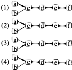
When learning from a probability distribution, score­ equivalent scoring functions are commonly used, i.e. the same score is assigned to Markov equivalent DAGs. As a consequence, this can prevent local search proce­ dures from finding optimum DAGs. For instance ( cf. Fig. 1), assume that a local search procedure has ar­ rived at the intermediate DAG (1). Let us further assume that the optimum DAG comprising the same edges is the one as depicted in (4). The DAGs (1), (2) and (3) are equivalent. Hence, only in the transition from DAG (3) to (4), there is a difference regarding the scores assigned to the DAGs. If exhaustive search is infeasible, the transitions from DAG (1) to DAG (3) via DAG (2) might not be found by a simple lo­ cal search procedure, because these transitions are not related to an improvement regarding the score.

In order to get around this problem due to Markov equivalent DAGs, it has been proposed and examined to carry out local search in the space of equivalence classes rather than in the space of DAGs, which has several advantages, see for instance [12, 6]. A disad­ vantage is, however, that the number of neighboring graphs in the space of equivalence classes can be much larger than in the space of DAGs. Also, determining neighboring equivalence classes given an intermediate one can be computationally quite costly. Since this can

render such an approach rather involved, it was pro­ posed to alternate between the search space of DAGs and the space of equivalence classes for efficient com­ putation (6].

In this paper, we present a heuristic search operator which makes use of skeletons. A skeleton is the graph obtained by substituting each directed edge in a DAG by an undirected one. The operator comprises two steps: Given an intermediate DAG in the search pro­ cess, it is first transformed to its corresponding skele­ ton. In the second step, the proposed operator aims at orienting the edges in such a way that the result­ ing DAG is optimum (among the DAGs with the same skeleton) with respect to the used scoring function. In this paper, we focus on finding a single (optimum) graph as opposed to inducing several DAGs like it is done for model averaging, e.g. (17]. Since an equiv­ alence class of DAGs is defined by its skeleton and the colliders ( v-structures) (18], the heuristic search operator first identifies the colliders before orienting the remaining edges. This is similar to the constraint­ based procedures used in the SGS or PC algorithms (16]. The main difference is that the presented op­ erator orients the edges according to the used scoring function rather than according to the conditional inde­ pendences and dependences induced from the ( empir­ ical) probability distribution. This rendered the pre­ sented operator quite robust in our computer experi­ ments, whereas the edge-orientation procedures used in the SGS or PC algorithms are known to be rather unstable when applied to finite samples (16].

In the above simplistic example ( cf. Fig. 1 ), the pre­ sented search operator yields the transition from the intermediate DAG (1) to the optimum DAG (4) at once without being affected by the equivalent DAGs (2) and (3). This is because it alternates from the DAG (1) to its skeleton, and then orients all edges again: First, the collider at the node c is identified, which determines the equivalence class. Then the edges be­ tween c and d, between d and e, and between e and f are oriented such that no additional colliders oc­ cur. Alternating between the search space of DAGs and the space of skeletons might thus serve as an inex­ pensive alternative to using the search space of equiv­ alence classes. The operator presented in this paper can help search strategies in the space of DAGs get out of local maxima, and might thus be used as an extension to commonly employed constraint-based ap­ proaches as well as to many greedy search strategies like local search.

Having applied this operator to an intermediate DAG during the search process, the orientations of several edges might be changed compared to the previous DAG. This is in contrast to local search, where subse- quent DAGs differ from each other by exactly one di­ rected edge, which is included, eliminated or reversed. The presented operator might thus be considered as non-local.

This paper is organized as follows. First, we are con­ cerned with decomposable scoring functions, which are an essential requirement of the presented operator. For ease of computation, we approximate the poste­ rior probability by employing the Bayesian Informa­ tion Criterion (BIC). The next section provides the details of the operator: It focuses on the scoring func­ tion used for orienting the colliders ( v-structures) and on the procedures for subsequently orienting the re­ maining edges. Finally, in our computer experiments, we used the operator as part of a very simple search strategy in order to compare the beneficial effects due to the presented operator to other search strategies like the K2 algorithm [7] or the local search strategy applied to learning in Bayesian networks [9].

2 DECOMPOSABLE SCORE

In this paper, we assume the scoring function to be decomposable, i.e. to factorize recursively like the joint probability distribution over the set of variables V = { x1, .. . , Xn } described by a Bayesian network,

where pam(x;) denotes the parents of the node 1 x; in the DAG m. Commonly used scoring functions factor­ ize in this fashion in the case of complete data and in the absence of latent variables. As a particular choice for the scoring function, we use the posterior probabil­ ity

of the DAG m when given data D. Simplifying the computation for practical reasons, we approximate the marginal likelihood p(Dim) by the Bayesian Informa­ tion Criterion (BIC),

The BIC states the trade-off between the maximum likelihood L( B) of the model and its dimension I BI in an intuitive way. Unlike the Akaike criterion, the term penalizing model complexity depends on the number N of cases in the given sample. The BIC is a rough approximation, and it avoids the introduction of priors over the parameters. For more details, the reader is referred to [11].

1 For simplicity, we use node and variable synonymously.

First of all, let us consider two nested DAGs which differ from each other by exactly one edge. Let the corresponding two DAGs be denoted by m1 and mz, where the DAG m1 contains one edge more than mz, and let this additional edge in m 1 be oriented from node a E V to node b E V \ {a}, indicated by a -t b. For brevity, we denote the parents of node b in the sparser graph mz by 1r = p a m2 ( b ).

In order to compare the two DAGs m1 and mz it is a natural choice to use posterior odds. With the above approximation, one arrives at the relative scoring func­ tion G which gives the score of m1 relative to mz:

This score was used for model selection in [3], where the maximum a posteriori rather than the maximum likelihood configuration of the parameters was chosen. Assuming discrete variables with a multinomial distri­ bution, the maximum likelihood ratio is given by

where the sum is over all configurations of a, b and 1r. The counts from the data are denoted by Na,b,rr, where the "+" indicates that it is summed over the corresponding variable(s). Since the DAGs m1 and m2 differ in exactly one edge, the likelihood ratio depends only on the involved variables a, b, and 1r, and it is independent of the remaining ones. This holds also for the degrees of freedom dr,

where the number of (joint) states of a (set of) van­ able(s) is denoted by S. Instead of Eq. 5, one might use adjusted degrees of freedom [ 2].

In order to attain a prior p(m) which decomposes in the same fashion, one may resort, for instance, to the assignment p(m) ex: exp(al£(m)l) with the number of edges l£(m)l in the DAG m and with a constant a for a priori penalizing DAGs dependent on the number of edges. Then the function G depends only on the variables a, b and 1r. It is score-equivalent [4).

If one is interested in a notably higher score of m1 compared to mz one may use a threshold value 1 > 0 in G(a, b, 1r ) 2: /, see for instance [11].

3 DETAILS OF THE OPERATOR

This section provides the details of the proposed search operator which alternates between the search space of

DAGs and the space of skeletons. In the first step, the current DAG is transformed to its skeleton, which is simply done by dropping the directions of the edges. Given a skeleton in the second step, the aim is to find the orientations such that the resulting DAG corre­ sponds to the maximum of the scoring function. Of course, this problem can only be tackled in a limited way. For simplicity, we use a greedy scheme, i.e. at an intermediate step of the edge-orientation process we orient the edge which increases the score most.

3.1 ORIENTING COLLIDERS

In this step, we use a partially directed acyclic graph (PDAG) which contains the same edges as the given skeleton. Initially, all its edges are undirected, at an intermediate stage some edge are oriented, and even­ tually all the edges of the PDAG are directed. In the PDAG, a structure which is a candidate for being a collider involves three nodes a, band c such that there is an edge between a and b as well as between b and c; there is no edge between a and c. We denote an undi­ rected edge between two variables x and y by x "' y, an oriented one by x =? y, and an edge with a proposed orientation by x -t y ( cf. Algo. 1).

In an intermediate PDAG mint, it has to hold for a collider candidate that a '--+ b t---' c with +--'E { "' , {:::} and '-+E { "' , =} }. This means that the edges are not allowed to be already oriented like a {::: b or b * c. For each of the collider candidates the score Gcol is calculated as described in the following section. Next, the collider candidate with the largest score Gcot(a,b,c I Tnint ) 2: 1 is oriented like a =} b {::: c. After a collider has been oriented, one has to make sure that there cannot occur a (directed) cycle in the PDAG when orienting one more edge. Such edges are thus oriented in the opposite direction without con­ sidering the scoring function for simplicity. After a collider or an edge have been oriented in the PDAG Tnint, some of the scores Gcol (a, b, c I Tnint ) have to be updated. The above steps are repeated while there are collider candidates with a score larger than I·

3.2 SCORING COLLIDER CANDIDATES

Given an intermediate PDAG Tnint, the score Gcot(a,b,c I Tnint ) of a collider candidate a'--+ b t---' c is calculated by comparing DAGs with each other which are identical except of the orientations of the edges a '--+ b and b t---' c. In particular, the variables a, b and c have the same parents as in the PDAG mint, i.e. pa m;no (a), pa mint (b), and pa mint (c), respectively. Let us denote the DAG with the collider a =} b {::: c by me and the three alternative DAGs (without that collider) by

• m._ with the two edges oriented as a -¢= b -¢= c,
• m--+ with the two edges oriented as a =} b =} c,
• m+-+ with the two edges oriented as a {= b =}c.

Like in Sec. 2, we use the approximation of the posterior odds in order to score the DAG me rela­ tive to the alternative DAG m._ by the relative score G._(a,b,c I mint),

where we have used the scoring function G as denoted in Eq. 4. The second line indicates a considerable sim­ plification since the scoring function is decomposable. Analogously, one arrives at the scores of me relative to m--+, i.e. G--t(a,b,c I mint), and relative to m+-+, i.e. Gt-t(a,b,c I m in t ),

For reasons regarding the stability of the algorithm we use the following score of a collider candidate:

If Gcot(a,b,c I m int) > 0, this score is a lower bound for the increase of the overall score of the graph which comprises a collider compared to an alternative graph which is identical with me except of this collider. If Gcot(a,b,c I mint)< 0, this is a bound for the max­ imum decrease of the score when these edges are ori­ ented as a collider compared to one of the alternative orientations.

3.3 ORIENTING REMAINING EDGES

After the colliders have been oriented, the algorithm orients the remaining edges as follows. Guided by the heuristic of parsimony the aim is to find an orientation of the remaining edges such that a minimum number of additional colliders occurs. In the ideal case, where a perfect map of the probability distribution over the variables exists, this is possible without introducing an additional collider. In this case, the procedure ProposeOrientations ( cf. Algo. 1) indicates the ori­ entations of the remaining edges by arrows of the type -+or t-, and no arrows of the type t-t are found; edges whose orientations can differ in equivalent DAGs are indicated by "', and they are oriented in the final step.

• procedure ProposeOrientations input: PDAG mint with edges "' , =}, -¢=. output: PDAG mint with edges "' , =}, -¢=, -+, f-, t-t. (1) Va , b , c E V: if a'---+ b t-' c with <---+E {=}, -+ , t-t} and f-'E { "', f-} and no edge between a and c then substitute either b rv c by b -+ or b fc by b t-t c. (2) Va, b E V: while 3 a fb and 3 a = x1, ... ,xq = b (xi=/=- X j ,q > 2) such that Xi-1 '---+Xi (i = 2, .. . ,q) with <---+E {=}, -+, t-t} then substitute a fb by a t-t b. (3) while edges can be oriented go to (1).

Algorithm 1: The procedure ProposeOrzentations tries to orient the edges in such a way that no addi­ tional colliders occur. If this is not possible, edges are oriented in "both" directions, indicated by t-t.

procedure FixOrientations input:

PDAG mint, data D

output:

PDAG mint

1. call ProposeOrientations.
2. substitute uniquely oriented edges a -+ b by a =} b.
3. ( 3) among all structures of the form a t-t b t-t c without an edge between a and c, orient the one with the highest score Gcot (a, b, c l m ; n t ) like a =} b {=c.
4. ( 4) if there are edges of the type t-t then substitute all those by "' and go to ( 1).

Algorithm 2: This procedure resolves inconsisten­ cies regarding the orientations of edges (indicated by t-t) by using the scoring function.

In step (2) of the procedure Fix Orientations ( cf. Algo. 2), the orientations of those edges are fixed (by a double-arrow=} or{=) whose orientations are uniquely indicated by the procedure Pr-oposeOrientations (de­ noted by f- or -+). However, if an edge of the type t-t is proposed by the procedure ProposeOrientations, the edges cannot be oriented such that no additional colliders occur. Hence, in step (3) of the procedure Fix Orientations, we propose to orient the pair of am­ biguously oriented edges like a collider which gets the

highest score. Note that the score Gcol might be neg­ ative in this case. Hence, orienting the highest scoring edges like a collider corresponds to decreasing the over­ all score as little as possible in this greedy scheme.

Like the procedure ProposeOrientations, also FixOrientations has to make sure that a (directed) cycle cannot occur when fixing the orientations of the edges. Hence, the step ( * ) has to be carried out each time an edge has been oriented like {=: or ::::} by the procedure Fix Orientations. Note that ( * ) focuses on possible cycles due to edges whose orientations are al­ ready fixed.

After FixOrientations is finished, there might still be undirected edges in the PDAG, as already mentioned. Those edges are oriented in a final step of the edge­ orientation procedure. This is done by randomly pick­ ing one of those edges and by assigning to it a random orientation. Then the procedure FixOrientations is called in order to orient the edges which are affected by this assignment. This is repeated until all edges are oriented.

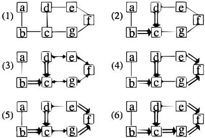
For illustration, let us consider the example in Fig. 2: Assume that the only collider with a score Gcol 2: 1 is b ::::} c {=: d, cf. (2). When orienting the remain­ ing edges, Propose Orientations indicates inconsisten­ cies ( f+) due to a possible directed cycle, cf. (3). Hence, an additional collider is introduced, namely the one with the highest score Gcol < /, e.g. at the node J, see (4). In subsequent steps, no inconsistencies oc­ cur, so that the orientation of the edge between c and gand hence the equivalence class- can be identified, cf. (5) and (6).

�D

Figure 2: A simplistic example how the procedures ProposeOrientations and FixOrientations work.

3.4 STABILITY

The presented procedure for orienting the edges given a skeleton is similar to the ones used in the SGS and PC algorithms [16]. The main difference is that our procedure aims at finding the orientations such that a scoring function is maximized. Of course, since a greedy approach is taken, this procedure might only find a local optimum. In contrast, the SGS and PC algorithms orient the edges based solely on the con­ ditional independences induced from the data. This is correct, if the probability distribution is perfectly known and if there exists a perfect map [16). Given finite data, however, the latter procedures are known to be unstable (cf. [16]), whereas we found the pre­ sented procedure to be quite stable in our computer experiments.

3.5 LIMITATIONS OF THE HEURISTIC

Finding the skeleton corresponding to a given DAG is straight-forward. In contrast, the second step of the presented operator is, of course, not guaranteed to find the global optimum regarding the orientations of the edges, since learning Bayesian networks is an NP­ complete problem [5]. However, it might serve as an efficient way of finding close to optimum orientations.

The heuristic operator calculates the score of the col­ lider candidates based on the edges which have already been oriented in the intermediate graph. Of course, this can only be an approximation to the "correct" scores. In particular, at the beginning of this proce­ dure, when only a small number of edges has already been oriented, the computed scores might considerably differ from the "correct" scores, because the optimum parents might not be known at this stage. Hence, this greedy procedure might get stuck at a local optimum. When orienting the remaining edges, there might oc­ cur inconsistencies regarding the directions, which in­ dicate that additional colliders have to be introduced in order to attain a DAG. This is done in a heuris­ tic way by orienting those edges like a collider which entail the smallest decrease regarding the score. Addi­ tionally, it has to be made sure that no directed cycles arise during this procedure. This is done in a simple heuristic way without considering the score. For an evaluation of the presented heuristic operator one has to resort to computer experiments.

4 PRELIMINARY EXPERIMENTS

In our computer experiments, we used the pre­ sented operator together with two additional opera­ tors, namely one for forward inclusion and one for backward elimination, in order to arrive at a simple search strategy, which we call skeleton search strategy in the remainder of this section. We compared this search strategy with other ones like the K2 algorithm [7] and the greedy algorithm based on local search, as described for instance in [9). In detail, this sim­ ple search strategy works as follows: Starting out with

the empty DAG, the graph is optimized by repeatedly cycling through the following three steps:

1. apply the presented operator
2. carry out one step of forward inclusion m the space of DAGs
3. perform backward elimination m the space of DAGs

After the orientations of the edges have been optimized by the presented operator, the edge which improves the score most is included into the DAG. Of course, no (directed) cycles may occur in the resulting graph. In this scheme, at most one edge is included into the graph in each cycle of the algorithm so that the pre­ sented operator can optimize the orientations before the next edge is included. The third step allows the algorithm to remove edges which have been included previously when the orientations of some edges might have been different. It might occur that this simple search strategy oscillates among two or more DAGs at the end of the search process, i.e. it may not converge to a unique DAG. This is because the presented oper­ ator is non-local in the sense that it possibly changes the orientations of more than one edge. For the stop­ ping criterion this has to be taken into account, and we propose to keep track of the last few DAGs and to eventually choose the one with the highest score.

The results in our computer experiments were ob­ tained from the following real-world data sets: The data (SEW) was gathered by Sewell and Shah [15], and it is concerned with high-school students. It com­ prises 5 variables and over 10,000 cases. The data (ENV) is concerned with environmental influences on the condition of trees [10]. It contains 11 variables and 6168 cases. In our experiments, we ignored the first and the ninth variable of this data set, since the latter is not documented and the former has several hundred states which encode the position of the trees with respect to a grid on a map. Moreover, we dis­ cretized the last two variables in this data set such that each variable had four states. We obtained the data (BOS) by discretizing the variables of the Boston Housing Data [8] such that each variable became bi­ nary. This sample contains 14 variables and 506 cases. The data (CAR) contains 46 variables, and 794 cases were available from [13]. It was gathered from cus­ tomers of a car company. The two variables VORMD and URTEI have 16 and 10 states, respectively. For practical reasons, we summarized some of their states such that these two variables had 3 and 4 states, re­ spectively.

When comparing the different search strategies we ap­ plied the same scoring function G ( cf. Eq. 4) to each of the strategies. We committed ourselves to a uni­ form prior over the DAGs, p( m) = const, and imposed no constraints on the network structures. The thresh­ old value 1/2 = 3 was used in order to include only those edges into the graph which lead to some notable increase in the score [11]. The parameters Om of an induced DAG m were calculated in a Bayesian way, namely as the expectation values of the posterior dis­ tributions over the parameters. We used conjugate priors and a small equivalent sample size of N' = 5, see for instance [9].

Table 1: Experiments with four real-world data sets. The results are assessed by 5-fold cross validation (XV), cf. Sec. 4 for details.

data set	nodes	skeleton search XV	local search XV
SEW	5	0.0504 ± 0.0035	0.0514 ± 0.0034
ENV	11	0.877 ± 0.018	0.921 ± 0.040
BOS	14	1.94 ± 0.11	2.15 ± 0.12
CAR	46	25.53 ± 0.26	25.54 ± 0.26

In order to assess the expected utility of the Bayesian networks induced by the different search strategies we carried out 5-fold cross validation (XV), cf. [9]. The Kullback-Leibler divergence was used in order to com­ pare the probability distributions underlying the val­ idation sets with the ones described by the induced Bayesian networks. In Table 1, we depicted the mean and the standard deviation of the Kullback-Leibler di­ vergence when averaged over the 5 samples in cross validation. Small values indicate good learning re­ sults. We compared the skeleton search strategy to the greedy algorithm based on local search as described, for instance, in [9].

Considering cross validation, the skeleton search strat­ egy yields slightly better DAGs than does local search for each of the data sets in Table 1. The differences might be considered notable regarding the data sets (ENV) and (BOS), because the difference in the means is not considerably smaller than the standard devia­ tions. This does not hold for the data sets (SEW) and (CAR). Considering the used scoring function BIG in the experiment with the data (SEW), the simple skele­ ton search strategy found the global optimum, whereas local search found only a local optimum. The large val­ ues concerning the tiny data set (CAR) might indicate that this data set cannot be well described by means of a Bayesian network model.

In our Alarm network [1] experiments, we used the posterior probability with conjugate priors as the scor­ ing function, see for instance [9]. The learning algo­ rithms employed the corresponding relative score G

which can be derived for the posterior probability with conjugate priors analogously to Eq. 4. A small value of the equivalent sample size was chosen, i.e. N' = 1. We note that the Kullback-Leibler divergence computed in cross validation did not very sensitively depend on the chosen equivalent sample size which we varied between N' = 1 and N' = 100. This was also noted in [9]. Re­ garding the number of edges in the induced graph, we observed their number to increase when the equivalent sample size N' rises.

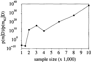
In order to examine the stability of the presented oper­ ator concerning different sample sizes, we applied the skeleton search strategy to data sets of various sizes sampled from the probability distribution described by the Alarm network [1]. The Alarm network con­ tains 37 discrete variables and 46 edges. Since the (partial) ordering of the variables is known, we could use the K2 search strategy [7] for comparison. The K2 procedure requires an initially specified ordering of the variables, and one can, hence, expect this search strategy to be quite stable regarding different sam­ ple sizes. In Fig. 3, we compare the skeleton search strategy to the K2 search strategy. Given only small samples (with less than 2,000 cases), our search strat­ egy gets stuck at a local optimum which is far from the global one. The prior knowledge about the cor­ rect ordering of the variables seems to be crucial for the K2 procedure in the case of small samples. How­ ever, from samples containing at least 2, 000 cases, the skeleton search strategy induces DAGs which get a higher score than the ones found by the K2 search strategy. Considering structural differences, we no­ ticed that the K2 algorithm tends to include slightly more edges into the graph than the skeleton search strategy does. Compared with the original Alarm net­ work structure, one edge was usually "erroneously" removed by both search strategies in most of our ex­ periments, since this was favored by the scoring func­ tion. Except of this, the skeleton search strategy either induced the correct structure or - in particular when given small data sets - got stuck at a local optimum which erroneously contained an additional edge which was related to a "wrong" orientation of another edge. The K2 algorithm usually included one, and sometimes two, edges "erroneously".

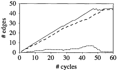
Finally, we examined how quickly the skeleton search strategy reaches the end of the search process, i.e. how many cycles it takes to identify an approximately op­ timum structure. Since in each cycle at most one edge is added, the number of cycles cannot be smaller than the number of edges present in the induced DAG. In our Alarm network experiments, we found that the number of edges being present in the graph increases quite quickly before the end of the search process is

60

reached ( cf. Fig. 4). Since information about the ordering of the variables is not given as input to our algorithm, edges are "erroneously" included into the graph. Towards the end of the search process, after the orientations of the edges have been established, most of the "erroneously" included edges are removed in this example. We found that the resulting DAG got a higher score than the one induced by the K2 search strategy, although the latter used the correct ordering of the variables as prior knowledge.

In our computer experiments, we observed that com­ puting the counts N of the different configurations of several variables is typically very time consuming. In fact, most of the computation time was spent on this task. Hence, a lot of computation time can be saved by caching the scores G once they have been computed. Since the DAGs in subsequent cycles are usually sim­ ilar to each other, this caching can lead to a large

speed-up.

5 CONCLUSIONS

In this paper, we presented a search operator which makes use of skeletons. In order to derive a DAG when given a skeleton, the edges are oriented with the aim of finding the optimum orientations with respect to a scoring function. This is in contrast to other proce­ dures of this kind, e.g. the ones used in the PC or SGS algorithms (16], which are based on induced con­ ditional independences, and which are known to be un­ stable when applied to finite data. Since the presented operator might simultaneously change the orientations of several edges it can be considered as non-local in the space of DAGs. The presented operator first iden­ tifies the colliders, which determine the equivalence class, and subsequently orients the remaining edges. This operator was thus quite robust against problems entailed by Markov-equivalent network-structures in our computer experiments. The operator was used in a simple search strategy which we compared to com­ monly used learning algorithms. Our preliminary ex­ periments with artificial and real-world data suggest that alternating between the search space of DAGs and the space of skeletons might serve as a powerful and computationally efficient alternative to more involved search strategies.

Acknowledgments

I would like to thank Steffen Lauritzen for his hospi­ tality and for numerous enlightening discussions. I am also grateful to Paul Theo Pilgram, Volker Tresp, and anonymous reviewers for valuable comments which helped improve this paper. This work was supported by an Ernst-von-Siemens grant.

References

• (1] I. A. Beinlich, H. J. Suermondt, R. M. Chavez, and G. F. Cooper. The Alarm Monitoring System: A Case Study with Two Probabilistic Inference Techniques for Belief Networks. In Proc. of the Second European Conf. on Artificial Intelligence in Medicine, pages 247-56. London, UK, 1989.
• (2] Y. Bishop, S. Fienberg, and P. Holland. Discrete Multivariate Analysis. MIT Press, 1975.
• (3] P. Cheeseman and J. Stutz. Bayesian Clas­ sification (AUTOCLASS): Theory and Results. In U. Fayyad, G. Piatesky-Shapiro, P. Smyth, and R. Uthurusamy, editors, Advances in Knowl­ edge Discovery and Data Mining, pages 153-180. AAAI Press, Menlo Park, CA, 1995.
• (4] D. M. Chickering. A Transformational Charac­ terization of Equivalent Network Structures. In Proc. of the Conf. on Uncertainty in Artificial In­ telligence, pages 87-98, 1995.
• (5] D. M. Chickering. Learning Bayesian Networks is NP-Complete. In Proc. of AI 3 STAT, pages 121-30, 1996.
• (6] D. M. Chickering. Learning Equivalence Classes of Bayesian Network Structures. In Proc. of the Conf. on Uncertainty in Artificial Intelligence, pages 150-7, 1996.
• (7] G. Cooper and E. Herskovits. A Bayesian Method for the Induction of Probabilistic Networks from Data. Machine Learning, 9:309-47, 1992.
• (8] Boston Housing Data. see for instance StatLib Datasets Archive, http:/ /lib.stat.cmu.edu/ datasets/boston.
• (9] D. Heckerman, D. Geiger, and D. M. Chickering. Learning Bayesian Networks: The Combination of Knowledge and Statistical Data. Technical re­ port, MSR-TR-94-09, Microsoft Research, 1994.
• (10] Environmental Influences on the Condition of Trees. Data Sets at the Dept. of Statistics, Univ. of Munich, http:/ /www.stat.uni-muenchen.de/ data-sets/fioss/floss.html.
• (11] R. E. Kass and A. E. Raftery. Bayes Factors. JASA, 90:773-96, 1995.
• (12] D. Madigan, S. A. Andersson, M. D. Perlman, and C. T. Volinsky. Bayesian Model Averag­ ing and Model Selection for Markov Equivalence Classes of Acyclic Digraphs. Communications in Statistics Theory and Methods, 25(11):2493519, 1996.
• (13] Consumer-Satisfaction of Car Owners. Data Sets at the Dept. of Statistics, Univ. of Munich, http:/ /www.stat.uni-muenchen.de/data-sets/ bmw /bmw.html.
• (14] J. Pearl. Probabilistic Reasoning in Intelligent Systems. Morgan Kaufmann, 1988.
• (15] W. Sewell and V. Shah. Social Class, Parental En­ couragement, and Educational Aspirations. Am. J. of Sociology, 73:559-572, 1968.
• (16] P. Spirtes, C. Glymour, and R. Scheines. Cau­ sation, Prediction, and Search. Springer Lecture Notes in Statistics 81, 1993.
• (17] B. Thiesson, C. Meek, D.M. Chickering, and D. Heckerman. Learning Mixtures of DAG Mod­ els. In Proc. of the Conf. on Uncertainty in Arti­ ficial Intelligence, pages 504-13, 1998.
• (18] T. Verma and J. Pearl. Equivalence and Synthesis of Causal Models. In Proc. of the Conf. on Un­ certainty in Artificial Intelligence, pages 220-227, 1990.