On Transformations between Probability and Spohnian Disbelief Functions

Phan H. Giang and Prakash P. Shenoy

erfield Hall

University of Kansas School of Business, S umm Lawrence, KS 66045-2003, USA pgiang@ukans. edu, pshenoy@ukans. edu

Abstract

In this paper, we analyze the relationship b& tween probability and Spohn's theory for rep­ resentation of uncertain beliefs. Using the in­ tuitive idea that the more probable a propo­ sition is, the more believable it is, we study transformations from probability to Spoh­ nian disbelief and vice-versa. The transfor­ mations described in this paper are different from those described in the literature. In particular, the former satisfies the principles of ordinal congruence while the latter does not. Such transformations between proba­ bility and Spohn's calculi can contribute to ( 1) a clarification of the semantics of non­ probabilistic degree of uncertain belief, and (2) to a construction of a decision theory for such calculi. In practice, the transformations will allow a meaningful combination of more than one calculus in different stages of using an expert system such as knowledge acquisi­ tion, inference, and interpretation of results.

1 Introduction

In [19, 20] Spohn describes a non-probabilistic theory for epistemic belief representation. One notable ad­ vantage of this theory compared to probability theory is in representing the notion of plain belief that is sup­ posed to be deductively closed. The deficiency of prob­ ability theory to do such a job has been demonstrated by the well-known Lottery Paradox that describes the situation in which each of a million lottery players has no practical chance to win the jackpot, nevertheless, one among them will surely win. Another nice feature of Spohn's theory is its naturally defined concept of conditionals which is similar to its probabilistic coun­ terpart in many aspects. Hunter [9] and Shenoy [13] exploit that structural similarity to implement Spohn's theory using computational architectures traditionally used for probability such as valuation networks and Bayesian networks. From a theoretical perspective, on one hand, Dubois and Prade [4] observe that the basic representation in Spohn's theory, the disbelief function, can be interpreted as the negative of the log­ arithm of a possibility function. On the other hand, interpretation of disbelief values as infinitesimal proba­ bilities makes Spohn's theory tightly related to Adams' study of E-semantics for default reasoning [1]. Thus, Spohn's theory is well positioned in the web of quan­ titative approaches to represent and reason about un­ certain beliefs. In the remainder of this section, we shall briefly review the theory and ask questions that motivate the study of Spohn's belief-probability trans­ formations.

Let n denote a set of possible worlds. For simplicity, we assume n is finite , 1!21 = n. We use w (perhaps with subscripts) to denote a world, i.e. w E !2.

A Spohnian disbelief function {j is defined as a mapping

where z+ is set of non-negative integers. {j satisfies the following axiom:

An extension of {j to the set of all nonempty subsets of n is defined as follows

For A <;:; n and w E A, the conditional disbelief func­ tion 5(w1A) is defined as

It is easy to verify that {j ( w I A) is a disbelief function on the (contracted) state space A i.e., it satisfies Sl. Therefore, for any subset of A, axiom S2 can be ap­ plied to determine the disbelief value. Analogous to

probability theory, the conditional degree of disbelief for a set B satisfying B n A =I 0 is defined as

Given disbelief function 6, a Spohnian belief function /3: 2° --+ Z (where Z is the set of whole numbers) can be defined as follows

If one defines "proposition A is believed with degree m(> 0)" to mean /3(A) = m, then it is easy to show that the set of propositions believed with respect to a disbelief function is deductively closed. This desirable property supports the idea of using disbelief functions to represent epistemic beliefs.

To see the similarity between Spohnian disbelief func­ tions and probability functions, let us list the proba­ bilistic counterparts for the axioms S1 through S4. A probability function on the set !1 is a mapping

that satisfies following axioms.

An extension of the function p to the set of all subsets of !1 is defined as

The conditional probability function given A is defined for wE A as

and for B� !1

The pairwise similarity of Si and Pi is obvious. While a qualification w E A is used in the definition of con­ ditional disbelief function, for probability such quali­ fication seems unnecessary (for w f. A, p(wiA) = 0). However, if we follow the convention 6(wiA) = oo for w f. A, then even this difference disappears.

Until now, we are satisfied with the suggestion that the value assigned to a proposition by a disbelief func­ tion somehow reflects the firmness or strength of (sub­ jective) belief in that proposition. Although Spohn in [19, 20] used the term "ordinal conditional func­ tion" instead of "disbelief function" (introduced by Shenoy [13]), he endorsed the usage of the latter term that bore an obvious intuitive semantic. For the task of constructing a philosophical theory about epistemic beliefs that Spohn clearly engaged in, such an infor­ mal interpretation of disbelief functions is obviously helpful for exposition but not required as an absolute necessity. Abstract constructs are often sufficient for that kind of purpose. However, for those who want to build (computer) applications, such interpretations are often too abstract to be useful. They have to answer questions such as how to extract a disbelief function from available evidence, data, and human expertise; how to justify the use of one uncertainty calculus over another (for representation of epistemic states) in a specific situation; how to interpret the results or how to make use of results in decision problems. We believe that these concerns of practitioners could be addressed by a further exploration on the relationship between Spohnian disbelief and probability functions.

The first hint of such a relationship has originated from Spohn. He suggests that "A is disbelieved with degree i" ( 6(A) = i) is equivalent to "p(A) is of the same order as Ei" for some probability function p and any infinitesimal E. For the case of uncountable ordinals originally considered in [ 19, 20], this interpretation of­ fers an explanation for the minimization operation in the definition of disbelief value for a non-atomic propo­ sition and the substraction operation in the definition of conditionals. But for a practical situation of a finite state space as we assume here, the condition about the order comparison based on infinitesimals is not very informative even if infinitesimals can be operational­ ized as close to zero. This approximation, in fact, has been used in [2, 8] by Darwiche and Goldszmidt, and Henrion et a!.

The operationalization of infinitesimals by close-to­ zero numbers creates another problem. That is, such transformations may lead to counter-intuitive conse­ quences. The intuition that is at risk is the mono­ tonicity of disbelief values relative to probability be­ cause a proposition of lower degree of disbelief is in­ tuitively conceived as having a higher probability. To clarify the point, let us look at the experimental re­ sults in [2, 8]. Using E-rule: "if Ek+ I < p(A) :::; Ek then 6(A) = k", the authors apply Spohn's theory and probability calculus with various close-to-zero val­ ues of E and for many instances of a car troubleshoot­ ing problem and then compare the fault orderings re­ sulting from these applications. Because of the men­ tioned intuition, it is desirable that the orderings of possible faults according to (descending) probabilities produced by probabilistic calculation and (ascending) disbelief degrees produced by Spohn's calculation are the same. However, the results of experiments show that those orderings do not always coincide. For an illustration, let us use the following simple example.

Example: Suppose we have !1 = {W I , w2, Wg, w4} with a given probability distribution. Using E-rule, we have the following table.

w	p	6.=.2
WI	0.5185	0
W2	0.2308	0
W3	0.1538	1
w4	0.0969	1

Now let A = { w 2 } and B = { W 3, W 4}, we have p(A) < p(B) or "A is less probable than B" but after trans­ formation withE= 0.2 we have 6(A) = 0 < 6(B) = 1 or "A is less disbelieved than B". The main goal of this work is to find a remedy to this problem.

Earlier in this section, we cited Hunter's and Shenoy's works showing that automated inference with disbe­ lief functions can be easily implemented using archi­ tectures developed for probabilistic inference, in fact, with simpler computation [7]. For example, Shenoy's valuation-based system framework can be used for probabilistic as well as non-probabilistic calculi such as possibility theory and Spohnian disbelief functions [13, 14, 15]. More striking is the fact that the ax­ ioms that allow local computation in valuations-based systems [17] are satisfied by possibility theory and Spohn's epistemic-belief theory. This observation al­ lows one to develop a expert system shell that offers a-la-carte calculi for reasoning under uncertainty [16]. But a problem remains. Although the system has a common computational engine for different calculi, it is still not a genuine combination of these calculi. The system requires a user to pre-select a calculus and then lets the user construct a knowledge base and interpret the results within that calculus. So, a transformation between probabilistic and non-probabilistic calculus that will enable a dynamic exchange inside the system is highly desirable. For example, using Spohn's notion of plain beliefs we can encode opinions expressed by experts who may feel reluctant to commit to exact nu­ merical probabilities required by Bayesian networks. Then, we can combine that kind of information with statistical data using probability, make inferences with the combined data, and interpret the results in the cal­ culus most convenient to users.

2 From Probability to Spohnian Disbelief

In this section, we shall consider the problem of finding transformations from probability functions to Spohnian disbelief functions. Using the relationship pointed out by Dubois and Prade [4] that a disbe­ lief function can be interpreted as a the negative of the logarithm of a possibility function, we can use this mapping to go from probability to possibility and vice­ versa.

Denote by P the set of probability distributions over set n and .6. the set of Spohn's disbelief functions over the same set. We consider the transformation

As discussed in the previous section, it is difficult to explain the exact semantics of Spohnian disbeliefs. For example, how can one interpret the statement "a proposition A is disbelieved to degree n". But we do know that the values of a disbelief function are used to rank propositions. So, it is reasonable to suggest the following principle.

Definition 1 (Principle of ordinal congruence I) Transformation T is said to satisfy the principle of ordinal congruence if 'ip E P and 'i A, B � n, if p(A) � p(B) then T(p)(A) :S T(p)(B).

In plain language, the principle of ordinal congruence says that the more probable a proposition is, the less disbelievable it should be. This principle is similar to that used by Dubois et a!. and Delgado and Moral in considering consistent possibility to probability func­ tions [3, 6].

Note that the set of congruent transformations is not empty. A trivial transformation that matches every probability distribution in P to the vacuous disbelief function o is obviously a congruent transformation. The vacuous disbelief function o on 0 is defined as 'iw E 0, o(w) = 0.

Since the cardinality of [0, 1] -the range of a probabil­ ity function is uncountable, IPI is also uncountable. Similarly, we know that 1.6.1 is countable because I NI is countable. So, the transformation T is many-to-one.

Comparing a probability distribution and its associ­ ated Spohn's disbelief function, notice that T is a "coarsening" process. For probability, it is possible that each subset of n has a distinct probability i.e. 2n subsets have 2n different values. As a simple exam­ ple, consider the probability distribution p such that p(w;) = 2-i . Z where i is the subscript of w;, an arbi­ trary labeling of the elements of n, and z is the nor­ malization constant. It is not difficult to show that for A, B � n if A =I B then p(A) =I p(B). For­ mally, if we define Cx = {A <:;:; Olp(A) = x }, then l { xiCx =/ 0}1 � n. We can show that the equality hap­ pens if and only if p(w) = � for all wE 0. In contrast, because of the minimization operation, it is evident that the number of levels a Spohn's disbelief function 6 has on the set of subsets of n is less or equal to n. The equality happens only if the degrees of disbelief for singletons are all distinct. Therefore, a transfor­ mation from probability function to disbelief function will match each level of the latter to one or more levels

of the former.

Intuitively, the larger the number of levels an uncer­ tainty measure has, the more informative it is. Obvi­ ously, o is the most coarse disbelief function. We for­ malize this intuition by a definition. Denote by IT(p) I the number of levels T(p) has on 2° i.e. l{xl3w E !1, T(p)(w) = x}l.

Definition 2 Let T1 and T2 be two transformations. We say T2 is coarser than T1 if IT1(p)l � IT 2(P) I for all pEP

Because we want to use a measure of uncertain be­ lief to differentiate among propositions we shall set our goal to find a least-coarse congruent transforma­ tion. We need the following definition to give an upper bound for the number of levels produced by a congru­ ent transformation.

Definition 3 {Leap indices) For a non-increasing sequence Q of numbers q1 2: q2 2: ... 2: qn, the leap index set Lq is defined as Lq = {ilqi > �J=i+l qj}.

In this definition, n, the index of smallest element of Q, is not a leap index. Informally, an index will be included in the leap set if the "mass" associated with that index is (strictly) greater than sum of those as­ sociated with all following indices. In general, from a set of numbers {qi} we can arrange them in more than one non-increasing sequences. Therefore, we can have more than one leap index set. For example, if qi = qi then qi and qi can swap their positions in a non­ increasing sequence to obtain another non-increasing sequence. However, it is easy to show that the car­ dinality of Lq is independent of such rearrangement, and therefore, it is a characteristic for the set { qi}· We also note that the cardinality of a leap index set can range from 0 (for example in case qi = qi for different i,j) to l{qi}l1.

Lemma 1 If T is a congruent transformation then I T(p) l :::; ILp l + 1.

Proof: Let I L P I = m. Suppose to the contrary that I T(p)l > m + 1. Let n i = {wiT(p)(w) = i } . For i = 0, 1, . . . , m, m+ 1 we have 114 I = ki > 0. For w E !1; and v E l1j, i < j, because T(p) is congruent, we have p(w) > p(v). So we can, first, to locally rearrange each ni in non-increasing order according to probabil­ ity. Then, concatenate m + 2 locally non-increasing sequences into one non-increasing sequence. In other words, we can have PI � P2 2: . . . 2: Pn such that {wili = 1, ... ko} =no, {wili = ko+l, ... ko+kl} = nl and so on, and k0 + k1 + ... + k m + l = n. For each 0:::; i:::; m+ 1, define Gi = {wilj > ko +k1 + .. . ki}· In other words, Gi represents the union of the sets ni for j > i. On one hand, by definition, we have T(p,)(Gi) = i + 1. On the other hand, T(p)(w,,) = i where Bi = ko + k1 + . . . ki. By congruence of T(p), we infer that

That means the set { Si li = 0, ... , m} is a subset of a leap index set. Obviously, I { si li = 0, . . . , m} I = m + 1, but we have assumed I Lpl = m. That contradicts the hypothesis I T(p)l > m + 1. ·

For a given probability distribution, we re-label the elements w such that p(w1) 2: p(w2) 2: . . . 2: p(wn)· Let Pi denote p(wi).

Definition 4 (Function T)

Input: A sequence of probabilities (p1,P2, · · · , pn)· Output: A sequence of disbelief degrees (d1, d2, . . . , dn) · r=O % r is disbelief counter, initially equal 0. % M is remaining mass, initially equal 1. M=1

end

In other words, this simple algorithm runs once through n in the descending order of probabilities. Initially, the most probable world ( w1) gets disbelief degree 0. Disbelief degree counter increases by one at each leap index. We have the following theorem.

Theorem 1 The function T in Definition 4 is a least-coarse congruent probability to Spohnian disbelief transformation function.

P r oo f:

Congruence. Let A and B be singletons i.e. A = {wi} and B = {wj}. If p(wi) > p(wj), then by the assump­ tion of non-increasing of sequence (PI, p2, ... , Pn) we have i < j. By the definition of function T, variable r is non-decreasing with time, therefore we have di :::; d i .

Consider the case A and B are not necessarily single­ tons. If p(A) > p(B), we have to show that there is a world wE A such that for all v E B d(w):::; d (v) . Sup­ pose the contrary, there is a world v E B such that for all wE A, d (v) < d (w ) . Let d(v) = r. By hypothesis A� {wld(w) 2: r + 1}. Therefore,

But we have d(v) = r. Let M( i ) denotes the value of variable M at step i. We can easily prove

If d(w;) = r and d(w;+l) = r + 1 then because (p;) is a non-decreasing sequence, we have

And by the definition of function T,

But this equation in combination with (2) contradicts equation (4).

Least coarse. It is straightforward to show that I T(p)l = jLpl + 1. By the lemma, we have for all con­ gruent transformations T', I T'(p)l :::; ILpl + 1. That means T defined is least coarse. ·

i	P;	M;	8;	8 , = . 2
1	0.5185	0.4815	0	0
2	0.2308	0.2507	1	0
3	0.1538	0.0969	1	1
4	0.0969	0	2	1

In this table, the first two and the fifth columns are taken from the example in section 1. The third and fourth columns illustrate how the transformation al­ gorithm works. The difference between the fourth and the fifth columns tells the advatages of T transfor­ mation over those by E-rules. The former offers an order-preserving disbelief assignment while the latter does not always guarantee that. When both have such property, the former produces at least as many levels as the latter.

3 From Spohnian Disbelief to Probability

In this section, we shall consider the reverse problem, given a Spohnian disbelief function 8, how can we de­ fine an "equivalent" probability function. Such trans­ formations are called for if we are to make decision based on the ordinal information provided by disbe­ lief functions and also wish our decision making be immune from attacks of the Dutch book argument. Snow [18] studies a transformation from qualitative probability to ordinary (quantitative) probability for the same reason. In short, we shall consider functions

Definition 5 (Principle of ordinal congruence II) We say tmnsformation S is congruent if and only if whenever 8(A) < 8(B), we have S(8)(A) > S(8)(B) for all 8 E A and A, B � !1.

Notice that the strict inequality in 8(A) < 8(B) should not be replaced by the weaker inequality :::; as this will have an undesirable consequence. Take for example, two sets C and D such that C::) D and 8(C) = 8(D), the principle of congruence would require S(8)(C) = S(8)(D). That means S(8)(C- D) = 0, or in words, probability of all worlds in ( C - D) should be 0.

Given a disbelief function 8, let s = max {8(w)iw E !1}, i.e., s equals the disbelief value of a least be­ lieved world according to 8. We can define s numbers (ko, k1, ... , k,), where k; = l{wj8(w) = i } j . In other words, we can summarize a Spohnian disbelief func­ tion by corresponding vector ( k0, k1, ... , k,).

Now we want to ponder about the numerical restric­ tions that the principle of ordinal congruence imposes on probabilities possibly assigned to the worlds in n. Let !1; ={wE !1j8(w) = i } for 0:::; i :::; s and let Ps be the average probability of the worlds in !1,. We have p(!1,) = k,.p, by the addition rule of probability. For any Ws-1 E !18-t, the principle of congruence forces p(Ws-1) > p(!1,). Therefore, p(!1s-1) > ks-1·ks·Ps· For Ws-2 E n.-2, p(Ws-2) > p(!1,_t) + p(!1,). Thus, p(Os-2) > ks-2 (ks-1 + 1).k,.p8· We can continue to write similar inequalities for p(!1,_3), down to p(!1o). Now we sum those inequalities to get

Taking into account p(!1) = 1, we infer

Similarly, we have for 0 :::; i :::; s

where Pi denotes the average probability of the worlds in !1;.

Given that disbelief function 8 is the only relevant in­ formation in the construction of a probability func­ tion, the probabilities assigned to the worlds having the same disbelief values must be the same, and hence equal to their average. This leads to the following def­ inition.

Definition 6 (S) If 8(w) = i then

H 4

三

where Z is the normalization constant.

From Definition 6, it is evident that probabilities are assigned to the worlds asymmetrically in the sense that the probability value assigned to a world believed with degree i depends only on less disbelieved worlds (with disbelief values less than i) and not on those that are more disbelieved.

The second observation is that if ko = k1 = ... k, = k then probability of a world disbelieved with degree i has a very convenient form P i = (k + 1)-i .z . In other words, if we assume an "uniform" distribution of dis­ belief i.e. IOol = lOti = . . . 10.1 = l!}L then probability and degree of disbelief are related through an expo­ nential (or logarithmic) law.

The third and maybe the most interesting feature of transformation 8 is its sensitivity to just the ordinal in­ formation contained in a disbelief function. It is noted that there is an infinite number of disbelief functions that are equivalent in terms of ranking possible worlds because a disbelief degree can be any natural number. We can identify a "canonical" element of such a class by the following densification operator.

Definition 7 (Densification) Disbelief function 61 is called densified version of 6o (write 61 = D(6o)) if and only if

1. 61(w) :S 61(w') whenever 6o(w) ::; 6o(w') for all w,w' E 0, and
2. the set { 61 (w)} is a set of consecutive non-negative integers .

Informally, if we view a disbelief function 6 as an ar­ rangement of the set of possible worlds into strata Oo, !11 and so on where 0; = {w E Ol6(w) = i} then, what densification does is removing the empty strata and then shifting down the higher ones. Clause (1) ensures that as far as the ordinal order among worlds is concerned, a disbelief function and its densified ver­ sion are equivalent. In terms of vector (ko, k1, ... , k,), a dense disbelief function is one that does not have any k; = 0. It is easy to see that we can not make 8 change the probability assigned to the worlds in n by inserting a number of zero strata into a disbelief function.

Now we will show that transformation 8 congruent. First, we need a simple lemma.

Proof: For i = sl, we have Gs-1 = {wl6(w) = s} where For each w E G s-l we have

Because IGs-tl = k., we have

So, if 6(w) = s -1 then p(w) > p(Gs-1)·

Similarly, by backward recursion, we can prove for all i, if 6(w) = i then p(w) > p(G;). ·

Theorem 2 The 8 defined above is a congruent Spoh­ nian disbelief to probability tmnsformation function.

Proof: Suppose 6(C) < 6(D) where C and D are subsets of 0. Let 6(C) = i, by axiom S2, there is a wE C such that 6(w) = i. Since 6(D) > i, for all v E D, 6(v) > i. Let G; = {wl6(w) > i}, we have D <:;; G;. That means p(G;) 2 p(D) because p is probability function. Since w E C, p(C) 2 p(w). By lemma, p(w) > p(G;). So, p(C) > p(D). ·

From the proof of Lemma 2, we can verify that the replacement of a denominator (k; + 1) in the defini­ tion of 8 with a greater number would leave the trans­ formation congruent. Therefore, we can restore the exponential relationship between probability and dis­ belief degree, as suggested by Spohn, by choosing one denominator kmax where

Thus, another transformation T' can be defined such that for p' = T'(6) and 6(w) = i,

So, what is the difference between transformations given by equations (6) and (7)? and what is the ratio­ nale for choosing (6) over (7)? One answer is that the former gives less skewed distribution. To see that let us compare the ratios � and � where p = 8(6) Prw2T P'1W2) and p' = T'(6) and Wt,W2 En. It is easy to show

In a sense, transformation 8 describes a more cautious attitude by allocating to less believed possible worlds the maximal probability that is permitted by the prin­ ciple of congruence.

Although equation (6) gives a point-valued probability for a possible world disbelieved with degree i, in gen­ eral, for a (non-atomic) proposition disbelieved with degree i what we can infer from the transformation is a range of probabilities. We have the following.

Corollary 1 Assuming transformation S, for a dis­ belief function 6 represented by vector (ko, k1, ... , k,), the following statements are equivalent

Example:

6;	k;	p ;
0	1	0.5000.Z - 0.5454
1	2	0.1667.Z = 0.1818
2	1	0.0833.Z = 0.0909

where Z = 0.9167- 1 .

While probability to disbelief function transformation is a coarsening process that trades preciseness for com­ putational simplicity, the reverse transformation gives the impression that it imposes unsupported precise­ ness. It is also evident that S is not the inverse of T i.e. in general we have S(T(p)) -:J p . In fact, because P and 6. are of different cardinalities, we should not expect to find such a inverse pair of transformations, nevertheless we have T(S(6)) = 6 provided 6 is dense.

Because Spohn's definition of deterministic believabil­ ity (or acceptance) of a proposition by the (set the­ oretical) inclusion of possible world disbelieved with degree 0, another use of transformation S is in find­ ing the acceptance threshold with the property that the set of higher-than-threshold probability proposi­ tions is deductively closed. For example, a prob­ ability function transformed from disbelief function with vector (ko, k1, ... ) sets the acceptance threshold at k:'J- 1 . It is worth noting that while the Lottery Paradox establishes that there is no a priori threshold that guarantees deductive closure of the set of higher­ than-threshold probability propositions for all proba­ bility distributions, given the probability distribution as above, the threshold k:'j_ 1 establishes a cut point of acceptance if we insist that the acceptance relation be closed under logical conjunction.

Example:

ko	Unnormalized threshold
1	0.5000
2	0.6667
3	0.7500
4	0.8000

4 Transformations and Belief Revision

Any calculus designed to deal with uncertain beliefs has to provide a rule for belief revision due to new information. Such a rule maps an epistemic state to another. Traditionally, for this purpose, Bayes' rule of probability conditioning or its variations are used. But conditioning is not the only rule of belief revi­ sion. Lewis [11] proposed an alternative rule called probability imaging. For Spohn's disbelief function, conditioning is defined by axiom 83.

In the previous sections we proposed some transforma­ tions that allows one to shift from one calculus to an­ other, which hopefully, maintains the essence of infor­ mation. The shifting of calculi creates new problems. Once the same body of information can be represented by different functions and each of them has their own rule for revision in the face of new information, how can we ensure that those revised functions are con­ gruent? In other words, the proposed transformations would be less useful if they did not maintain some kind of consistency with respect to belief revision rules in the different calculi. We will show that they in fact do.

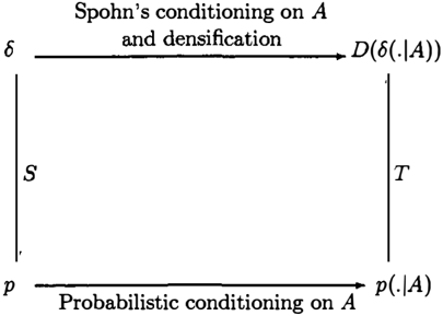
Suppose originally we have disbelief function 6, and after observing evidence (in the form of a proposition) A, and applying Spohn's rule of conditioning we get 6'. Further, suppose 6 was transformed to probability function p by S. Having observed A, we can condi­ tion p on the proposition and get p'. We will show that T(p') is almost the same as 6'. The result on con­ sistency of the transformation rules T and S can be summarized in the following scheme.

Theorem 3

Assume in this proof w, w' E A. We have: o(wJA) S: o(w'JA) iff o(w) :::;; o(w') iff S(o)(w) :::;; S(o)(w') i ff S(o)(wJA) :::;; S(o)(w'JA). The bi-directional inference chain is due by invoking, first, Spohn's conditioning definition, then the definition S and finally, the defini­ tion of probabilistic conditioning.

So if o(wJA) = o(w'JA) then S(o)(wJA) = S(o)(w'JA). And from the later equality, by definition ofT, we have T(S(o)(wJA)) = T(S(o)(w'JA)).

Now, to complete the proof we have to show that if o(wJA) < o(w'IA) then T(S(o)(wJA)) < T(S(o)(w'JA)).

Let o(w) = i, so o(w') > i. Recall notation G; ={wE UJ6(w) > i}. Let 8(6) = p, by lemma 2, we have p(w) > p(G;). We can rewrite

Note that for those wE G; nA, p(wJA) = �fA:l and for w ¢ G;nA, p(wJA) = 0. Sofromp(w) > p(G;), we have :!:4\ > p(�(A)) or using notation of conditional proba­ bility p(wJA) > p(G;nAJA). This is the condition to in­ crease rank parameter in definition ofT. So, applying transformation T for probability function p(.JA), we shall have T(p(.JA)(w) < T(p(.JA)(x) for all x E G;nA. Because of assumptions o(w') > i and w' E A, we have w' E G; n A. Thus, T(p(.JA)(w) < T(p(.JA)(w'). ·

Similarly, we can prove a result similar to Theorem 3 for the alternative method of probability updating, namely, Lewis' imaging. Lewis [11] motivated his for­ mulation of probabilistic imaging from the fact that conditional probabilities are not the same as proba­ bilities of conditionals except for trivial languages. To define an image of a probability function p on a propo­ sition A, one needs, in addition, a closeness relation among possible worlds. After observing A, the mass (probability) that p assigns to a world w ¢A is moved to the world(s) closest to w that is( are) in A. A disbe­ lief function readily provides a closeness relation. We can define the "distance" between two worlds w1, w2 by Jo(w1) - 6(w2)J. That means, having observed A, the mass of a world excluded by that observation will distributed evenly to the remained worlds of its class. Then Theorem 3 stills holds if (.JA) is understood as imaging on A instead of conditioning on A. Proof of that fact is similar to the proof of Theorem 3.

5 Summary and Conclusion

In this paper we describe two transformations from probability to Spohnian disbelief function and vice­ versa. In a departure from the widely used idea of re- lating disbelief values to infinitesimal probabilities i.e., E-rule, we adopt the principle of ordinal congruence as the basis for the transformations. Transformation T from probability to Spohnian disbelief is obtained if we couple the principle of congruence with the principle of minimal information loss. Transformation S from disbelief to probability function satisfies, in addition to the principle of congruence, the cautious attitude by allocating to less believed possible worlds the max­ imal probability that is permitted by the principle of congruence. We show that this pair of transformations are consistent with respect to conditionalization.

In the experimental works using E-rule as probability­ Spohnian disbelief transformations, a tension is how small should E be. On one hand, the results from [19, 20, 7] say that with an infinitesimal E, reasonings with probability and Spohnian disbelief are congruent. On the other hand, with E approaching 0, the transfor­ mation defined by E-rule becomes the trivial, i.e., any strictly positive probability is assigned disbelief degree zero. The experiments in [2, 8] are set up, partly, to examine the effect of E values on reasoning outcome. Unfortunately, the results of those experiments can not provide an unambiguous answer to that tension. In this paper, considering a transformation class broader than that defined by E-rule, we show that T is the best answer.

The transformation from non-probabilistic calculi to probability helps to connect the theories that lack de­ cision methods with the rich body of Bayesian decision theory developed for probability.

Another benefit of such a linkage is that it provides se­ mantics for the values of disbelief functions. For prob­ ability, we have the semantics of relative frequency and betting rates. A subjective interpretation of the stat& ment "probability of A is p" is the maximum price a risk neutral person would be willing pay to buy a lottery that pays $1.00 if A happens and nothing oth­ erwise. We do not know of any similar semantics for possibility values or Spohnian disbelief values. Indeed, Dubois and Prade [4, 5] take pains to explain that the information content of the numerical value of a possibility function is nothing but an ordinal ranking. Spohn [20] provides a link between his disbelief func­ tion and probability. But since this link is not formally stated, it cannot provide a useful semantic for values of disbelief functions via probabilistic semantics.

An advantage of Spohn's epistemic belief theory is computational simplicity. The human mind may not be designed for probabilistic computation. Common sense reasoning may not be probabilistic in nature. These assertions are supported by a large number of empirical studies in decision making [10]. Spohn's the-

ory was motivated partly from the notion of repre­ senting plain belief. On the other hand, a vast body of literature on the principle of maximization of ex­ pected utility suggested by von Neumann and Morgen­ stern [21] and Savage [12] tend to support the thesis that rational behavior is based on numerical probabil­ ities. So the transformations described in this paper offer a bridge between having plain beliefs and behav­ ing rationally. It also hints at the costs of rational behavior if one starts from plain beliefs.

References

1. E. Adams. The Logic of Conditionals, volume 86 of Synthese Library. D. Reidel, Dordrecht, 1975.
2. A. Darwiche and M. Goldszmidt. On the relation between kappa calculus and probabilistic reason­ ing. In R. Lopez de Mantaras and D. Poole, ed­ itors, Uncertainty in Artificial Intelligence. Mor­ gan Kaufmann, 1994.
3. M. Delgado and S. Moral. On the concept of possibility-probability consistency. Fuzzy Sets and Syste11Ui, 21:311-318, 1987.
4. D. Dubois and H. Prade. Epistemic entrench­ ment and possibilistic logic. Artificial Intelligence, 50:223-239, 1991.
5. D. Dubois and H. Prade. Fuzzy numbers: an overview. In D. Dubois, H. Prade, and R. Yager, editors, Readings in Fuzzy Sets for Intelligent Sys­ te11Ui, pages 112-148. Morgan Kaufmann, 1993.
6. [6) D. Dubois, H. Prade, and S. Sandri. On possibil­ ity/ probability transformations. In R. Lowen and M. Roubens, editors, Fuzzy Logic: State of the Art, pages 103-112. Kluwer Academic Publisher, 1993.
7. [7) M. Goldszmidt and J. Pearl. Reasoning with qualitative probabilities can be tractable. In D. Dubois, M. P. Wellman, B. D'Ambrosio, and P. Smets, editors, Uncertainty in Artificial In­ telligence: Proceedings of the Eighth Conference, pages 112-120. Morgan Kaufmann, 1992.
8. M. Henrion, G. Provan, B. Del Favero, and G. Sanders. An experimental comparison of nu­ merical and qualitative probabilistic reasoning. In R. Lopez de Mantaras and D. Poole, editors, Un­ certainty in Artificial Intelligence. Morgan Kauf­ mann, 1994.
9. [9) D. Hunter. Parallel belief revision. In R. Shachter, T. Levitt, L. Kana!, and J. Lemmer, editors, Un­ certainty in Artificial Intelligence, volume 4. El­ sevier Science, 1990.
10. D. Kahneman, P. Slovic, and A. Tversky. Judg­ ment Under Uncertainty: Heuristics and Biases. Cambridge University Press, New York, 1982.
11. D. Lewis. Probabilities of conditionals and condi­ tional probabilities. Philosophical Review, 85:297315, 1976. Reprinted in D. Lewis, Philosophical Papers, Oxford University Press, 1986.
12. [12) L. J. Savage. The Foundations of Statistics. Dover, New York, second edition, 1972.
13. P. P. Shenoy. On spohn's revision of belief. In­ ternational Journal of Approximate Reasoning, 5:149-181, 1991.
14. [14) P. P. Shenoy. Using possibility theory in ex­ pert system. Fuzzy Sets and Syste11Ui, 52:129-142, 1992.
15. P. P. Shenoy. Valuation-based systems: A frame­ work for managing uncertainty in expert systems. In L. A. Zadeh and J. Kacprzyk, editors, Fuzzy Logic for Management of Uncertainty, pages 83104. John Wiley & Son, 1992.
16. P. P. Shenoy. Uncertain reasoning. Unpublished BUS934 Lecture Note, School of Business, Uni­ versity of Kansas, Fall, 1998.
17. P. P. Shenoy and G. Shafer. An axiomatic frame­ work for bayesian and belief function propaga­ tion. In R. Shachter, T. Levitt, L. Kana!, and J. Lemmer, editors, Uncertainty in Artificial In­ telligence, volume 4. Elsevier Science, 1990.
18. [18) P. Snow. The emergence of ordered belief from ini­ tial ignorance. In Proceedings of Twelfth National Conference on Artificial Intelligence, AAAI-94, volume 1, pages 281-286. AAAI Press/ MIT Press, 1994.
19. [19) W. Spohn. Ordinal conditional function: A dy­ namic theory of epistemic states. In L. Harper and B. Skyrms, editors, Causation in Decision, Be­ lief Change and Statistics, pages 105-134. Kluwer Academic Publisher, 1988.
20. W. Spohn. A general non-probabilistic theory of inductive reasoning. In R. Shachter, T. Levitt, L. Kana!, and J. Lemmer, editors, Uncertainty in Artificial Intelligence, volume 4. Elsevier Science, 1990.
21. J. von Neumann and 0. Morgenstern. Theory of Games and Economic Behavior. Princeton Uni­ versity Press, Princeton, NJ, 3 edition, 1953.