Range and Roots

Two Common Patterns for Specifying and Propagating

Counting and Occurrence Constraints

Christian Bessiere LIRMM, CNRS and U. Montpellier Montpellier, France [email protected]

Brahim Hnich

Izmir University of Economics Izmir, Turkey [email protected]

: ∗

Emmanuel Hebrard 4C and UCC Cork, Ireland [email protected]

Zeynep Kiziltan

Department of Computer Science Univ. di Bologna, Italy [email protected]

Toby Walsh NICTA and UNSW Sydney, Australia [email protected]

Keywords: Constraint programming, constraint satisfaction, global constraints, open global constraints, decompositions

Abstract

We propose Range and Roots which are two common patterns useful for specifying a wide range of counting and occurrence constraints. We design specialised propagation algorithms for these two patterns. Counting and occurrence constraints specified using these patterns thus directly inherit a propagation algorithm. To illustrate the capabilities of the Range and Roots constraints, we specify a number of global constraints taken from the literature. Preliminary experiments demonstrate that propagating counting and occurrence constraints using these two patterns leads to a small loss in performance when compared to specialised global constraints and is competitive with alternative decompositions using elementary constraints.

∗ This paper is a compilation and an extension of [10], [11], and [12]. The first author was supported by the ANR project ANR-06-BLAN-0383-02.

1 Introduction

Global constraints are central to the success of constraint programming [28]. Global constraints allow users to specify patterns that occur in many problems, and to exploit efficient and effective propagation algorithms for pruning the search space. Two common types of global constraints are counting and occurrence constraints. Occurrence constraints place restrictions on the occurrences of particular values. For instance, we may wish to ensure that no value used by one set of variables occurs in a second set. Counting constraints, on the other hand, restrict the number of values or variables meeting some condition. For example, we may want to limit the number of distinct values assigned to a set of variables. Many different counting and occurrences constraints have been proposed to help model a wide range of problems, especially those involving resources (see, for example, [25, 4, 26, 3, 5]).

In this paper, we will show that many such constraints can be specified by means of two new global constraints, Range and Roots together with some standard elementary constraints like subset and set cardinality. These two new global constraints capture the familiar notions of image and domain of a function. Understanding such notions does not require a strong background in constraint programming. A basic mathematical background is sufficient to understand these constraints and use them to specify other global constraints. We will show, for example, that Range and Roots are versatile enough to allow specification of open global constraints, a recent kind of global constraints for which the set of variables involved is not known in advance.

Specifications made with Range and Roots constraints are executable. We show that efficient propagators can be designed for the Range and Roots constraints. We give an efficient algorithm for propagating the Range constraint based on a flow algorithm. We also prove that it is intractable to propagate the Roots constraint completely. We therefore propose a decomposition of the Roots constraint that can propagate it partially in linear time. This decomposition does not destroy the global nature of the Roots constraint as in many situations met in practice, it prunes all possible values. The proposed propagators can easily be incorporated into a constraint toolkit.

We show that specifying a global constraint using Range and Roots provides us with an reasonable method to propagate counting and occurrence constraints. There are three possible situations. In the first, the global nature of the Range and Roots constraints is enough to capture the global nature of the given counting or occurrence constraint, and propagation is not hindered. In the second situation, completely propagating the counting or occurrence constraint is NP-hard. We must accept some loss of propagation if propagation is to be tractable. Using Range and Roots is then one means to propagate the counting or occurrence constraint partially. In the third situation, the global constraint can be propagated completely in polynomial time but using Roots and Range hinders propagation. In this case, if we want to achieve full propagation, we need to develop a specialised propagation algorithm.

We also show that decomposing occurrence constraints and counting constraints using the Range and Roots constraints performs well in practice. Our experiments on random CSPs and a on real world problem from CSPLib demonstrate that propagating counting and occurrence constraints using the Range and Roots constraints leads to a small loss in performance when compared to specialised global constraints and is competitive with

alternative decompositions into more elementary constraints.

The rest of the paper is organised as follows. Section 2 gives the formal background. Section 3 defines the Range and Roots constraints and gives a couple of examples to illustrate how global constraints can be decomposed using these two constraints. In Section 4, we propose a polynomial algorithm for the Range constraint. In Section 5, we give a complete theoretical analysis of the Roots constraint and our decomposition of it, and we discuss implementation details. Section 6 gives many examples of counting and occurrence constraints that can be specified using the Range and Roots constraints. Experimental results are presented in Section 7. Finally, we end with conclusions in Section 8.

2 Formal background

A constraint satisfaction problem consists of a set of variables, each with a finite domain of values, and a set of constraints specifying allowed combinations of values for subsets of variables. We use capitals for variables (e.g. X , Y and S ), and lower case for values (e.g. v and w ). We write D ( X ) for the domain of a variable X . A solution is an assignment of values to the variables satisfying the constraints. A variable is ground when it is assigned a value. We consider both integer and set variables. A set variable S is often represented by its lower bound lb ( S ) which contains the definite elements (that must belong to the set) and an upper bound ub ( S ) which also contains the potential elements (that may or may not belong to the set).

Constraint solvers typically explore partial assignments enforcing a local consistency property using either specialised or general purpose propagation algorithms. Given a constraint C , a bound support on C is a tuple that assigns to each integer variable a value between its minimum and maximum, and to each set variable a set between its lower and upper bounds which satisfies C . A bound support in which each integer variable is assigned a value in its domain is called a hybrid support . If C involves only integer variables, a hybrid support is a support . A value (resp. set of values) for an integer variable (resp. set variable) is bound or hybrid consistent with C iff there exists a bound or hybrid support assigning this value (resp. set of values) to this variable. A constraint C is bound consistent ( BC ) iff for each integer variable X i , its minimum and maximum values belong to a bound support, and for each set variable S j , the values in ub ( S j ) belong to S j in at least one bound support and the values in lb ( S j ) are those from ub ( S j ) that belong to S j in all bound supports. A constraint C is hybrid consistent ( HC ) iff for each integer variable X i , every value in D ( X i ) belongs to a hybrid support, and for each set variable S j , the values in ub ( S j ) belong to S j in at least one hybrid support, and the values in lb ( S j ) are those from ub ( S j ) that belong to S j in all hybrid supports. A constraint C involving only integer variables is generalised arc consistent ( GAC ) iff for each variable X i , every value in D ( X i ) belongs to a support. If all variables in C are integer variables, hybrid consistency reduces to generalised arc consistency, and if all variables in C are set variables, hybrid consistency reduces to bound consistency.

To illustrate these different concepts, consider the constraint C ( X 1 , X 2 , T ) that holds iff the set variable T is assigned exactly the values used by the integer variables X 1 and X 2 . Let D ( X 1 ) = { 1 , 3 } , D ( X 2 ) = { 2 , 4 } , lb ( T ) = { 2 } and ub ( T ) = { 1 , 2 , 3 , 4 } . BC

does not remove any value since all domains are already bound consistent (value 2 was considered as possible for X 1 because BC deals with bounds). On the other hand, HC removes 4 from D ( X 2 ) and from ub ( T ) as there does not exist any tuple satisfying C in which X 2 does not take value 2.

We will compare local consistency properties applied to (sets of) logically equivalent constraints, c 1 and c 2 . As in [17], a local consistency property Φ on c 1 is as strong as Ψ on c 2 iff, given any domains, if Φ holds on c 1 then Ψ holds on c 2 ; Φ on c 1 is stronger than Ψ on c 2 iff Φ on c 1 is as strong as Ψ on c 2 but not vice versa; Φ on c 1 is equivalent to Ψ on c 2 iff Φ on c 1 is as strong as Ψ on c 2 and vice versa; Φ on c 1 is incomparable to Ψ on c 2 iff Φ on c 1 is not as strong as Ψ on c 2 and vice versa.

A total function F from a source set S into a target set T is denoted by F : S -→ T . The set of all elements in S that have the same image j ∈ T is F -1 ( j ) = { i : F ( i ) = j } . The image of a set S ⊆ S under F is F ( S ) = ⋃ i ∈ S F ( i ), whilst the domain of a set T ⊆ T under F is F -1 ( T ) = ⋃ j ∈ T F -1 ( j ). Throughout, we will view a set of integer variables, X 1 to X n as a function X : { 1 , .., n } -→ ⋃ i = n i =1 D ( X i ). That is, X ( i ) is the value of X i .

3 Two useful patterns: Range and Roots

Many counting and occurrence constraints can be specified using simple non-global constraints over integer variables (like X ≤ m ), simple non-global constraints over set variables (like S 1 ⊆ S 2 or | S | = k ) available in most constraint solvers, and two special global constraints acting on sequences of variables: Range and Roots . Range captures the notion of image of a function and Roots captures the notion of domain . Specification with Range and Roots is executable. It permits us to decompose other global constraints into more primitive constraints.

Given a function X representing a set of integer variables, X 1 to X n , the Range constraint holds iff a set variable T is the image of another set variable S under X .

The Roots constraint holds iff a set variable S is the domain of the another set variable T under X .

Range and Roots are not exact inverses. A Range constraint can hold, but the corresponding Roots constraint may not, and vice versa. For instance, Range ([1 , 1] , { 1 } , { 1 } ) holds but not Roots ([1 , 1] , { 1 } , { 1 } ) since X -1 (1) = { 1 , 2 } , and Roots ([1 , 1 , 1] , { 1 , 2 , 3 } , { 1 , 2 } ) holds but not Range ([1 , 1 , 1] , { 1 , 2 , 3 } , { 1 , 2 } ) as no X i is assigned to 2.

Before showing how to propagate Range and Roots efficiently, we give two examples that illustrate how some counting and occurrence global constraints from [2] can be specified using Range and Roots .

The NValue constraint counts the number of distinct values used by a sequence of variables [22, 8, 7]. NValue ([ X 1 , .., X n ] , N ) holds iff N = |{ X i | 1 ≤ i ≤ n }| . A way to implement this constraint is with a Range constraint:

The AtMost constraint is one of the oldest global constraints [32]. The AtMost constraint puts an upper bound on the number of variables using a particular value. AtMost ([ X 1 , .., X n ] , d, N ) holds iff |{ i | X i = d }| ≤ N . It can be decomposed using a Roots constraint.

These two examples show that it can be quite simple to decompose global constraints using Range and Roots . As we will show later, some other global constraints will require the use of both Range and Roots in the same decomposition. The next sections show how Range and Roots can be propagated efficiently.

4 Propagating the Range constraint

Enforcing hybrid consistency on the Range constraint is polynomial. This can be done using a maximum network flow problem. In fact, the Range constraint can be decomposed using a global cardinality constraint ( Gcc ) for which propagators based on flow problems already exist [26, 24]. But the Range constraint does not need the whole power of maximum network flow problems, and thus HC can be enforced on it at a lower cost than that of calling a Gcc propagator. In this section, we propose an efficient way to enforce HC on Range . To simplify the presentation, the use of the flow is limited to a constraint that performs only part of the work needed for enforcing HC on Range . This constraint, that we name Occurs ([ X 1 , . . . , X n ] , T ), ensures that all the values in the set variable T are used by the integer variables X 1 to X n :

We first present an algorithm for achieving HC on Occurs (Section 4.1), and then use this to propagate the Range constraint (Section 4.2).

4.1 Hybrid consistency on Occurs

We achieve HC on Occurs ([ X 1 , . . . , X n ] , T ) using a network flow.

4.1.1 Building the network flow

We use a unit capacity network [1] in which capacities between two nodes can only be 0 or 1. This is represented by a directed graph where an arc from node x to node y means that a maximum flow of 1 is allowed between x and y while the absence of an arc means that

z

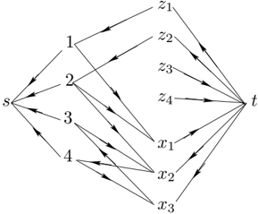
the maximum flow allowed is 0. The unit capacity network G C = ( N,E ) of the constraint C = Occurs ([ X 1 , . . . , X n ] , T ) is built in the following way. N = { s } ∪ N 1 ∪ N 2 ∪ { t } , where s is a source node, t is a sink node, N 1 = { v | v ∈ ⋃ D ( X i ) } and N 2 = { z v | v ∈ ⋃ D ( X i ) } ∪ { x i | i ∈ [1 ..n ] } . The set of arcs E is as follows:

G C is quadripartite, i.e., E ⊆ ( { s } × N 1 ) ∪ ( N 1 × N 2 ) ∪ ( N 2 ×{ t } ). In Fig. 1, we depict the network G C of the constraint C = Occurs ([ X 1 , X 2 , X 3 ] , T ) with D ( X 1 ) = { 1 , 2 } , D ( X 2 ) = { 2 , 3 , 4 } , D ( X 3 ) = { 3 , 4 } , lb ( T ) = { 3 , 4 } and ub ( T ) = { 1 , 2 , 3 , 4 } . The intuition behind this graph is that when a flow uses an arc from a node v to a node x i this means that X i is assigned v , and when a flow uses the arc ( v, z v ) this means that v is not necessarily used by the X i 's. 1 In Fig. 1 nodes 3 and 4 are linked only to nodes x 2 and x 3 , that is, values 3 and 4 must necessarily be taken by one of the variables X i (3 and 4 belong to lb ( T )). On the contrary, nodes 1 and 2 are also linked to nodes z 1 and z 2 because values 1 and 2 do not have to be taken by a X i (they are not in lb ( T )).

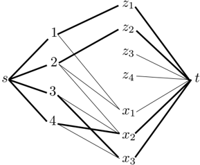
In the particular case of unit capacity networks, a flow is any set E ′ ⊆ E : any arc in E ′ is assigned 1 and the arcs in E \ E ′ are assigned 0. A feasible flow from s to t in G C is a subset E f of E such that ∀ n ∈ N \{ s, t } the number of arcs of E f entering n is equal to the number of arcs of E f going out of n , that is, |{ ( n ′ , n ) ∈ E f }| = |{ ( n, n ′′ ) ∈ E f }| . The value of the flow E f from s to t , denoted val ( E f , s, t ), is val ( E f , s, t ) = |{ n | ( s, n ) ∈ E f }| . A maximum flow from s to t in G C is a feasible flow E M such that there does not exist a feasible flow E f , with val ( E f , s, t ) > val ( E M , s, t ). A maximum flow for the network of Fig. 1 is given in Fig. 2. By construction a feasible flow cannot have a value greater than | N 1 | and cannot contain two arcs entering a node x i from N 2 . Hence, we can define a function ϕ linking feasible flows and partial instantiations on the X i 's. Given any feasible flow E f from s to t in G C , ϕ ( E f ) = { ( X i , v ) | ( v, x i ) ∈ E f } . The maximum flow

1 Note that in our presentation of the graph, the edges go from the nodes representing the values to the nodes representing the variables. This is the opposite to the direction used in the presentation of network flows for propagators of the AllDifferent or Gcc constraints [25, 26].

z

in Fig. 2 corresponds to the instantiation X 2 = 4 , X 3 = 3. The way G C is built induces the following theorem.

Theorem 1 Let G C = ( N,E ) be the capacity network of a constraint C = Occurs ([ X 1 , . . . , X n ] , T ) .

1. A value v in the domain D ( X i ) for some i ∈ [1 ..n ] is HC iff there exists a flow E f from s to t in G C with val ( E f , s, t ) = | N 1 | and ( v, x i ) ∈ E f
2. If the X i 's are HC, T is HC iff ub ( T ) ⊆ ⋃ i D ( X i )

/negationslash

/negationslash

(1. ⇐ ) Let E M be a flow from s to t in G C with ( v, x i ) ∈ E M and val ( E M , s, t ) = | N 1 | . By construction of G C , we are guaranteed that all nodes in N 1 belong to an arc in E M ∩ ( N 1 × N 2 ), and that for every value w ∈ lb ( T ), { y | ( w, y ) ∈ E } ⊆ { x i | i ∈ [1 ..n ] } . Thus, for each w ∈ lb ( T ) , ∃ X j | ( X j , w ) ∈ ϕ ( E M ). Hence, any extension of ϕ ( E M ) where each unassigned X j takes any value in D ( X j ) and T = lb ( T ) is a solution of C with X i = v .

Proof. (1. ⇒ ) Let I be a solution for C with ( X i , v ) ∈ I . Build the following flow H : Put ( v, x i ) in H ; ∀ w ∈ I [ T ] , w = v , take a variable X j such that ( X j , w ) ∈ I (we know there is at least one since I is solution), and put ( w, x j ) in H ; ∀ w ′ / ∈ I [ T ] , w ′ = v , add ( w ′ , z w ′ ) to H . Add to H the edges from s to N 1 and from N 2 to t so that we obtain a feasible flow. By construction, all w ∈ N 1 belong to an edge of H . So, val ( H,s,t ) = | N 1 | and H is a maximum flow with ( v, x i ) ∈ H .

(2. ⇒ ) If T is HC, all values in ub ( T ) appear in at least one solution tuple. Since C

(2. ⇐ ) Let ub ( T ) ⊆ ⋃ i D ( X i ). Since all X i 's are HC, we know that each value v in ⋃ i D ( X i ) is taken by some X i in at least one solution tuple I . Build the tuple I ′ so that I ′ [ X i ] = I [ X i ] for each i ∈ [1 ..n ] and I ′ [ T ] = I [ T ] ∪ { v } . I ′ is still solution of C . So, ub ( T ) is as tight as it can be wrt HC. In addition, since all X i 's are HC, this means that in every solution tuple I , for each v ∈ lb ( T ) there exists i such that I [ X i ] = v . So, lb ( T ) is HC. ✷

ensures that T ⊆ ⋃ i { X i } , ub ( T ) cannot contain a value appearing in none of the D ( X i ).

Following Theorem 1, we need a way to check which edges belong to a maximum flow. Residual graphs are useful for this task. Given a unit capacity network G C and

z

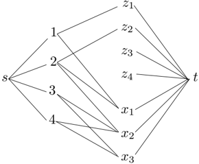
a maximal flow E M from s to t in G C , the residual graph R G C ( E M ) = ( N,E R ) is the directed graph obtained from G C by reversing all arcs belonging to the maximum flow E M ; that is, E R = { ( x, y ) ∈ E \ E M } ∪ { ( y, x ) | ( x, y ) ∈ E ∩ E M } . Given the network G C of Fig. 1 and the maximum flow E M of Fig. 2, R G C ( E M ) is depicted in Fig. 3. Given a maximum flow E M from s to t in G C , given ( x, y ) ∈ N 1 × N 2 ∩ E \ E M , there exists a maximum flow containing ( x, y ) iff ( x, y ) belongs to a cycle in R G C ( E M ) [29]. Furthermore, finding all the arcs ( x, y ) that do not belong to a cycle in a graph can be performed by building the strongly connected components of the graph. We see in Fig. 3 that the arcs (1 , x 1 ) and (2 , x 1 ) belong to a cycle. So, they belong to some maximum flow and ( X 1 , 1) and ( X 1 , 2) are hybrid consistent. (2 , x 2 ) does not belong to any cycle. So, ( X 2 , 2) is not HC.

4.1.2 Using the network flow for achieving HC on Occurs

We now have all the tools for achieving HC on any Occurs constraint. We first build G C . We compute a maximum flow E M from s to t in G C ; if val ( E M , s, t ) < | N 1 | , we fail. Otherwise we compute R G C ( E M ), build the strongly connected components in R G C ( E M ), and remove from D ( X i ) any value v such that ( v, x i ) belongs to neither E M nor to a strongly connected component in R G C ( E M ). Finally, we set ub ( T ) to ub ( T ) ∩ ⋃ i D ( X i ). Following Theorem 1 and properties of residual graphs, this algorithm enforces HC on Occurs ([ X 1 , .., X n ] , T ).

Complexity. Building G C is in O ( nd ) where d is the maximum domain size. We need then to find a maximum flow E M in G C . This can be done in two sub-steps. First, we use the arc ( v, z v ) for each v / ∈ lb ( T ) (in O ( | ⋃ i D ( X i ) | )). Afterwards, we compute a maximum flow on the subgraph composed of all paths traversing nodes w with w ∈ lb ( T ) (because there is no arc ( w, z w ) in G C for such w ). The complexity of finding a maximum flow in a unit capacity network is in O ( √ k · e ) if k is the number of nodes and e the number of edges. This gives a complexity in O ( √ | lb ( T ) | · | lb ( T ) | · n ) for this second sub-step. Building the residual graph and computing the strongly connected components is in O ( nd ). Extracting the HC domains for the X i 's is direct. There remains to compute BC on T , which takes O ( nd ). Therefore, the total complexity is in O ( nd + n · | lb ( T ) | 3 / 2 ).

Algorithm 1 : Hybrid consistency on Range

procedure Propag-Range ([ X 1 , . . . , X n ] , S, T );

• Introduce the set of integer variables Y = { Y i | i ∈ ub ( S ) } , 1 with D ( Y i ) = D ( X i ) ∪ { dummy } ;
• Achieve hybrid consistency on the constraint Occurs ( Y, T ); 2
• Achieve hybrid consistency on the constraints i ∈ S ↔ Y i ∈ T , for all Y i ∈ Y ; 3
• Achieve GAC on the constraints ( Y i = dummy ) ∨ ( Y i = X i ), for all Y i ∈ Y ; 4

Incrementality. In constraint solvers, constraints are usually maintained in a locally consistent state after each modification (restriction) of the domains of the variables. It is thus interesting to consider the total complexity of maintaining HC on Occurs after an arbitrary number of restrictions on the domains (values removed from D ( X i ) and ub ( T ), or added to lb ( T )) as we descend a branch of a backtracking search tree. Whereas some constraints are completely incremental (i.e., the total complexity after any number of restrictions is the same as the complexity of one propagation), this is not the case for constraints based on flow techniques like AllDifferent or Gcc [25, 26]. They potentially require the computation of a new maximum flow after each modification. Restoring a maximum flow from one that lost p edges is in O ( p · e ). If values are removed one by one ( nd possible times), and if each removal affects the current maximum flow, the overall complexity over a sequence of restrictions on X i 's, S , T , is in O ( n 2 d 2 ).

4.2 Hybrid consistency on Range

Enforcing HC on Range ([ X 1 , . . . , X n ] , S, T ) can be done by decomposing it as an Occurs constraint on new variables Y i and some channelling constraints ([16]) linking T and the Y i 's to S and the X i 's. Interestingly, we do not need to maintain HC on the decomposition but just need to propagate the constraints in one pass .

The algorithm Propag-Range , enforcing HC on the Range constraint, is presented in Algorithm 1. In line 1, a special encoding is built, where a Y i is introduced for each X i with index in ub ( S ). The domain of a Y i is the same as that of X i plus a dummy value. The dummy value works as a flag. If Occurs prunes it from D ( Y i ) this means that Y i is necessary in Occurs to cover lb ( T ). Then, X i is also necessary to cover lb ( T ) in Range . In line 1, HC on Occurs removes a value from a Y i each time it contains other values that are necessary to cover lb ( T ) in every solution tuple. HC also removes values from ub ( T ) that cannot be covered by any Y i in a solution. Line 1 updates the bounds of S and the domain of Y i 's. Finally, in line 1, the channelling constraints between Y i and X i propagate removals on X i for each i which belongs to S in all solutions.

Theorem 2 The algorithm Propag-Range is a correct algorithm for enforcing HC on Range , that runs in O ( nd + n · | lb ( T ) | 3 / 2 ) time, where d is the maximal size of X i domains.

Proof. Soundness . A value v is removed from D ( X i ) in line 1 if it is removed from Y i together with dummy in lines 1 or 1. If a value v is removed from Y i in line 1, this means that any tuple on variables in Y covering lb ( T ) requires that Y i takes a value from D ( Y i )

other than v . So, we cannot find a solution of Range in which X i = v since lb ( T ) must be covered as well. A value v is removed from D ( Y i ) in line 1 if i ∈ lb ( S ) and v /negationslash∈ ub ( T ). In this case, Range cannot be satisfied by a tuple where X i = v . If a value v is removed from ub ( T ) in line 1, none of the tuples of values for variables in Y covering lb ( T ) can cover v as well. Since variables in Y duplicate variables X i with index in ub ( S ), there is no hope to satisfy Range if v is in T . Note that ub ( T ) cannot be modified in line 1 since Y contains only variables Y i for which i was in ub ( S ). If a value v is added to lb ( T ) in line 1, this is because there exists i in lb ( S ) such that D ( Y i ) ∩ ub ( T ) = { v } . Hence, v is necessarily in T in all solutions of Range . An index i can be removed from ub ( S ) only in line 1. This happens when the domain of Y i does not intersect ub ( T ). In such a case, this is evident that a tuple where i ∈ S could not satisfy Range since X i could not take a value in T . Finally, if an index i is added to lb ( S ) in line 1, this is because D ( Y i ) is included in lb ( T ), which means that the dummy value has been removed from D ( Y i ) in line 1. This means that Y i takes a value from lb ( T ) in all solutions of Occurs . X i also has to take a value from lb ( T ) in all solutions of Range .

Completeness Suppose that a value v is not pruned from D ( X i ) after line 1 of PropagRange . If Y i ∈ Y , we know that after line 1 there was an instantiation I on Y and T , solution of Occurs with I [ Y i ] = v or with Y i = dummy (thanks to the channelling constraints in line 1). We can build the tuple I ′ on X 1 , ..X n , S, T where X i takes value v , every X j with j ∈ ub ( S ) and I [ Y j ] ∈ I [ T ] takes I [ Y j ], and the remaining X j 's take any value in their domain. T is set to I [ T ] plus the values taken by X j 's with j ∈ lb ( S ). These values are in ub ( T ) thanks to line 1. Finally, S is set to lb ( S ) plus the indices of the Y j 's with I [ Y j ] ∈ I [ T ]. These indices are in ub ( S ) since the only j 's removed from ub ( S ) in line 1 are such that D ( Y j ) ∩ ub ( T ) = ∅ , which prevents I [ Y j ] from taking a value in I [ T ]. Thus I ′ is a solution of Range with I ′ [ X i ] = v . We have proved that the X i 's are hybrid consistent after Propag-Range .

Suppose a value i ∈ ub ( S ) after line 1. Thanks to constraint in line 1 we know there exists v in D ( Y i ) ∩ ub ( T ), and so, v ∈ D ( X i ) ∩ ub ( T ). Now, X i is hybrid consistent after line 1. Thus X i = v belongs to a solution of Range . If we modify this solution by putting i in S and v in T (if not already there), we keep a solution.

Completeness on lb ( S ), lb ( T ) and ub ( T ) is proved in a similar way.

Complexity . The important thing to notice in Propag-Range is that constraints in lines 1-1 are propagated in sequence. Thus, Occurs is propagated only once, for a complexity in O ( nd + n · | lb ( T ) | 3 / 2 ). Lines 1, 1, and 1 are in O ( nd ). Thus, the complexity of PropagRange is in O ( nd + n · | lb ( T ) | 3 / 2 ). This reduces to linear time complexity when lb ( T ) is empty.

Incrementality . The overall complexity over a sequence of restrictions on X i 's, S and T is in O ( n 2 d 2 ). (See incrementality of Occurs in Section 4.1.) ✷

Note that the Range constraint can be decomposed using the Gcc constraint. However, propagation on such a decomposition is in O ( n 2 d + n 2 . 66 ) time complexity (see [24]). Propag-Range is thus significantly cheaper.

5 Propagating the Roots constraint

We now give a thorough theoretical analysis of the Roots constraint. In Section 5.1, we provide a proof that enforcing HC on Roots is NP-hard in general. Section 5.2 presents a decomposition of the Roots constraint that permits us to propagate the Roots constraint partially in linear time. Section 5.3 shows that in many cases this decomposition does not destroy the global nature of the Roots constraint as enforcing HC on the decomposition achieves HC on the Roots constraint. Section 5.4 shows that we can obtain BC on the Roots constraint by enforcing BC on its decomposition. Finally, we provide some implementation details in Section 5.5.

5.1 Complete propagation

Unfortunately, propagating the Roots constraint completely is intractable in general. Whilst we made this claim in [10], a proof has not yet been published. For this reason, we give one here.

Theorem 3 Enforcing HC on the Roots constraint is NP-hard.

Proof. We transform 3Sat into the problem of the existence of a solution for Roots . Finding a hybrid support is thus NP-hard. Hence enforcing HC on Roots is NP-hard. Let ϕ = { c 1 , . . . , c m } be a 3CNF on the Boolean variables x 1 , . . . , x n . We build the constraint Roots ([ X 1 , . . . , X n + m ] , S, T ) as follows. Each Boolean variable x i is represented by the variable X i with domain D ( X i ) = { i, -i } . Each clause c p = x i ∨ ¬ x j ∨ x k is represented by the variable X n + p with domain D ( X n + p ) = { i, -j, k } . We build S and T in such a way that it is impossible for both the index i of a Boolean variable x i and its complement -i to belong to T . We set lb ( T ) = ∅ and ub ( T ) = ⋃ n i =1 { i, -i } , and lb ( S ) = ub ( S ) = { n + 1 , . . . , n + m } . An interpretation M on the Boolean variables x 1 , . . . , x n is a model of ϕ iff the tuple τ in which τ [ X i ] = i iff M [ x i ] = 0 can be extended to a solution of Roots . (This extension puts in T value i iff M [ x i ] = 1 and assigns X n + p with the value corresponding to the literal satisfying c p in M .) ✷

We thus have to look for a lesser level of consistency for Roots or for particular cases on which HC is polynomial. We will show that bound consistency is tractable and that, under conditions often met in practice (e.g. one of the last two arguments of Roots is ground), enforcing HC is also.

5.2 A decomposition of Roots

To show that Roots can be propagated tractably, we will give a straightforward decomposition into ternary constraints that can be propagated in linear time. This decomposition does not destroy the global nature of the Roots constraint since enforcing HC on the decomposition will, in many cases, achieve HC on the original Roots constraint, and since in all cases, enforcing BC on the decomposition achieves BC on the original Roots constraint. Given Roots ([ X 1 , .., X n ] , S, T ), we decompose it into the implications:

where i ∈ [1 ..n ]. We have to be careful how we implement such a decomposition in a constraint solver. First, some solvers will not achieve HC on such constraints (see Sec 5.5 for more details). Second, we need an efficient algorithm to be able to propagate the decomposition in linear time. As we explain in more detail in Sec 5.5, a constraint solver could easily take quadratic time if it is not incremental.

We first show that this decomposition prevents us from propagating the Roots constraint completely. However, this is to be expected as propagating Roots completely is NP-hard and this decomposition is linear to propagate. In addition, as we later show, in many circumstances met in practice, the decomposition does not in fact hinder propagation.

Theorem 4 HC on Roots ([ X 1 , .., X n ] , S, T ) is strictly stronger than HC on i ∈ S → X i ∈ T , and X i ∈ T → i ∈ S for all i ∈ [1 ..n ] .

Proof. Consider X 1 ∈ { 1 , 2 } , X 2 ∈ { 3 , 4 } , X 3 ∈ { 1 , 3 } , X 4 ∈ { 2 , 3 } , lb ( S ) = ub ( S ) = { 3 , 4 } , lb ( T ) = ∅ , and ub ( T ) = { 1 , 2 , 3 , 4 } . The decomposition is HC. However, enforcing HC on Roots will prune 3 from D ( X 2 ). ✷

In fact, enforcing HC on the decomposition achieves a level of consistency between BC and HC on the original Roots constraint. Consider X 1 ∈ { 1 , 2 , 3 } , X 2 ∈ { 1 , 2 , 3 } , lb ( S ) = ub ( S ) = { 1 , 2 } , lb ( T ) = {} , and ub ( T ) = { 1 , 3 } . The Roots constraint is BC. However, enforcing HC on the decomposition will remove 2 from the domains of X 1 and X 2 . In the next section, we identify exactly when the decomposition achieves HC on Roots .

5.3 Some special cases

Many of the counting and occurrence constraints do not use the Roots constraint in its more general form, but have some restrictions on the variables S , T or X i 's. For example, it is often the case that T or S are ground. We select four important cases that cover many of these uses of Roots and show that enforcing HC on Roots is then tractable.

• C1. ∀ i ∈ lb ( S ) , D ( X i ) ⊆ lb ( T )
• C2. ∀ i / ∈ ub ( S ) , D ( X i ) ∩ ub ( T ) = ∅
• C3. X 1 , .., X n are ground

C4. T is ground

We will show that in any of these cases, we can achieve HC on Roots simply by propagating the decomposition.

Theorem 5 If one of the conditions C 1 to C 4 holds, then enforcing HC on i ∈ S → X i ∈ T , and X i ∈ T → i ∈ S for all i ∈ [1 ..n ] achieves HC on Roots ([ X 1 , .., X n ] , S, T ) .

Proof. Our proof will exploit the following properties that are guaranteed to hold when we have enforced HC on the decomposition.

• P1 if D ( X i ) ⊆ lb ( T ) then i ∈ lb ( S )
• P2 if D ( X i ) ∩ ub ( T ) = ∅ then i / ∈ ub ( S )
• P3 if i ∈ lb ( S ) then D ( X i ) ⊆ ub ( T )
• P4 if i / ∈ ub ( S ) then D ( X i ) ∩ lb ( T ) = ∅
• P5 if D ( X i ) = { v } and i ∈ lb ( S ) then v ∈ lb ( T )
• P6 if D ( X i ) = { v } and i / ∈ ub ( S ) then v / ∈ ub ( T )
• P7 if i is added to lb ( S ) by the constraint X i ∈ T → i ∈ S then D ( X i ) ⊆ lb ( T )
• P8 if i is deleted from ub ( S ) by the constraint i ∈ S → X i ∈ T then D ( X i ) ∩ ub ( T ) = ∅

Soundness. Immediate.

Completeness. We assume that one of the conditions C1-C4 holds and the decomposition is HC. We will first prove that the Roots constraint is satisfiable. Then, we will prove that, for any X i , all the values in D ( X i ) belong to a solution of Roots , and that the bounds on S and T are as tight as possible.

We prove that the Roots constraint is satisfiable. Suppose that one of the conditions C1-C4 holds and that the decomposition is HC. Build the following tuple τ of values for the X i , S , and T . Initialise τ [ S ] and τ [ T ] with lb ( S ) and lb ( T ) respectively. Now, let us consider the four conditions separately.

(C1) For each i ∈ τ [ S ], choose any value v in D ( X i ) for τ [ X i ]. From the assumption and from property P7 we deduce that v is in lb ( T ), and so in τ [ T ]. For each other i , assign X i with any value in D ( X i ) \ lb ( T ). (This set is not empty thanks to property P1.) τ obviously satisfies Roots .

(C2) For each i ∈ τ [ S ], choose any value in D ( X i ) for τ [ X i ]. By construction such a value is in ub ( T ) thanks to property P3. If necessary, add τ [ X i ] to τ [ T ]. For each other i ∈ ub ( S ), assign X i with any value in D ( X i ) \ τ [ T ] if possible. Otherwise assign X i with any value in D ( X i ) and add i to τ [ S ]. For each i / ∈ ub ( S ), assign X i any value from its domain. By assumption and by property P8 we know that D ( X i ) ∩ ub ( T ) = ∅ . Thus, τ satisfies Roots .

(C3) τ [ X i ] is already assigned for all X i . For each i ∈ τ [ S ], property P5 tells us that τ [ X i ] is in τ [ T ], and for each i / ∈ lb ( S ), property P1 tells us that τ [ X i ] is outside lb ( T ). τ satisfies Roots .

(C4) For each i ∈ τ [ S ] choose any value v in D ( X i ) for τ [ X i ]. Property P3 tells us v ∈ ub ( T ). By assumption, v is thus in τ [ T ]. For each i outside ub ( S ), assign X i with any value v in D ( X i ). ( v is outside τ [ T ] by assumption and property P4). For each other i , assign X i with any value in D ( X i ) and update τ [ S ] if necessary. τ satisfies Roots .

We have proved that the Roots constraint has a solution. We now prove that for any value in ub ( S ) or in ub ( T ) or in D ( X i ) for any X i , we can transform the arbitrary solution of Roots into a solution that contains that value. Similarly, for any value not in lb ( S ) or not in lb ( T ), we can transform the arbitrary solution of Roots into a solution that does not contain that value.

Let us prove that lb ( T ) is tight. Suppose the tuple τ is a solution of the Roots constraint. Let v /negationslash∈ lb ( T ) and v ∈ τ [ T ]. We show that there exists a solution with

/negationslash

Completeness on ub ( T ), lb ( S ), ub ( S ) and X i 's are shown with similar proofs. Let v ∈ ub ( T ) \ τ [ T ]. (Again C4 is irrelevant.) We show that there exists a solution with v ∈ τ [ T ]. Add v to τ [ T ] and for each i ∈ ub ( S ), if τ [ X i ] = v , put i in τ [ S ]. C2 is solved thanks to property P8 and the fact that v ∈ ub ( T ). C3 is solved thanks to property P6 and the fact that v ∈ ub ( T ). There remains to check C1. For each i /negationslash∈ ub ( S ) and τ [ X i ] = v , we know that ∃ v ′ = v, v ′ ∈ D ( X i ) \ lb ( T ) (thanks to properties P4 and P6). We set X i to v ′ in τ and remove v ′ from τ [ T ]. Each k with τ [ X k ] = v ′ is removed from τ [ S ], and this is possible because we are in condition C1, v ′ /negationslash∈ lb ( T ), and thanks to property P7.

/negationslash

Let i /negationslash∈ lb ( S ) and i ∈ τ [ S ]. We show that there exists a solution with i /negationslash∈ τ [ S ]. We remove i from τ [ S ]. Thanks to property P1, we know that D ( X i ) /negationslash⊆ lb ( T ). So, we set X i to a value v ′ ∈ D ( X i ) \ lb ( T ). With C4 we are done because we are sure v ′ /negationslash∈ τ [ T ]. With conditions C1, C2, and C3, if v ′ ∈ τ [ T ], we remove it from τ [ T ] and we are sure that the X j 's can be updated consistently for the same reason as in the proof of lb ( T ).

v /negationslash∈ τ [ T ]. (Remark that this case is irrelevant to condition C4.) We remove v from τ [ T ]. For each i /negationslash∈ lb ( S ) such that τ [ X i ] = v we remove i from τ [ S ]. With C1 we are sure that none of the i in lb ( S ) have τ [ X i ] = v , thanks to property P7 and the fact that v /negationslash∈ lb ( T ). With C3 we are sure that none of the i in lb ( S ) have τ [ X i ] = v , thanks to property P5 and the fact that v /negationslash∈ lb ( T ). There remains to check C2. For each i ∈ lb ( S ), we know that ∃ v ′ = v, v ′ ∈ D ( X i ) ∩ ub ( T ), thanks to properties P3 and P5. We set X i to v ′ in τ , we add v ′ to τ [ T ] and add all k with τ [ X k ] = v ′ to τ [ S ]. We are sure that k ∈ ub ( S ) because v ′ ∈ ub ( T ) plus condition C2 and property P8.

/negationslash

Let v ∈ D ( X i ) and τ [ X i ] = v ′ , v ′ = v . (C3 is irrelevant.) Assign v to X i in τ . If both v and v ′ or none of them are in τ [ T ], we are done. There remain two cases. First, if v ∈ τ [ T ] and v ′ /negationslash∈ τ [ T ], the two alternatives to satisfy Roots are to add i in τ [ S ] or to remove v from τ [ T ]. If i ∈ ub ( S ), we add i to τ [ S ] and we are done. If i /negationslash∈ ub ( S ), we know that v /negationslash∈ lb ( T ) thanks to property P4. So, v is removed from τ [ T ] and we are sure that the X j 's can be updated consistently for the same reason as in the proof of lb ( T ). Second, if v /negationslash∈ τ [ T ] and v ′ ∈ τ [ T ], the two alternatives to satisfy Roots are to remove i from τ [ S ] or to add v to τ [ T ]. If i / ∈ lb ( S ), we remove i from τ [ S ] and we are done. If i ∈ lb ( S ), we know that v ∈ ub ( T ) thanks to property P3. So, v is added to τ [ T ] and we are sure that the X j 's can be updated consistently for the same reason as in the proof of ub ( T ) \ τ [ T ].

/negationslash

Let i ∈ ub ( S ) \ τ [ S ]. We show that there exists a solution with i ∈ τ [ S ]. We add i to τ [ S ]. Thanks to property P2, we know that D ( X i ) ∩ ub ( T ) = ∅ . So, we set X i to a value v ′ ∈ D ( X i ) ∩ ub ( T ). With condition C4 we are done because we are sure v ′ ∈ τ [ T ]. With conditions C1, C2, and C3, if v ′ /negationslash∈ τ [ T ], we add it to τ [ T ] and we are sure that the X j 's can be updated consistently for the same reason as in the proof of ub ( T ) \ τ [ T ]. ✷

5.4 Bound consistency

In addition to being able to enforce HC on Roots in some special cases, enforcing HC on the decomposition always enforces a level of consistency at least as strong as BC. In fact, in any situation (even those where enforcing HC is intractable), enforcing BC on the decomposition enforces BC on the Roots constraint.

Theorem 6 Enforcing BC on i ∈ S → X i ∈ T , and X i ∈ T → i ∈ S for all i ∈ [1 ..n ] achieves BC on Roots ([ X 1 , .., X n ] , S, T ) .

Proof. Soundness. Immediate.

Completeness. The proof follows the same structure as that in Theorem 5. We relax the properties P1-P4 into properties P1'-P4'.

• P1' if [ min ( X i ) , max ( X i )] ⊆ lb ( T ) then i ∈ lb ( S )
• P2' if [ min ( X i ) , max ( X i )] ∩ ub ( T ) = ∅ then i /negationslash∈ ub ( S )
• P3' if i ∈ lb ( S ) then the bounds of X i are included in ub ( T )
• P4' if i / ∈ ub ( S ) then the bounds of X i are outside lb ( T )

Let us prove that lb ( T ) and ub ( T ) are tight. Let o be the total ordering on D = ⋃ i D ( X i ) ∪ ub ( T ). Build the tuples σ and τ as follows: For each v ∈ lb ( T ): put v in σ [ T ] and τ [ T ]. For each v ∈ ub ( T ) \ lb ( T ), following o , do: put v in σ [ T ] or τ [ T ] alternately. For each i ∈ lb ( S ), P3' guarantees that both min ( X i ) and max ( X i ) are in ub ( T ). By construction of σ [ T ] (and τ [ T ]) with alternation of values, if min ( X i ) = max ( X i ), we are sure that there exists a value in σ [ T ] (in τ [ T ]) between min ( X i ) and max ( X i ). In the case | D ( X i ) | = 1, P5 guarantees that the only value is in σ [ T ] (in τ [ T ]). Thus, we assign X i in σ (in τ ) with such a value in σ [ T ] (in τ [ T ]). For each i / ∈ ub ( S ), we assign X i in σ with a value in [ min ( X i ) , max ( X i )] \ σ [ T ] (the same for τ ). We know that such a value exists with the same reasoning as for i ∈ lb ( S ) on alternation of values, and thanks to P4' and P6. We complete σ and τ by building σ [ S ] and τ [ S ] consistently with the assignments of X i and T . The resulting tuples satisfy Roots . From this we deduce that lb ( T ) and ub ( T ) are BC as all values in ub ( T ) \ lb ( T ) are either in σ or in τ , but not both.

/negationslash

We show that the X i are BC. Take any X i and its lower bound min ( X i ). If i ∈ lb ( S ) we know that min ( X i ) is in T either in σ or in τ thanks to P3' and by construction of σ and τ . We assign min ( X i ) to X i in the relevant tuple. This remains a solution of Roots . If i / ∈ ub ( S ), we know that min ( X i ) is outside T either in σ or in τ thanks to P4' and by construction of σ and τ . We assign min ( X i ) to X i in the relevant tuple. This remains a solution of Roots . If i ∈ ub ( S ) \ lb ( S ), assign X i to min ( X i ) in σ . If min ( X i ) / ∈ σ [ T ], remove i from σ [ S ] else add i to σ [ S ]. The tuple obtained is a solution of Roots using the lower bound of X i . By the same reasoning, we show that the upper bound of X i is BC also, and therefore, all X i 's are BC.

/negationslash

We prove that lb ( S ) and ub ( S ) are BC with similar proofs. Let us show that ub ( S ) is BC. Take any X i with i ∈ ub ( S ) and i / ∈ σ [ S ]. Since X i was assigned any value from [ min ( X i ) , max ( X i )] when σ was built, and since we know that [ min ( X i ) , max ( X i )] ∩ ub ( T ) = ∅ thanks to P2', we can modify σ by assigning X i a value in ub ( T ), putting the value in T if not already there, and adding i into S . The tuple obtained satisfies Roots . So ub ( S ) is BC.

/negationslash

There remains to show that lb ( S ) is BC. Thanks to P1', we know that values i ∈ ub ( S ) \ lb ( S ) are such that [ min ( X i ) , max ( X i )] \ lb ( T ) = ∅ . Take v ∈ [ min ( X i ) , max ( X i )] \ lb ( T ). Thus, either σ or τ is such that v / ∈ T . Take the corresponding tuple, assign X i to v and remove i from S . The modified tuple is still a solution of Roots and lb ( S ) is BC. ✷

5.5 Implementation details

This decomposition of the Roots constraint can be implemented in many solvers using disjunctions of membership and negated membership constraints: or ( member ( i, S ) , notmember ( X i , T )) and or ( notmember ( i, S ) , member ( X i , T )). However, this requires a little care. Unfortunately, some existing solvers (like Ilog Solver) may not achieve HC on such disjunctions of primitives. For instance, the negated membership constraint notmember ( X i , T ) may be activated only if X i is instantiated with a value of T (whereas it should be as soon as D ( X i ) ⊆ lb ( T )). We have to ensure that the solver wakes up when it should to ensure we achieve HC. As we explain in the complexity proof, we also have to be careful that the solver does not wake up too often or we will lose the optimal O ( nd ) time complexity which can be achieved.

Theorem 7 It is possible to enforce HC (or BC) on the decomposition of Roots ([ X 1 , .., X n ] , S, T ) in O ( nd ) time, where d = max ( ∀ i. | D ( X i ) | , | ub ( T ) | ) .

Proof. The decomposition of Roots is composed of 2 n constraints. To obtain an overall complexity in O ( nd ), the total amount of work spent propagating each of these constraints must be in O ( d ) time.

First, it is necessary that each of the 2 n constraints of the decomposition is not called for propagation more than d times. Since S can be modified up to n times ( n can be larger than d ) it is important that not all constraints are called for propagation at each change in lb ( S ) or ub ( S ). By implementing 'propagating events' as described in [20, 30], we can ensure that when a value i is added to lb ( S ) or removed from ub ( S ), constraints j ∈ S → X j ∈ T and X j ∈ T → j ∈ S , j = i , are not called for propagation.

/negationslash

When T is modified, all constraints are potentially concerned. Since T can be modified up to d times, we can have d calls of the propagation in O ( d ) time for each of the 2 n constraints. It is thus important that the propagation of the 2 n constraints is incremental to avoid an O ( nd 2 ) overall complexity. An algorithm for i ∈ S → X i ∈ T is incremental if the complexity of calling the propagation of the constraint i ∈ S → X i ∈ T up to d times (once for each change in T or D ( X i )) is the same as propagating the constraint once. This can be achieved by an AC2001-like algorithm that stores the last value found in D ( X i ) ∩ ub ( T ), which is a witness that the postcondition can be true. (Similarly, the last value found in D ( X i ) \ lb ( T ) is a witness that the precondition of the constraint X i ∈ T → i ∈ S can be false.) Finally, each time lb ( T ) (resp. ub ( T )) is modified, D ( X i ) must be updated for each i outside ub ( S ) (resp. inside lb ( S )). If the propagation mechanism of the solver provides the values that have been added to lb ( T ) or removed from ub ( T ) to the propagator of the 2 n constraints (as described in [33]), updating a

Second, we show that enforcing HC on constraint i ∈ S → X i ∈ T is in O ( d ) time. Testing the precondition (does i belong to lb ( S )?) is constant time. If true, removing from D ( X i ) all values not in ub ( T ) is in O ( d ) time and updating lb ( T ) (if | D ( X i ) | = 1) is constant time. Testing that the postcondition is false (is D ( X i ) disjoint from ub ( T )?) is in O ( d ) time. If false, updating ub ( S ) is constant time. Thus HC on i ∈ S → X i ∈ T is in O ( d ) time. Enforcing HC on X i ∈ T → i ∈ S is in O ( d ) time as well because testing the precondition ( D ( X i ) ⊆ lb ( T )?) is in O ( d ) time, updating lb ( S ) is constant time, testing that the postcondition is false ( i / ∈ ub ( S )?) is constant time, and removing from D ( X i ) all values in lb ( T ) is in O ( d ) time and updating ub ( T ) (if | D ( X i ) | = 1) is constant time.

given D ( X i ) has a total complexity in O ( d ) time for the d possible changes in T . The proof that BC can also be enforced in linear time follows a similar argument. ✷

6 Acatalog of decompositions using Range and Roots

We have shown how to propagate the Range and Roots constraints. Specification of counting and occurrence constraints using Range and Roots will thus be executable. Range and Roots permit us to decompose counting and occurrence global constraints into more primitive constraints, each of which having an associated polynomial propagation algorithm. In some cases, such decomposition does not hinder propagation. In other cases, enforcing local consistency on the global constraint is intractable, and decomposition is one method to obtain a polynomial propagation algorithm [13, 15, 14].

In a technical report [9], we present a catalog containing over 70 global constraints from [2] specified with the help of the Range and Roots constraints. Here we present a few of the more important constraints. In the subsequent five subsections, we list some counting and occurrence constraints which can be specified using Range constraints, using Roots constraints, and using both Range and Roots constraints. We also show that Range and Roots can be used to specify open global constraints, a new kind of global constraints introduced recently. We finally include problem domains other than counting and occurrence to illustrate the wide range of global constraints expressible in terms of Range and Roots .

6.1 Applications of Range constraint

Range constraints are often useful to specify constraints on the values used by a sequence of variables.

6.1.1 All different

The AllDifferent constraint forces a sequence of variables to take different values from each other. Such a constraint is useful in a wide range of problems (e.g. allocation of activities to different slots in a time-tabling problem). It can be propagated efficiently [25]. It can also be decomposed with a single Range constraint:

A special but nevertheless important case of this constraint is the Permutation constraint. This is an AllDifferent constraint where we additionally know R , the set of values to be taken. That is, the sequence of variables is a permutation of the values in R where | R | = n . This also can be decomposed using a single Range constraint:

Such a decomposition of the Permutation constraint obviously does not hinder propagation. However, decomposition of AllDifferent into a Range constraint does. This example illustrates that, whilst many global constraints can be expressed in terms of Range and Roots , there are some global constraints like AllDifferent for which it is worth developing specialised propagation algorithms. Nevertheless, Range and Roots provide a means of propagation for such constraints in the absence of specialised algorithms. They can also enhance the existing propagators. For instance, HC on the Range decomposition is incomparable to AC on the decomposition of AllDifferent which uses a clique of binary inequality constraints. Thus, we may be able to obtain more pruning by using both decompositions.

Theorem 8 (1) GAC on Permutation is equivalent to HC on the decomposition with Range . (2) GAC on AllDifferent is stronger than HC on the decomposition with Range . (3) AC on the decomposition of AllDifferent into binary inequalities is incomparable to HC on the decomposition with Range .

/negationslash

/negationslash

/negationslash

Proof: (1) Permutation can be encoded as a single Range . Moreover, since R is fixed, HC is equivalent to AC. (2) Consider X 1 , X 2 ∈ { 1 , 2 } , X 3 ∈ { 1 , 2 , 3 , 4 } , and { 1 , 2 } ⊆ T ⊆ { 1 , 2 , 3 , 4 } . Then Range ([ X 1 , X 2 , X 3 ] , { 1 , 2 , 3 } , T ) and | T | = 3 are both HC, but AllDifferent ([ X 1 , X 2 , X 3 ]) is not GAC. (3) Consider X 1 , X 2 ∈ { 1 , 2 } , X 3 ∈ { 1 , 2 , 3 } , and T = { 1 , 2 , 3 } . Then X 1 = X 2 , X 1 = X 3 and X 2 = X 3 are AC but Range ([ X 1 , X 2 , X 3 ] , { 1 , 2 , 3 } , T ) is not HC. Consider X 1 , X 2 ∈ { 1 , 2 , 3 , 4 } , X 3 ∈ { 2 } , and { 2 } ⊆ T ⊆ { 1 , 2 , 3 , 4 } . Then Range ([ X 1 , X 2 , X 3 ] , { 1 , 2 , 3 } , T ) and | T | = 3 are HC. But X 1 = X 3 and X 2 = X 3 are not AC. ✷

/negationslash

6.1.2 Disjoint

/negationslash

We may require that two sequences of variables be disjoint (i.e. have no value in common). For instance, two sequences of tasks sharing the same resource might be required to be disjoint in time. The Disjoint ([ X 1 , .., X n ] , [ Y 1 , .., Y m ]) constraint introduced in [2] ensures X i = Y j for any i and j . We prove here that we cannot expect to enforce GAC on such a constraint as it is NP-hard to do so in general.

Theorem 9 Enforcing GAC on Disjoint is NP-hard.

Proof: We reduce 3-SAT to the problem of deciding if a Disjoint constraint has any satisfying assignment. Finding support is therefore NP-hard. Consider a formula ϕ with n variables and m clauses. For each Boolean variable x , we let X x ∈ { x, ¬ x } and Y j ∈ { x, ¬ y, z } where the j th clause in ϕ is x ∨ ¬ y ∨ z . If ϕ has a model then the Disjoint constraint has a satisfying assignment in which the X x take the literals false in this model. ✷

One way to propagate a Disjoint constraint is to decompose it into two Range constraints:

/negationslash

Enforcing HC on this decomposition is polynomial. Decomposition thus offers a simple and promising method to propagate a Disjoint constraint. Not surprisingly, the decomposition hinders propagation (otherwise we would have a polynomial algorithm for a NP-hard problem).

Theorem 10 GAC on Disjoint is stronger than HC on the decomposition.

Proof: Consider X 1 , Y 1 ∈ { 1 , 2 } , X 2 , Y 2 ∈ { 1 , 3 } , Y 3 ∈ { 2 , 3 } and {} ⊆ S, T ⊆ { 1 , 2 , 3 } . Then Range ([ X 1 , X 2 ] , { 1 , 2 } , S ) and Range ([ Y 1 , Y 2 , Y 3 ] , { 1 , 2 , 3 } , T ) are HC, and S ∩ T = {} is BC. However, enforcing GAC on Disjoint ([ X 1 , X 2 ] , [ Y 1 , Y 2 , Y 3 ]) prunes 3 from X 2 and 1 from both Y 1 and Y 2 . ✷

6.1.3 Number of values

The NValue constraint is useful in a wide range of problems involving resources since it counts the number of distinct values used by a sequence of variables [22, 8, 7]. As we saw in Section 3, NValue ([ X 1 , .., X n ] , N ) holds iff N = |{ X i | 1 ≤ i ≤ n }| . The AllDifferent constraint is a special case of the NValue constraint in which N = n . Unfortunately, it is NP-hard in general to enforce GAC on a NValue constraint [13]. However, there is an O ( n log( n )) algorithm to enforce a level of consistency similar to BC [3]. An alternative and even simpler way to implement this constraint is with a Range constraint:

HC on this decomposition is incomparable to BC on the NValue constraint.

Theorem 11 BC on NValue is incomparable to HC on the decomposition.

Proof: Consider X 1 , X 2 ∈ { 1 , 2 } , X 3 ∈ { 1 , 2 , 3 , 4 } , N ∈ { 3 } and {} ⊆ T ⊆ { 1 , 2 , 3 , 4 } . Then Range ([ X 1 , X 2 , X 3 ] , { 1 , 2 , 3 } , T ) and | T | = N are both HC. However, enforcing BC on NValue ([ X 1 , X 2 , X 3 ] , N ) prunes 1 and 2 from X 3 .

Consider X 1 , X 2 , X 3 ∈ { 1 , 3 } and N ∈ { 3 } . Then NValue ([ X 1 , X 2 , X 3 ] , N ) is BC. However, enforcing HC on Range ([ X 1 , X 2 , X 3 ] , { 1 , 2 , 3 } , T ) makes {} ⊆ T ⊆ { 1 , 3 } which will cause | T | = 3 to fail. ✷

6.1.4 Uses

In [5], propagation algorithms achieving GAC and BC are proposed for the UsedBy constraint. UsedBy ([ X 1 , .., X n ] , [ Y 1 , .., Y m ]) holds iff the multiset of values assigned to Y 1 , .., Y m is a subset of the multiset of values assigned to X 1 , .., X n . We now introduce a variant of the UsedBy constraint called the Uses constraint. Uses ([ X 1 , .., X n ] , [ Y 1 , .., Y m ]) holds iff the set of values assigned to Y 1 , .., Y m is a subset of the set of values assigned to X 1 , .., X n . That is, UsedBy takes into account the number of times a value is used while Uses does not. Unlike the UsedBy constraint, enforcing GAC on Uses is NP-hard.

Theorem 12 Enforcing GAC on Uses is NP-hard.

Proof: We reduce 3-SAT to the problem of deciding if a Uses constraint has a solution. Finding support is therefore NP-hard. Consider a formula ϕ with n Boolean variables and m clauses. For each Boolean variable x , we introduce a variable X x ∈ { x, -x } . For each clause c j = x ∨ ¬ y ∨ z , we introduce Y j ∈ { x, -y, z } . Then ϕ has a model iff the Uses constraint has a satisfying assignment, and x is true iff X x = x . ✷

One way to propagate a Uses constraint is to decompose it using Range constraints:

Enforcing HC on this decomposition is polynomial. Not surprisingly, this hinders propagation (otherwise we would have a polynomial algorithm for a NP-hard problem).

Theorem 13 GAC on Uses is stronger than HC on the decomposition.

Proof: Consider X 1 ∈ { 1 , 2 , 3 , 4 } , X 2 ∈ { 1 , 2 , 3 , 5 } , X 3 , X 4 ∈ { 4 , 5 , 6 } , Y 1 ∈ { 1 , 2 } , Y 2 ∈ { 1 , 3 } , and Y 3 ∈ { 2 , 3 } . The decomposition is HC while GAC on Uses prunes 4 from the domain of X 1 and 5 from the domain of X 2 . ✷

Thus, decomposition is a simple method to obtain a polynomial propagation algorithm.

6.2 Applications of Roots constraint

Range constraints are often useful to specify constraints on the values used by a sequence of variables. Roots constraint, on the other hand, are useful to specify constraints on the variables taking particular values.

6.2.1 Global cardinality

The global cardinality constraint introduced in [26] constrains the number of times values are used. We consider a generalization in which the number of occurrences of a value may itself be an integer variable. More precisely, Gcc ([ X 1 , .., X n ] , [ d 1 , .., d m ] , [ O 1 , .., O m ]) holds iff |{ i | X i = d j }| = O j for all j . Such a Gcc constraint can be decomposed into a set of Roots constraints:

Enforcing HC on these Roots constraints is polynomial since the sets { d i } are ground (See Theorem 5). Enforcing GAC on a generalised Gcc constraint is NP-hard, but we can enforce GAC on the X i and BC on the O j in polynomial time using a specialised algorithm [24]. This is more than is achieved by the decomposition.

Theorem 14 GAC on the X i and BC on the O j of a Gcc constraint is stronger than HC on the decomposition using Roots constraints.

Proof: As sets are represented by their bounds, HC on the decomposition cannot prune more on the O j than BC does on the Gcc . To show strictness, consider X 1 , X 2 ∈ { 1 , 2 } , X 3 ∈ { 1 , 2 , 3 } , d i = i and O 1 , O 2 , O 3 ∈ { 0 , 1 } . The decomposition is HC (with {} ⊆ S 1 , S 2 ⊆ { 1 , 2 , 3 } and {} ⊆ S 3 ⊆ { 3 } ). However, enforcing GAC on the X i and BC on the O j of the Gcc constraint will prune 1 and 2 from X 3 and 0 from O 1 , O 2 and O 3 . ✷

This illustrates another global constraint for which it is worth developing a specialised propagation algorithm.

6.2.2 Among

The Among constraint was introduced in CHIP to help model resource allocation problems like car sequencing [4]. It counts the number of variables using values from a given set. Among ([ X 1 , .., X n ] , [ d 1 , .., d m ] , N ) holds iff N = |{ i | X i ∈ { d 1 , .., d m }}| .

An alternative way to propagate the Among constraint is to decompose it using a Roots constraint:

It is polynomial to enforce HC on this case of the Roots constraint since the target set is ground. This decomposition also does not hinder propagation. It is therefore a potentially attractive method to implement the Among constraint.

Theorem 15 GAC on Among is equivalent to HC on the decomposition using Roots .

Proof: Suppose the decomposition into Roots ([ X 1 , .., X n ] , S, { d 1 , .., d m } ) and | S | = N is HC. The variables X i divide into three categories: those whose domain only contains elements from { d 1 , .., d m } (at most min( N ) such variables); those whose domain do not contain any such elements (at most n -max( N ) such vars); those whose domain contains both elements from this set and from outside. Consider any value for a variable X i in the first such category. To construct support for this value, we assign the remaining variables in the first category with values from { d 1 , .., d m } . If the total number of assigned values is less than min( N ), we assign a sufficient number of variables from the second category with values from { d 1 , .., d m } to bring up the count to min( N ). We then assign all the remaining unassigned X j with values outside { d 1 , .., d m } . Finally, we assign min( N ) to N . Support can be constructed for variables in the other two categories in a similar way, as well as for any value of N between min( N ) and max( N ). ✷

6.2.3 At most and at least

The AtMost and AtLeast constraints are closely related. The AtMost constraint puts an upper bound on the number of variables using a particular value, whilst the AtLeast puts a lower bound. For instance, AtMost ([ X 1 , .., X n ] , d, N ) holds iff |{ i | X i = d }| ≤ N . Both AtMost and AtLeast can be decomposed into Roots constraints. For example:

Again it is polynomial to enforce HC on these cases of the Roots constraint, and the decomposition does not hinder propagation. Decomposition is therefore also a potential method to implement the AtMost and AtLeast constraints in case we do not have such constraints available in our constraint toolkit.

Theorem 16 GAC on AtMost is equivalent to HC on the decomposition. Roots ([ X 1 , .., X n ] , S, { d } ) and on | S | ≤ N .

GAC on AtLeast is equivalent to HC on the decomposition. Roots ([ X 1 , .., X n ] , S, { d } ) and on | S | ≥ N .

Proof: The proof of the last theorem can be easily adapted to these two constraints. ✷

6.3 Applications of Range and Roots constraints

Some global constraints need both Range and Roots constraints in their specifications.

6.3.1 Assign and number of values

In bin packing and knapsack problems, we may wish to assign both a value and a bin to each item, and place constraints on the values appearing in each bin. For instance, in the steel mill slab design problem (prob038 in CSPLib), we assign colours and slabs to orders so that there are a limited number of colours on each slab. Assign&NValues ([ X 1 , .., X n ] , [ Y 1 , .., Y n ] , N ) holds iff |{ Y i | X i = j }| ≤ N for each j [2]. We cannot expect to enforce GAC on such a constraint as it is NP-hard to do so in general.

Theorem 17 Enforcing GAC on Assign&NValues is NP-hard.

Proof: Deciding if the constraint AtMostNValue has a solution is NP-complete, where AtMostNValue ([ Y 1 , .., Y n ] , N ) holds iff |{ Y i | 1 ≤ i ≤ n }| ≤ N [8, 7]. The problem of the existence of a solution in this constraint is equivalent to the problem of the existence of a solution in Assign&NValues ([ X 1 , .., X n ] , [ Y 1 , .., Y n ] , N ) where D ( X i ) = { 0 } , ∀ i ∈ 1 ..n . Deciding whether Assign&NValues is thus NP-complete and enforcing GAC is NPhard. ✷

Assign&NValues can be decomposed into a set of Range and Roots constraints:

However, this decomposition hinders propagation.

Theorem 18 GAC on Assign&NValues is stronger than HC on the decomposition.

Proof: Consider N = 1, X 1 , X 2 ∈ { 0 } , Y 1 ∈ { 1 , 2 } , Y 2 ∈ { 2 , 3 } . HC on the decomposition enforces S 0 = { 1 , 2 } and {} ⊆ T 0 ⊆ { 1 , 2 , 3 } but no pruning on the X i and Y j . However, enforcing GAC on Assign&NValues ([ X 1 , X 2 ] , [ Y 1 , Y 2 ] , N ) prunes 1 from Y 1 and 3 from Y 2 . ✷

6.3.2 Common

A generalization of the Among and AllDifferent constraints introduced in [2] is the Common constraint. Common ( N,M, [ X 1 , .., X n ] , [ Y 1 , .., Y m ]) ensures N = |{ i | ∃ j, X i = Y j }| and M = |{ j | ∃ i, X i = Y j }| . That is, N variables in X i take values in common with Y j and M variables in Y j takes values in common with X i . We prove that we cannot expect to enforce GAC on such a constraint as it is NP-hard to do so in general.

Theorem 19 Enforcing GAC on Common is NP-hard.

Proof: We again use a transformation from 3-SAT. Consider a formula ϕ with n Boolean variables and m clauses. For each Boolean variable i , we introduce a variable X i ∈ { i, -i } . For each clause c j = x ∨ ¬ y ∨ z , we introduce Y j ∈ { x, -y, z } . We let N ∈ { 0 , .., n } and M = m . ϕ has a model iff the Common constraint has a solution in which the X i take the literals true in this model. ✷

One way to propagate a Common constraint is to decompose it into Range and Roots constraints:

Enforcing HC on this decomposition is polynomial. Decomposition thus offers a simple method to propagate a Common constraint. Not surprisingly, the decomposition hinders propagation.

Theorem 20 GAC on Common is stronger than HC on the decomposition.

Proof: Consider N = M = 0, X 1 , Y 1 ∈ { 1 , 2 } , X 2 , Y 2 ∈ { 1 , 3 } , Y 3 ∈ { 2 , 3 } . Hybrid consistency on the decomposition enforces {} ⊆ T, V ⊆ { 1 , 2 , 3 } , and S = U = {} but no pruning on the X i and Y j . However, enforcing GAC on Common ( N,M, [ X 1 , X 2 ] , [ Y 1 , Y 2 , Y 3 ]) prunes 2 from X 1 , 3 from X 2 and 1 from both Y 1 and Y 2 . ✷

6.3.3 Symmetric all different

In certain domains, we may need to find symmetric solutions. For example, in sports scheduling problems, if one team is assigned to play another then the second team should also be assigned to play the first. SymAllDiff ([ X 1 , .., X n ]) ensures X i = j iff X j = i [27]. It can be decomposed into a set of Range and Roots constraints:

It is polynomial to enforce HC on these cases of the Roots constraint. However, as with the AllDifferent constraint, it is more effective to use a specialised propagation algorithm like that in [27].

Theorem 21 GAC on SymAllDiff is stronger than HC on the decomposition.

Proof: Consider X 1 ∈ { 2 , 3 } , X 2 ∈ { 1 , 3 } , X 3 ∈ { 1 , 2 } , {} ⊆ S 1 ⊆ { 2 , 3 } , {} ⊆ S 2 ⊆ { 1 , 3 } , and {} ⊆ S 3 ⊆ { 1 , 2 } . Then the decomposition is HC. However, enforcing GAC on SymAllDiff ([ X 1 , X 2 , X 3 ]) will detect unsatisfiability. ✷

To our knowledge, this constraint has not been integrated into any constraint solver. Thus, this decomposition provides a means of propagation for the SymAllDiff constraint.

6.3.4 Uses

In Section 6.1.4, we decomposed the constraint Uses with Range constraints. Another way to propagate a Uses constraint is to decompose it using both Range and Roots constraints:

Enforcing HC on this decomposition is polynomial. Again, such a decomposition hinders propagation as achieving GAC on a Uses constraint is NP-Hard. Interestingly, the decomposition of Uses using Range constraints presented in Section 6.1.4 and the decomposition presented here are equivalent.

Theorem 22 HC on the decomposition of Uses using only Range constraints is equivalent to HC on the decomposition using Range and Roots constraints.

Proof: We just need to show that HC on Roots ([ Y 1 , .., Y m ] , { 1 , .., m } , T ) is equivalent to HC on Range ([ Y 1 , .., Y m ] , { 1 , .., m } , T ′ ) ∧ T ′ ⊆ T . Since, the Range and the Roots constraints are over the same set of variables ([ Y 1 , .., Y m ]) and the same set of indices ( { 1 , .., m } ) is fixed for both, then it follows that set variable T ′ maintained by Range is a subset of T maintained by Roots . ✷

6.4 Open constraints

Open global constraints have recently been introduced. They are a new kind of global constraints for which the set of variables involved is not fixed. Range and Roots constraints are particularly useful to specify many such open global constraints.

The Gcc constraint has been extended to OpenGcc , a Gcc constraint for which the set of variables involved is not known in advance [34]. Given variables X 1 , .., X n and a set variable S , ∅ ⊆ S ⊆ { 1 ..n } , OpenGcc ([ X 1 , .., X n ] , S, [ d 1 , .., d m ] , [ O 1 , .., O m ]) holds

iff |{ i ∈ S | X i = d j }| = O j for all j . OpenGcc can be decomposed into a set of Roots constraints in almost the same way as Gcc was decomposed in Section 6.2.1:

Propagators for such an open constraint have not yet been included in constraint solvers. In [34], a propagator is proposed for the case where O i 's are ground intervals. In the decomposition above, the O i 's can either be variables or ground intervals. However, even when O i 's are ground intervals, both the decomposition and the propagator presented in [34] hinder propagation and are incomparable to each other.

Theorem 23 Even if O i 's are ground intervals, (1) HC on the OpenGcc constraint is stronger than HC on the decomposition using Roots constraints, (2) the propagator in [34] and HC on the decomposition using Roots constraints are incomparable.

Proof: (1) Consider X 1 , X 2 ∈ { 1 , 2 } , X 3 ∈ { 1 , 2 , 3 } , d i = i , S = { 1 , 2 , 3 } and O 1 , O 2 , O 3 = [0 , 1]. The decomposition is HC (with {} ⊆ S 1 , S 2 ⊆ { 1 , 2 , 3 } and {} ⊆ S 3 ⊆ { 3 } ). However, enforcing HC on the OpenGcc constraint will prune 1 and 2 from X 3 .

(2) Consider the example in case (1). The propagator in [34] will prune 1 and 2 from X 3 whereas the decomposition is HC. Consider X 1 ∈ { 1 , 2 } , X 2 ∈ { 2 , 3 } , X 3 ∈ { 3 , 4 } , d i = i , {} ⊆ S ⊆ { 1 , 2 , 3 } and O 1 = [1 , 1], O 2 = [0 , 1], O 3 = [0 , 0], O 4 = [0 , 0]. The propagator in [34] will prune the only value in the X i variables which is not HC, that is, value 2 for X 1 . It will not prune the bounds on S . However, enforcing HC on the decomposition using Roots constraints will set S 1 = { 1 } , then will prune value 2 for X 1 , will shrink S 2 to {} ⊆ S 2 ⊆ { 2 } , will set S 3 = S 4 = {} and will finally shrink S to { 1 } ⊆ S ⊆ { 1 , 2 } . ✷

/negationslash

As observed in [34], the definition of OpenGcc subsumes the definition for the open version of the AllDifferent constraint. Given variables X 1 , .., X n and a set variable S , ∅ ⊆ S ⊆ { 1 ..n } , OpenAllDifferent ([ X 1 , .., X n ] , S ) holds iff X i = X j , ∀ i, j ∈ S . Interestingly, this constraint can be decomposed using Range in almost the same way as AllDifferent was decomposed in Section 6.1.1.

Not surprisingly, this decomposition hinders propagation (see the example used in Theorem 8 to show that the decomposition of AllDifferent using Range hinders propagation). Nevertheless, as in the case of OpenGcc , we do not know of any polynomial algorithm for achieving HC on OpenAllDifferent .

6.5 Applications beyond counting and occurrence constraints

The Range and Roots constraints are useful for specifying a wide range of counting and occurrence constraints. Nevertheless, their expressive power permits their use to specify many other constraints.

6.5.1 Element

The Element constraint introduced in [31] indexes into an array with a variable. More precisely, Element ( I, [ X 1 , .., X n ] , J ) holds iff X I = J . For example, we can use such a constraint to look up the price of a component included in a configuration problem. The Element constraint can be decomposed into a Range constraint without hindering propagation:

Theorem 24 GAC on Element is equivalent to HC on the decomposition.

Proof: S has all the values in the domain of I in its upper bound. Similarly T has all the values in the domain of J in its upper bound. In addition, S and T are forced to take a single value. Thus enforcing HC on Range ([ X 1 , .., X n ] , S, T ) has the same effect as enforcing GAC on Element ( I, [ X 1 , .., X n ] , J ). ✷

6.5.2 Global contiguity

The Contiguity constraint ensures that, in a sequence of 0/1 variables, those taking the value 1 appear contiguously. This is a discrete form of convexity. The constraint was introduced in [21] to model a hardware configuration problem. It can be decomposed into a Roots constraint:

Again it is polynomial to enforce HC on this case of the Roots constraint. Unfortunately, decomposition hinders propagation. Whilst Range and Roots can specify concepts quite distant from counting and occurrences like convexity, it seems that we may need other algorithmic ideas to propagate them effectively.

Theorem 25 GAC on Contiguity is stronger than HC on the decomposition.

Proof: Consider X 1 , X 3 ∈ { 0 , 1 } , X 2 , X 4 ∈ { 1 } . Hybrid consistency on the decomposition will enforce { 2 , 4 } ⊆ S ⊆ { 1 , 2 , 3 , 4 } , X ∈ { 4 } , Y ∈ { 1 , 2 } and | S | to be in { 3 , 4 } but no pruning will happen. However, enforcing GAC on Contiguity ([ X 1 , .., X n ]) will prune 0 from X 3 . ✷

7 Experimental results

We now experimentally assess the value of using the Range and Roots constraints in specifying global counting and occurrence constraints. For these experiments, we implemented an algorithm achieving HC on Range and an algorithm achieving HC on the decomposition of Roots presented in Section 5.2. Note that our algorithm for the decomposition of Roots does not use the Ilog Solver primitives member ( value, set ) and notmember ( value, set ) because Ilog Solver does not appear to give complete propagation on combinations of such primitives (see the discussion in Section 5.5). We therefore implemented our own algorithms from scratch.

7.1 Pruning power of Roots

In Section 5.2 we proposed a decomposition of the Roots constraint into simple implications. The purpose of this subsection is to measure the pruning power of HC on the decomposition of Roots with respect to HC on the original Roots constraint when we do not meet any of the conditions that make HC on the decomposition equivalent to HC on the original constraint (see Section 5.3). We should bear in mind that enforcing HC on the Roots constraint is NP-hard in general. In order to enforce HC on the Roots constraint we used a simple table constraint (i.e., a constraint in extension) that has an exponential time and space complexity. Consequently, the size of the instances on which we were able to run this filtering method was severely constrained.

An instance is a set of integer variables { X 1 , ..X n } and two set variables S and T . It can be described by a tuple 〈 n, m, k, r 〉 . The parameter n stands for the number of integer variables. These n variables are initialised with the domain { 1 , . . . , m } . The upper bound of S is initialised with { 1 , . . . , n } and the upper bound of T is initialised with { 1 , . . . , m } . The parameter k corresponds to the number of elements of the set variable S (resp. set variable T ) that are, with equal probability, either put in the lower bound or excluded from the upper bound of S (resp. of T ). Finally, the parameter r is the total number of values removed, with uniform probabilities from the domains of the integer variables, keeping at least one value per domain. We generated 1000 random instances for each combination of n, m ∈ [4 , .. 6], k ∈ [1 ..min ( n, m )] and r ∈ [1 ..n ( m -1)].

For each one of the instances we generated, we propagated Roots ([ X 1 , ..X n ] , S, T ) using either the table constraint (enforcing HC), or our decomposition (enforcing HC in special cases). We observed that on 29 out of the 32 combinations of the parameters n , m and k , the decomposition achieves HC for all 1000 instances of every value of r . On the remaining three classes ( 〈 4 , 6 , 3 , ∗〉 , 〈 5 , 6 , 3 , ∗〉 and 〈 6 , 6 , 3 , ∗〉 ), the decomposition fails to detect 0 . 003% of the inconsistent values.

As a second experiment, we used the same instances expect that we did not fix or remove k values randomly from T , that is, in all instances, lb ( T ) = ∅ and ub ( T ) = { 1 , . . . , m } . All other settings remained equal. By doing so, we allowed the random domains to reach situations equivalent to that of the counter example given in the proof of Theorem 4. With this setting, we observed that the decomposition still achieves HC on 18 out of the 32 combinations of the parameters n , m and k , for all 1000 instances of every value of r . On the remaining classes, the percentage of inconsistent values not pruned by the decomposition increases to 0 . 039%.

Clearly, this experiment is limited in its scope, first by the relatively small size of the instances, and second by the choices made for generating random domains. However, we conclude that examples of inconsistent values not being detected by the decomposition appear to be rare.

7.2 Pruning power and efficiency of Range

Contrary to the Roots constraint, we have a complete HC propagator for the Range constraint. Thus, we do not need to assess the pruning power of our propagator. Nevertheless, it can be interesting to compare the pruning power and the efficiency of decomposing a global constraint using Range or using another decomposition with simpler constraints.

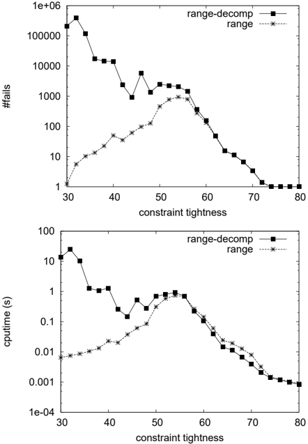
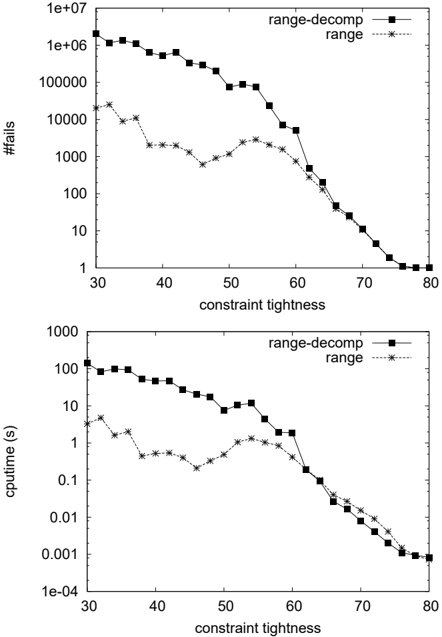
The purpose of this subsection is to compare the decomposition of Uses using Range constraints against a simple decomposition using more elementary constraints. We chose the Uses constraint because it is NP-hard to achieve GAC on the Uses constraint (see Section 6.1.4) and there is no propagator available for this constraint in the literature. Furthermore, one of the time-tabling problems at the University of Montpellier can easily be modelled as a CSP with Uses constraints. We first compare the two decompositions of Uses (with or without Range ) in terms of run-time as well as pruning power on random CSPs. Then, we solve the problem of building the set of courses in the Master of Computer Science at the University of Montpellier with the two decompositions.

7.2.1 Random CSPs

In order to isolate the effect of the Range constraint from other modelling issues, we used the following protocol: we randomly generated instances of binary CSPs and we added Uses ([ X 1 , .., X n ] , [ Y 1 , .., Y n ]) constraints. In all our experiments, we encode Uses in two different ways:

[range] : by decomposing Uses using Range as described in Section 6.1.4,

[decomp] : by decomposing the Uses constraint using primitive constraints as described next.

The problem instances are generated according to model B in [23], and can be described with the following parameters: the number of X and Y variables nx and ny in Uses constraints, the total number of variables nz , the domain size d , the number of binary constraint m 1 , the number of forbidden tuples t per binary constraint, and the number of Uses constraints m 2 . Note that the Uses constraints can have overlapping or disjoint scopes of variables. We distinguish the two cases. All reported results are averages on 1000 instances.

Our first experiment studies the effectiveness of decomposing Uses with Range for propagation alone (not solving). We compared the number of values removed by propagation on the models obtained by representing Uses constraints in two different ways, either using Range ( range ) or using the simple decomposition ( decomp ). To simulate what happens inside a backtrack search, we repeatedly and randomly choose a variable, assign it to one of its values and propagate the set of random binary constraints. After doing so for a given number of variables, if the CSP is still consistent, we enforce HC on each one of the two decompositions above. Hence, in the experiments, the constraints are exposed to a wide range of different variable domains. We report the ratio of values removed by propagation on the following classes of problems:

class A : 〈 nx = 5 , ny = 10 , nz = 35 , d = 20 , m 1 = 70 , t = 150 , m 2 = 3 ( overlap ) 〉 class B : 〈 nx = 5 , ny = 10 , nz = 45 , d = 20 , m 1 = 90 , t = 150 , m 2 = 3 ( disjoint ) 〉

in which the number of assigned variables varies between 1 and 14. A failure detected by the propagation algorithm yields a ratio of 1 (all values are removed).

We observe in Figures 4 and 5 that propagating the Uses constraint using the Range constraint ( range model) is much more effective than propagating it using the decomposition using elementary constraints ( decomp model). In certain cases, the range model more than doubles the amount of values pruned. For instance after 7 random assignments the decomp model prunes only 28.8% of the values for the first problem class (Fig. 4) and 4.4% for the second (Fig. 5) whilst the Range algorithm respectively prunes 56%

and 10.2% of the values. As we see in the next experiments, such a difference in pruning can map to considerable savings when solving a problem.

Our second experiment studies the efficiency of decomposing Uses with Range when solving the problems. Our solver used the smallest-domain-first variable ordering heuristic with the lexicographical value ordering and a cut-off at 600 seconds. We compared the cost of solving the two types of models: range and decomp . We report the number of fails and the cpu-time needed to find the first solution on the following classes of problems:

class C : 〈 nx = 5 , ny = 10 , nz = 25 , d = 10 , m 1 = 40 , t, m 2 = 2 〉

in which t varies between 30 and 80.

We observe in Figures 6 and 7 that using the decomposition using the elementary constraints ( decomp model) is not efficient (note the log scale). The instances solved here (classes C and D) are much smaller than those used for propagation (classes A and B). Solving larger instances was impractical. This second experiment shows that Range can reasonably solve problems containing Uses constraints. It also shows the clear benefit of using our algorithm in preference to the decomposition using elementary constraints over the under-constrained region. As the problems get over-constrained, the binary constraints dominate the pruning, and the algorithm has a slight overhead in run-time, pruning the same as the decomposition using elementary constraints.

7.2.2 Problem of the courses in the master of computer science

To confirm the results obtained on several types of random instances, we tackle the problem of deciding which courses to run in the Master of Computer Science at the University of Montpellier. This problem, which is usually solved by hand with the help of an Excel program, can be specified as follows. The second year of the Master of Computer Science advertises a set C of possible courses. There is a set L of n lecturers who have skills to teach some subset of the courses (between 1 and 9 per lecturer). There is a set S of m students who bid for which courses they would like to attend (between 6 and 10 bids per student). A course runs only if at least 5 students bid for it. Every lecturer participates in just one course, but several lecturers can be assigned to the same course. There is also a set P ⊆ L of professors who are in charge of the course in which they participate. The goal is to run enough courses so that all lecturers are assigned to

one course and all students can attend at least one of the courses for which they bid.

The models we used have variables L i representing which course is taught by lecturer i and variables S j representing one of the courses student j wants to attend. D ( L i ) contains all courses lecturer i can teach except those that received less than 5 bids. D ( S j ) contains all courses student j has bid for, except those that received less than 5 bids. We put a constraint Uses ([ L 1 , . . . , L n ] , [ S 1 , . . . , S m ]) and a constraint AllDifferent ( L i 1 , . . . , L i p ) where { L i 1 , . . . , L i p } = P . Model range decomposes Uses with Range , and model decomp decomposes Uses with primitive constraints as described in Section 7.2.1.

In the only instance we could obtain from the university, year-2008, there are 50 lecturers, 26 professors, 53 courses, and 177 students. We solved year-2008, both with model decomp and with model range . Both models could find a solution in a few milliseconds.

We modified the two models so that the satisfaction of the students is improved.

Instead of trying to satisfy only one of their choices, we try now to satisfy k choices. The models are modified in the following way. We create k copies of each variable S j , that is, S 1 j , S 2 j , . . . , S k j , with D ( S i j ) containing the same values as D ( S j ) (see above). We post constraints S 1 j < S 2 j < . . . < S k j that break symmetries and guarantee that S 1 j , S 2 j , . . . , S k j all take different values. Then, instead of having a single Uses constraint, we have k Uses constraints, one on each set S i 1 , S i 2 , . . . , S i m of variables: Uses ([ L 1 , . . . , L n ] , [ S 1 1 , . . . , S 1 m ]), . . . , Uses ([ L 1 , . . . , L n ] , [ S k 1 , . . . , S k m ]). Model range -k decomposes Uses with Range , and model decomp -k decomposes Uses with primitive constraints as described in Section 7.2.1.

We solved instance year-2008 with k = 2 , 3 , 4 , 5. When k = 2 or k = 3, both models find a solution in a few milliseconds, decomp -k being slightly faster than range -k . range -4 finds a solution in 4 fails and 5.83 sec. whereas decomp -4 was stopped after 24 hours without finding any solution. range -5 and decomp -5 were stopped after 24 hours without finding any solution or proving that none exists. This experiment shows that it can be effective to solve a real-world problem containing a global constraint like Uses by specifying it with Range instead of using a decomposition with elementary constraints.

7.3 Solving problems using Range and Roots

In Section 7.2.2, we showed how decomposing a global constraint with Range can be useful to solve a real-world problem. In this subsection we study another real-world problem that involves a greater variety of global constraints, some allowing decompositions with Range , some others with Roots . More importantly, we will compare monolithic propagators of existing well-known global constraints with their decompositions using Range and Roots . The purpose of this subsection is to see if solving real-world constraint problems using Range and Roots leads to acceptable performance compared to specialised global constraints and their propagators.

We used a model for the Mystery Shopper problem [16] due to Helmut Simonis that appears in CSPLib (prob004). We used the same problem instances as in [10] but perform a more thorough and extensive analysis. We partition the constraints of this problem into three groups:

• Temporal and geographical: All visits for any week are made by different shoppers. Similarly, a particular area cannot be visited more than once by the same shopper.
• Shopper: Each shopper makes exactly the required number of visits.
• Saleslady: A saleslady must be visited by some shoppers from at least 2 different groups (the shoppers are partitioned into groups).

The first group of constraints can be modelled by using AllDifferent constraints [25], the second can be modelled by Gcc [26] and the third by Among constraints [4]. We experimented with several models using Ilog Solver where these constraints are either implemented as their Ilog Solver primitives (respectively, IloAllDiff , IloDistribute , and a decomposition using IloSum on Boolean variables) or as their decompositions with Range and Roots . The decomposition of Among ([ X 1 , .., X n ] , [ d 1 , .., d m ] , N ) we use is the one presented in [6], that is, ( B i = 1 ↔ X i ∈ [ d 1 , .., d m ]) , ∀ i ∈ 1 ..n ∧ ∑ i B i = N . Note that this decomposition of the Among constraint maintains GAC in theory [6]. This

decomposition can be implemented in many solvers using disjunctions of membership constraints: or ( notmember ( X i , [ d 1 , .., d m ]) , B i = 1) and or ( member ( X i , [ d 1 , .., d m ]) , B i = 0). Unfortunately, Ilog Solver does not appear to achieve GAC on such disjunctions of primitives because the negated membership constraint notmember ( X i , [ d 1 , .., d m ]) is activated only if X i is instantiated with a value in [ d 1 , .., d m ] whereas it should be as soon as D ( X i ) ⊆ [ d 1 , .., d m ].

We report results for the following representative models:

• Alld -Gcc -Sum uses only Ilog Solver primitives;
• Alld -Gcc -Roots where Among is encoded using Roots ;
• Alld -Roots -Sum where Gcc is encoded using Roots ;
• Range -Gcc -Sum where AllDifferent is encoded using Range ;
• Alld -Roots -Roots where Among and Gcc are encoded using Roots ;

Note that Among encoded as Roots uses the decomposition presented in Section 6.2.2, the Gcc uses the decomposition presented in Section 6.2.1, and AllDifferent uses the decomposition presented in Section 6.1.1.

We study the following important questions:

• How does the Roots decomposition of the Among constraint compare to the Sum decomposition in terms of pruning and run-times?
• Does the decomposition of Gcc using Roots lead to a reasonable and acceptable loss in performance?
• Does the decomposition of AllDifferent using Range lead to a reasonable and acceptable loss in performance?
• Do we gain in performance by branching on the set variables introduced by the Roots decomposition?

To answer the first question, we will compare the model Alld -Gcc -Sum against the model Alld -Gcc -Roots . To answer the second question, we will compare the model Alld -Gcc -Sum against the model Alld -Roots -Sum . To answer the third question, we will compare the model Alld -Gcc -Sum against the model Range -Gcc -Sum . To answer the fourth question, we will compare Alld -Gcc -Sum against the model Alld -Roots -Roots that branches on the set variables.

The instances we use in the experiments are generated as follows. For each number of salesladies s ∈ { 10 , 15 , 20 , 25 , 30 , 35 } , we generate /ceilingleft ( s + 2 / 4) ∗ 4 /ceilingright shoppers, 4 visits. Furthermore, to determine the partitioning of the outlets, we bound the number of salesladies per outlet between a lower bound and an upper bound and generate all possible partitions within these bounds. The number of instances for each class is as follows; for 10 salesladies we have 10 instances, for 15 salesladies we have 52 instances, for 20 salesladies we have 35 instances, for 25 salesladies we have 20 instances, for 30 salesladies we have 10 instances, and for 35 salesladies we have 56 instances.

We also tested two variable and value ordering heuristics:

Table 1: The sum decomposition of Among in the Mystery Shopper problem versus the Roots decomposition using lex as a branching strategy.

	alld-gcc-sum-lex					alld-gcc-roots-lex
Size	#solved	time (sec.)		#fails		#solved	time (sec.)		#fails
		by self	by all	by self	by all		by self	by all	by self	by all
10	9	0.01	0.01	0.89	0.89	9	0.01	0.01	0.89	0.89
15	29	0.07	0.07	431.55	431.55	29	0.07	0.07	281.90	281.90
20	25	0.02	0.02	10.60	10.60	25	0.02	0.02	9.48	9.48
25	16	0.03	0.03	7.06	7.06	16	0.04	0.04	7.00	7.00
30	6	0.05	0.05	50.00	50.00	6	0.07	0.07	49.67	49.67
35	31	0.23	0.23	414.68	414.68	31	0.24	0.24	269.32	269.32

• We branch on the variables with the minimum domain first and assign values lexicographically. We refer to this as dom ;
• We assign a shopper to each saleslady for the first, then for the second week and so on. This a static variables and value ordering heuristic. We refer to this as lex .

However, since lex was consistently better than dom we only report the results using lex .

All instances solved in the experiments use a time limit of 5 minutes. For each class of instances we report the number of instances solved ( #solved ), the average cpu-time in seconds over all instances solved by the method ( by self ), the average cpu-time in seconds over all instances solved by both methods ( by all ), the average number of failures over all instances solved by the method ( by self ), the average number of failures over all instances solved by both methods ( by all ).

7.3.1 Among

When branching on the integer variables using lex (Table 1) strategy, the Alld -Gcc -Roots model tends to perform better than the Alld -Gcc -Sum model in terms of pruning (smaller number of fails). Note that the Sum decomposition misses some pruning because of the Ilog Solver propagators used in this decomposition, as explained at the beginning of Section 7.3. This explains the discrepancy. Both models solve the same number of instances. The results show that in this case of the Among constraint, our Roots decomposition is as efficient as the decomposition using elementary Sum constraints. Minor run-time differences are probably due to the cheaper propagator of Ilog Solver which achieves less pruning.

7.3.2 Gcc

The Gcc constraint is one of the most efficient and effective global constraints available in most constraint toolkits. The results comparing the Alld -Gcc -Sum model versus its equivalent (the Alld -Roots -Sum model) where instead of Gcc constraints we use our decomposition using Roots are shown in Table 2. We observe that when branching on the integer variables using lex , the loss in terms of pruning due to our decomposition is very low: the difference in number of fails is less than 5% on the hardest instances. This means that our decomposition should scale well when size and difficulty of problems

Table 2: The Gcc constraints in the Mystery Shopper problem versus the Roots decomposition using lex as a branching strategy.

	alld-gcc-sum-lex					alld-roots-sum-lex
Size	#solved	time (sec.)		#fails		#solved	time (sec.)		#fails
		by self	by all	by self	by all		by self	by all	by self	by all
10	9	0.01	0.01	0.89	0.89	9	0.01	0.01	1.78	1.78
15	29	0.07	0.07	431.55	431.55	29	0.43	0.43	434.38	434.38
20	25	0.02	0.02	10.60	10.60	25	0.10	0.10	10.60	10.60
25	16	0.03	0.03	7.06	7.06	16	0.23	0.23	38.31	38.31
30	6	0.05	0.05	50.00	50.00	6	0.43	0.43	72.33	72.33
35	31	0.23	0.27	414.68	505.48	23	3.89	3.89	521.74	521.74

Table 3: The AllDifferent constraints in the Mystery Shopper problem versus the Range decomposition using lex as a branching strategy.

	alld-gcc-sum-lex					range-gcc-sum-lex
Size	#solved	time (sec.)		#fails		#solved	time (sec.)		#fails
		by self	by all	by self	by all		by self	by all	by self	by all
10	9	0.01	0.01	0.89	0.89	9	0.02	0.02	0.89	0.89
15	29	0.07	0.07	431.55	431.55	29	0.18	0.18	431.55	431.55
20	25	0.02	0.02	10.60	10.60	25	0.17	0.17	10.60	10.60
25	16	0.03	0.03	7.06	7.06	16	0.32	0.32	7.06	7.06
30	6	0.05	0.05	50.00	50.00	6	0.57	0.57	50.00	50.00
35	31	0.23	0.23	414.68	414.68	31	1.39	1.39	414.68	414.68

increases. The difference in run-times is larger (up to more than one order of magnitude). This can be explained in part by the propagation algorithms for Range and Roots that we have implemented in Ilog Solver. They are far from being optimised, as opposed to the highly specialised native Gcc propagator. Overall, the loss appears to be acceptable. Our results show that, for the Gcc constraint, the decomposition into Roots leads to adequate performance for prototyping. Nevertheless, providing more efficient propagators for Roots is an interesting and open issue.

7.3.3 Alldifferent

The AllDifferent constraint is again one of the most efficient and effective global constraints available in most constraint toolkits. The results comparing the Alld -Gcc -Sum model versus its equivalent (the Range -Gcc -Sum model) where instead of AllDifferent constraints we use our decomposition using Range are shown in Table 3. We observe that when branching on the integer variables using lex both methods achieve the same amount of pruning even if we are not in a case where AllDifferent constraints are Permutation constraints (see Section 6.1.1). This means that even when our decomposition using Range theoretically hinders propagation, it can in practice achieve GAC. Concerning run-time efficiency, we observe that both methods solve the same number of instances. This is probably a consequence of the good level of pruning achieved by the decomposition of AllDifferent using Range . But the Alld -Gcc -Sum model is usually faster, up to one order of magnitude in the extreme case. Again, this can be explained in part by our basic implementation of the Range and Roots propagators in Ilog Solver, as opposed to the highly specialised native AllDifferent propagator.

Table 4: Branching on set variables in the Mystery Shoppers Problem

	alld-gcc-sum-lex					alld-roots-roots-set
Size	#solved	time (sec.)		#fails		#solved	time (sec.)		#fails
		by self	by all	by self	by all		by self	by all	by self	by all
10	9	0.01	0.01	0.89	0.89	10	0.05	0.05	98.20	91.33
15	29	0.07	0.07	431.55	431.55	52	0.12	0.05	102.83	23.34
20	25	0.02	0.02	10.60	10.60	35	1.30	1.25	852.14	794.20
25	16	0.03	0.03	7.06	7.06	20	5.08	5.12	2218.00	2170.12
30	6	0.05	0.05	50.00	50.00	10	15.05	3.65	4476.40	1675.33
35	31	0.23	0.23	414.68	412.24	51	33.88	35.86	6111.67	6410.14

7.3.4 Exploiting the set variables

In the previous subsections, we have seen that decomposing global constraints with Range and Roots constraints is a viable approach. Such decompositions generally give very small (if any) loss in terms of pruning and they give acceptable run-time performance. However, we have seen that our basic decomposition using Roots can be slow compared to highly specialised propagators such as those used by Ilog Solver for the Gcc constraint. In this subsection, we show that, even without optimising our code, we can improve the run-time performance of our decomposition just by exploiting its internal structure through the extra variables it introduces.

The decomposition of global constraints using Range and Roots introduces extra set variables. We here explore the possibility of branching on the set variables as follows. We branch on the set variables first, then on the integer variables with min domain once all set variables are instantiated. We refer to this as set . We compare the best model that uses the available constraints in Ilog Solver (model Alld -Gcc -Sum ) versus the best model that branches on the set variables (model Alld -Roots -Roots , in which the Among and the Gcc constraints are expressed using the Roots constraint). Surprisingly, we solve significantly more instances when branching on the set variables than the model Alld -Gcc -Sum . But, again, Alld -Gcc -Sum is a more efficient model when it manages to solve the instance.

These results are primarily due to the better branching strategy. However, such a strategy would not be easily implementable without Roots since the extra set variables are part of it. We observe here that the extra set variables introduced by the Roots decomposition may provide new possibilities for branching strategies that might be beneficial in practice.

These results show that by simply changing the branching strategy so that it exploits the internal structure of the decompositions, we obtain a significant increase in performance. This gain compensates the loss in cpu-time caused by the preliminary nature of our implementation.

8 Conclusion

We have proposed two global constraints useful in specifying many counting and occurrence constraints: the Range constraint which computes the range of values used by a set of variables, and the Roots constraint which computes the variables in a set

mapping onto particular values. These two constraints capture the notion of image and domain of a function, making them easy to understand to the non expert in constraint programming. We have shown that these two constraints can easily specify counting and occurrence constraints. For example, the open versions of some well-known global constraints can be specified with Range and Roots . Beyond counting and occurrence constraints, we have shown that the expressive power of Range and Roots allows them to specify many other constraints.

We have proposed propagation algorithms for these two constraints. Hence, any global constraint specified using Range and Roots can be propagated. In some cases, this gives a propagation algorithm which achieves GAC on the original global constraint (e.g. the Permutation and Among constraints). In other cases, this propagation algorithm may not make the original constraint GAC, but achieving GAC is NP-hard (e.g. the NValue and Common constraints). Decomposition is then one method to obtain a polynomial algorithm. In the remaining cases, the propagation algorithm may not make the constraint GAC, although specialised propagation algorithms can do so in polynomial time (e.g. the SymAllDiff constraint). Our method can still be attractive in this last case as it provides a generic means of propagation for counting and occurrence constraints when specialised algorithms have not yet been proposed or are not available in the constraint toolkit.

We have presented a comprehensive study of the Range constraint. We proposed an algorithm for enforcing hybrid consistency on Range . We also have presented a comprehensive study of the Roots constraint. We proved that propagating completely the Roots constraint is intractable in general. We therefore proposed a decomposition to propagate it partially. This decomposition achieves hybrid consistency on the Roots constraint under some simple conditions often met in practice. In addition, enforcing bound consistency on the decomposition achieves bound consistency on the Roots constraint whatever conditions hold.

Our experiments show the benefit we can obtain by incorporating the Range and the Roots constraints in a constraint toolkit. First, despite being intractable, the Roots constraint can be propagated using the decomposition we presented. Even if this decomposition hinders propagation in theory, our experiments show that it is seldom the case in practice. Second, in the absence of specialised propagation algorithms, Range and Roots appear to be a simple and a reasonable method for propagating (possibly intractable) global constraints that is competitive to other decompositions into more elementary constraints. Our experiments show that sometimes we do better than these other decompositions either in terms of pruning or in solution time or both (like the case of the decomposition of the Uses constraint). In addition, compared to highly specialised propagation algorithms like those for the AllDifferent and Gcc constraints in Ilog Solver, the loss in performance when using Range and Roots was not great. Thus, if the constraint toolkit lacks a specialised propagation algorithm, Range and Roots offer a quick, easy, and acceptable way of propagation. Finally, we observed that the extra set variables introduced in Range and Roots decompositions can be exploited in the design of new branching strategies. These extra set variables may provide both a modelling and solving advantage to the user. We hope that by presenting these results, developers of the many different constraint toolkits will be encouraged to include the Range and Roots constraints into their solvers.

Acknowledgements

We thank Eric Bourreau for having provided the data for the problem of the master of computer science of the university of Montpellier. We also thank our reviewers for their helpful comments which improved this paper.

References

1. R.K. Ahuja, T.L. Magnanti, and J.B. Orlin. Network flows . Prentice Hall, Upper Saddle River NJ, 1993.
2. N. Beldiceanu. Global constraints as graph properties on a structured network of elementary constraints of the same type. Technical report, Swedish Institute of Computer Science, 2000. SICS Technical Report T2000/01.
3. N. Beldiceanu. Pruning for the minimum constraint family and for the number of distinct values constraint family. In T. Walsh, editor, CP , volume 2239 of Lecture Notes in Computer Science , pages 211-224. Springer, 2001.
4. N. Beldiceanu and E. Contejean. Introducing global constraints in CHIP. Mathl. Comput. Modelling , 20:97-123, no. 12 1994.
5. N. Beldiceanu, I. Katriel, and S. Thiel. Filtering algorithms for the same and usedby constraints. In MPI Technical Report MPI-I-2004-1-001 , 2004.
6. C. Bessiere, E. Hebrard, B. Hnich, Z. Kiziltan, and T. Walsh. Among, common and disjoint constraints. In B. Hnich, M. Carlsson, F. Fages, and F. Rossi, editors, CSCLP , volume 3978 of Lecture Notes in Computer Science , pages 29-43. Springer, 2005.
7. C. Bessiere, E. Hebrard, B. Hnich, Z. Kiziltan, and T. Walsh. Filtering algorithms for the NVALUE constraint. Constraints , 11(4):271-293, 2006.
8. C. Bessiere, E. Hebrard, B. Hnich, Z. Kiziltan, and T. Walsh. Filtering algorithms for the NVALUE constraint. In R. Bartak and M. Milano, editors, CPAIOR , volume 3524 of Lecture Notes in Computer Science , pages 79-93. Springer, 2005.
9. C. Bessiere, E. Hebrard, B. Hnich, Z. Kiziltan, and T. Walsh. The RANGE and ROOTS constraints: some applications. Technical report COMIC-2006-003, 2006.
10. C. Bessiere, E. Hebrard, B. Hnich, Z. Kiziltan, and T. Walsh. The RANGE and ROOTS constraints: Specifying counting and occurrence problems. In L.P. Kaelbling and A. Saffiotti, editors, IJCAI , pages 60-65. Professional Book Center, 2005.
11. C. Bessiere, E. Hebrard, B. Hnich, Z. Kiziltan, and T. Walsh. The RANGE constraint: Algorithms and implementation. In J.C. Beck and B.M. Smith, editors, CPAIOR , volume 3990 of Lecture Notes in Computer Science , pages 59-73. Springer, 2006.

1. C. Bessiere, E. Hebrard, B. Hnich, Z. Kiziltan, and T. Walsh. The ROOTS constraint. In F. Benhamou, editor, CP , volume 4204 of Lecture Notes in Computer Science , pages 75-90. Springer, 2006.
2. C. Bessiere, E. Hebrard, B. Hnich, and T. Walsh. The complexity of global constraints. In D.L. McGuinness and G. Ferguson, editors, AAAI , pages 112-117. AAAI Press / The MIT Press, 2004.
3. C. Bessiere, E. Hebrard, B. Hnich, and T. Walsh. The complexity of reasoning with global constraints. Constraints , 12(2):239-259, 2007.
4. C. Bessiere, E. Hebrard, B. Hnich, and T. Walsh. The tractability of global constraints. In M. Wallace, editor, CP , volume 3258 of Lecture Notes in Computer Science , pages 716-720. Springer, 2004.
5. B.M.W. Cheng, K.M.F. Choi, J.H.M. Lee, and J.C.K. Wu. Increasing constraint propagation by redundant modeling: an experience report. Constraints , 4(2):167192, 1999.
6. R. Debruyne and C. Bessiere. Some practicable filtering techniques for the constraint satisfaction problem. In IJCAI , pages 412-417, 1997.
7. B. Hnich, Z. Kiziltan, and T. Walsh. Modelling a balanced academic curriculum problem. In CPAIOR , pages 121-131, 2002.
8. ILOG. Reference and User Manual . ILOG Solver 5.3, ILOG S.A., 2002.
9. F. Laburthe. Choco: implementing a CP kernel. In Proceedings of TRICS: Techniques foR Implementing Constraint programming Systems, a post-conference workshop of CP , Singapore, 2000.
10. M. Maher. Analysis of a global contiguity constraint. In Proceedings of the Workshop on Rule Based Constraint Reasoning and Programming, held alongside CP , Ithaca NY, 2002.
11. F. Pachet and P. Roy. Automatic generation of music programs. In J. Jaffar, editor, CP , volume 1713 of Lecture Notes in Computer Science , pages 331-345. Springer, 1999.
12. P. Prosser. An empirical study of phase transitions in binary constraint satisfaction problems. Artif. Intell. , 81(1-2):81-109, 1996.
13. C.G. Quimper, A. L´ opez-Ortiz, P. van Beek, and A. Golynski. Improved algorithms for the global cardinality constraint. In M. Wallace, editor, CP , volume 3258 of Lecture Notes in Computer Science , pages 542-556. Springer, 2004.
14. J.C. R´ egin. A filtering algorithm for constraints of difference in csps. In AAAI , pages 362-367, 1994.
15. J.C. R´ egin. Generalized arc consistency for global cardinality constraint. In AAAI/IAAI, Vol. 1 , pages 209-215, 1996.

1. J.C. R´ egin. The symmetric alldiff constraint. In T. Dean, editor, IJCAI , pages 420-425. Morgan Kaufmann, 1999.
2. F. Rossi, P. van Beek, and T. Walsh. Handbook of Constraint Programming , Elsevier, 2006.
3. A. Schrijver. Combinatorial Optimization -Polyhedra and Efficiency . SpringerVerlag, Berlin, 2003.
4. C. Schulte and P.J. Stuckey. Speeding up constraint propagation. In M. Wallace, editor, CP , volume 3258 of Lecture Notes in Computer Science , pages 619-633. Springer, 2004.
5. P. Van Hentenryck and J.P. Carillon. Generality versus specificity: An experience with ai and or techniques. In AAAI , pages 660-664, 1988.
6. P. Van Hentenryck and Y. Deville. The cardinality operator: A new logical connective for constraint logic programming. In ICLP , pages 745-759, 1991.
7. P. Van Hentenryck, Y. Deville, and C.M. Teng. A generic arc-consistency algorithm and its specializations. Artif. Intell. , 57(2-3):291-321, 1992.
8. W.J. van Hoeve and J.C. R´ egin. Open constraints in a closed world. In J.C. Beck and B.M. Smith, editors, CPAIOR , volume 3990 of Lecture Notes in Computer Science , pages 244-257. Springer, 2006.