Redundant Sudoku Rules

BART DEMOEN

Department of Computer Science, KU Leuven, Belgium [email protected]

MARIA GARCIA DE LA BANDA

Faculty of Information Technology, Monash University, Australia [email protected] submitted 15 February 2012; revised 17 July 2012; accepted 17 July 2012

Abstract

The rules of Sudoku are often specified using twenty seven all different constraints, referred to as the big constraints. Using graphical proofs and exploratory logic programming, the following main and new result is obtained: many subsets of six of these big constraints are redundant (i.e., they are entailed by the remaining twenty one constraints), and six is maximal (i.e., removing more than six constraints is not possible while maintaining equivalence). The corresponding result for binary inequality constraints, referred to as the small constraints, is stated as a conjecture.

KEYWORDS : Sudoku, all different constraints, inequalities, maximal redundancy

1 Introduction

On the 18th of May 2008, the following question was posted on rec.puzzles : 'what's the minimum amount of checking that needs to be done to show that a completed 9x9 grid is valid?'. We prove that the short answer is: '21 all different constraints'. The complete answer shown here is the result of a set of theorems whose proofs are presented in an intuitive graphical representation, together with a set of Prolog programs 1 whose help was welcome for guiding our intuition and for dealing with some of the combinatorial explosion resulting from the symmetries of the Sudoku puzzle.

A very common formulation of the Sudoku (Wikipedia ; Jussien 2007) puzzle is as follows: each 3 × 3 box, as well as each row and each column, must contain all the numbers from 1 to 9. As a constraint satisfaction problem (CSP), the Sudoku puzzle can be modeled using a set of 81 variables x ij , one per row i ∈ [1 .. 9] and column j ∈ [1 .. 9], 81 domain constraints indicating that the domain of each x ij is [1..9], and 27 all different constraints with 9 variables each (9 constraints for

1 The relevant programs are available at http://people.cs.kuleuven.be/bart.demoen/sudokutplp. We have used different Prolog systems, including SICStus Prolog, B-Prolog and hProlog. These programs run in other systems with little change.

the variables in each of the rows, another 9 for each of the columns, and a final 9 for each of the boxes). We refer to these 27 constraints as the big constraints and use the word Sudoku in italics to denote the associated CSP model, i.e., the one containing all 27 big constraints together with the 81 domain constraints.

/negationslash

/negationslash

/negationslash

An all different constraint can also be formulated as the pairwise binary inequality constraints of its input variables. For example, all different ( { y 1 , y 2 , y 3 } ) is logically equivalent to the conjunction of the constraints y 1 = y 2 , y 1 = y 3 , and y 2 = y 3 . We refer to these binary =-constraints as the small constraints . When Sudoku is modeled using small constraints, it is easy to see that each cell is involved in 20 small constraints: 8 in the same box, 6 in the same row and 6 in the same column. Since there are 81 cells, and each constraint is posted twice, there are in total 810 different small constraints (as opposed to 27 big ones). Whenever a CSP model M specified using (big or small) constraints, together with the 81 domain constraints, is equivalent to Sudoku (i.e., it has the same set of solutions), we say M is Sudoku .

/negationslash

It was always intuitively clear to us that some of the small constraints must be redundant , i.e., entailed by the others. However, the questions 'which and what is the size of the largest redundant set of small constraints?' remained to be answered. The situation was even worse for big constraints: when we started this research, it was not even clear to us whether any single big constraint is redundant. Both issues are attacked here: we give a complete answer for the big constraints and a partial answer for the small constraints.

We begin by recalling some common Sudoku-related terminology in Section 2. Section 3 introduces our graphical representation of Sudoku modeled with big constraints. This representation significantly simplifies the reasoning required for showing that some sets of big constraints with six or less elements are redundant (Section 4). We then describe a Prolog program that systematically applies these two positive lemmas to find all sets of redundant big constraints with six or less elements (Section 5). While doing this, we discover seven negative lemmas (Section 5.1). The combination of positive and negative lemmas results in a complete classification of all sets of 21 (27 - 6) big constraints (Section 5.2). We then turn to the study of sets of seven big constraints and show that none of them are redundant (Section 5.3). As before, our Prolog program discovers a new negative lemma, whose proof is also presented graphically. We then show that at least 20% of the small constraints can be redundant (Section 6), and conjecture that no more is possible. Finally, in Section 7 we conclude and discuss related work and possible extensions.

2 Terminology

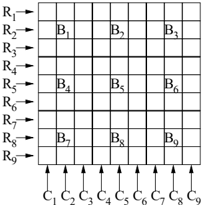
The 27 big constraints in Sudoku correspond to the 27 regions in which its board is usually divided (see the attached picture): the 9 rows, 9 columns and 9 boxes, whose big constraints will be denoted as R 1 , . . . , R 9 , as C 1 , . . . , C 9 , and as B 1 , . . . , B 9 , respectively. We use the word horizontal (vertical) chute to refer to three horizontal (vertical) boxes.

1

For instance, the boxes associated to constraints B 2 , B 5 , and B 8 denote a vertical chute.

As mentioned before, we are interested in exploring Sudoku models where some big constraints are missing. In the following, we will use Missing ( n ) to denote the set of Sudoku models that have 27 -n big constraints. For example, every model in Missing (5) has 22 big constraints (plus, of course, the usual 81 domain constraints).

3 A graphical Representation of Sets of Big constraints

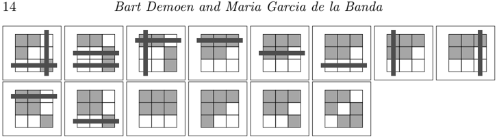
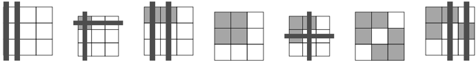
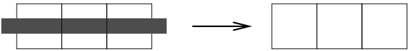
The standard set notation is not visually clear once the number of elements in the set is high. Since we will be dealing mostly with sets of more than 20 big constraints, we have developed a graphical representation of the Sudoku model that we find more useful. This graphical representation always shows the borders of the boxes of a Sudoku board and assumes all 81 domain constraints are specified in the model. Further, all 27 big constraints are also specified unless they are explicitly represented as missing in the figure. A column, row or box constraint is represented as missing if it is shaded. Figure 1 shows an example.

The pictures provide a quick and intuitive view into which big constraints are present in the model and which are not. Note that the absence of a big constraint does not mean it is violated, simply that it has not been specified in the associated model.

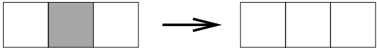
Using the same idea, we can represent a set of big constraints applicable only to a chute (any chute): this is illustrated in Figure 2.

4 Two Constructive Lemmas

Let us now prove two positive lemmas, i.e., how a subset of the big constraints can be shown to entail another big constraint.

4 Bart Demoen and Maria Garcia de la Banda

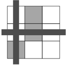
Lemma 4.1

The conjunction of the big constraints in { R 1 , R 2 , R 3 , B 1 , B 3 } entails B 2 . This is represented graphically by means of the following picture:

Proof Let us fill the chute with 27 numbers, so that the constraints in are satisfied. To do so, let us try to place any value N ∈ 1 .. 9 in the chute. Since R 1 , R 2 and R 3 are present, there must be exactly one N in each row, which means there must be three N s in the chute. Since B 1 and B 3 are also present, exactly one of these three N s must be in box 1 and exactly another one in box 3. This leaves exactly one (the third) N in box 2. Since this holds for any N ∈ 1 .. 9 , B 2 also holds.

The dual of Lemma 4.1 is Lemma 4.2.

Lemma 4.2

Proof Let us fill the chute with 27 numbers, so that the constraints in are satisfied. To do so, let us again try to place any value N ∈ 1 .. 9 in the chute. Since B 1 , B 2 and B 3 are present, there must be exactly one N in each box, which means there must be three N s in the chute. Since R 1 and R 3 are also present, exactly one of these three N s must be in row 1 and exactly another one in row 3. This leaves exactly one (the third) N in row 2. As before, this means R 2 also holds.

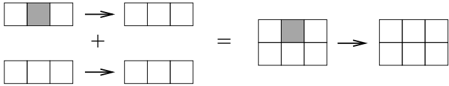
From now on we assume the graphical representation is clear enough not to require accompanying text. Together with the trivial lemma , the above two lemmas form the building blocks of a corollary and of a whole set of theorems: we simply glue several applications of these lemmas to form a new one, as exemplified in the following picture:

+

=

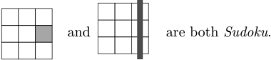
We are now ready for our corollary:

Corollary 4.3

and

are both Sudoku .

Proof Glue together twice the trivial lemma with Lemma 4.1 and Lemma 4.2, respectively, and obtain the result immediately.

Taking into account the symmetries of the puzzle, it follows that every single big constraint is (by itself) redundant, i.e., that every model in Missing (1) is Sudoku ! We will see later that this is not true for any other Missing ( n ) with n > 1.

Note that the two lemmas really are constructive , i.e., they show how to infer one new big constraint from a set of big constraints. The following two theorems exploit that constructive power to reason further about redundancy.

.

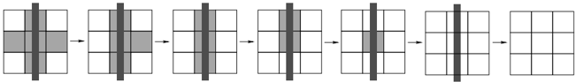
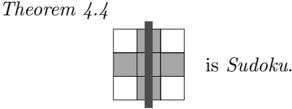
Theorem 4.5

Proof We prove this by repeatedly using Lemma 4.2 as follows:

Each of the two theorems above shows a model in Missing (6) that is Sudoku . While there are many symmetric versions of these theorems, we have chosen those that are visually most pleasing to us. The next section fully classifies Missing (6).

5 A Full Classification of Missing (6)

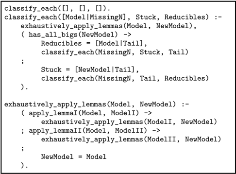
Lemmas 4.1 and 4.2 allow us to add a new big constraint to a set of big constraints while retaining equivalence, as shown in the proof of Theorem 4.4. We use this to implement a Prolog program that attempts to classify all models in Missing (6) as either Sudoku or not, and whose simplified form is shown Figure 3. Intuitively, the program receives as input in MissingN a list with all models in Missing ( n ), for some particular n . Then, for each model Model of MissingN , it exhaustively applies lemmas 4.1 and 4.2 computing the (possibly reduced) model in NewModel . If NewModel contains the 27 big constraints (and, thus, it is Sudoku ) it adds Model to the Reducible list and, otherwise, it adds NewModel to the list Stuck of models with less than 27 big constraints at which it got stuck. These latter models need special attention.

While the number of models in Missing (6) is relatively small (296,010), we can

further reduce it by eliminating the spatially symmetric models. We have run 2 the complete Program I over the (reduced) set of Missing ( n ) for n = 6 (from which we can also derive the results for n = [2 .. 5]). Surprisingly, the program only failed to prove equivalence to Sudoku for the following models:

Note that while the last two are models in Missing (6), the others (from right to left) are models in Missing (5) , Missing (4) , Missing (3), and Missing (2), which were obtained during the proving process by applying Lemma 4.1 or 4.2 to some model in Missing (6). As we prove in the next section, none of these seven models is Sudoku and, thus, none of the models in Missing (6) whose proof got stuck is Sudoku either. This is because if a model M in Missing ( n ) is not Sudoku , then any model M ′ in Missing ( n ′ ) where n ′ > n and the constraints in M ′ are a subset of those in M , cannot be Sudoku either.

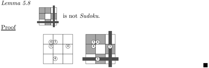
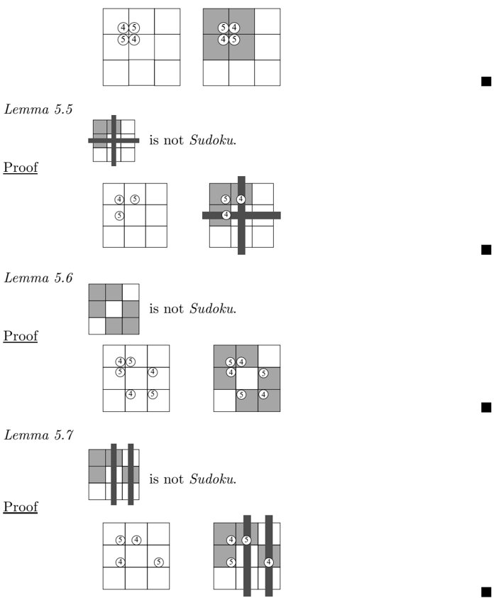
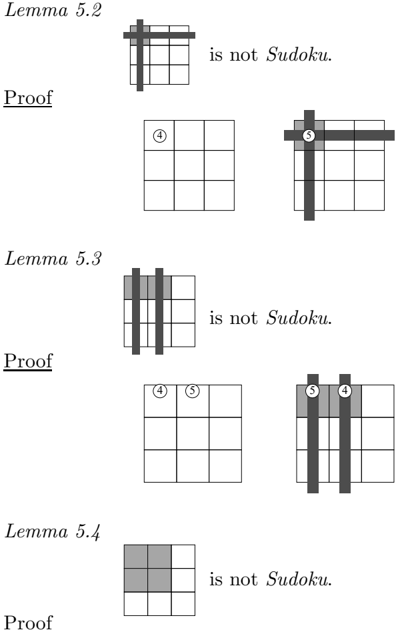
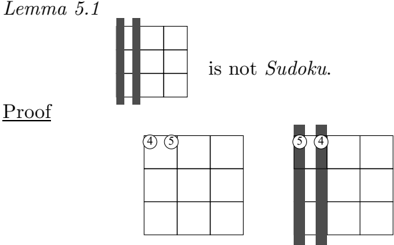
5.1 Seven Negative Lemmas

We proceed by proving seven negative lemmas, stating that each of the seven models shown above is not Sudoku . The proof to each lemma consists of two pictures: the left picture represents a solution to the Sudoku puzzle where the circled cells have the specified 4 or 5 value (note that there might be many solutions that satisfy this). For example, in the first lemma, the left picture represents any solution where cell x 11 has value 4 and cell x 13 has value 5. The right picture in a proof represents

2 See file classify.pl at the already mentioned website: the actual Prolog code has an extra argument collecting the models shown in Appendix II

the result of changing every circled 4 in the left picture by a circled 5, and vice versa. In all cases the result is a non-solution (to Sudoku ) with the violated big constraints depicted as shaded. These violated constraints are exactly those that, if removed, the lemma claims cannot yield Sudoku . Since the picture proves that if the big constraints in question are removed the non-solution is accepted as a solution, the lemma is proved.

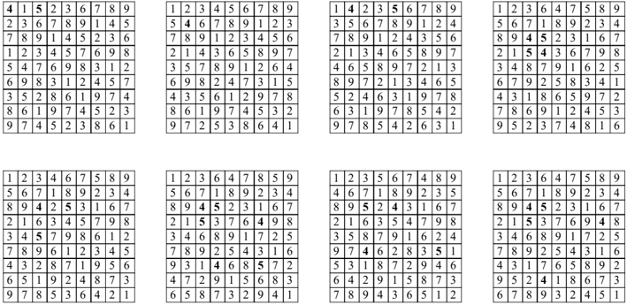
The other six negative lemmas follow the same schema. We expect readers to work out the details for them after convincing themselves that such an initial solution exists for each proof (some such solutions are provided in Appendix III).

The above positive and negative lemmas give us a complete method for determining whether any model in Missing (6) is Sudoku or not: if the application of the constructive lemmas results in Sudoku , then the model is Sudoku ; otherwise it will get stuck in one of the seven negative models and, thus, is known not to be Sudoku . In this sense, the two constructive lemmas are complete (and also confluent). This can be used to render our first program more useful by changing the classify each/3 predicate to also check whether the models who do not have all 27 big constraints are one of the seven negative lemmas. If so, it ignores them, otherwise, as before, it adds them to Stuck . Note that, for the case of Missing (6), Stuck is then empty. We refer to the modified version of Program I by Program II, and we have further

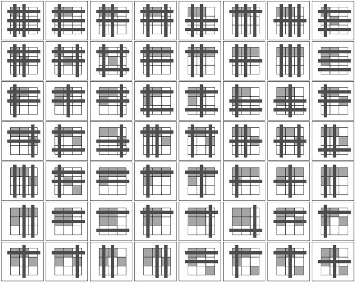
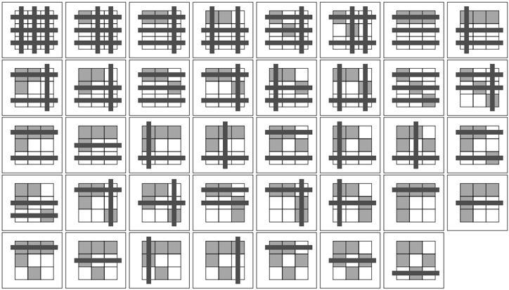
modified it to generate the pictures 3 that can be found in the appendices I and II: we run this modified program with n = 6 and, for each model in (the reduced) Missing (6) a picture is output. Interestingly, there are 39 different models in (the symmetry reduced) Missing (6) that are Sudoku , and 70 that are not.

5.3 No Model in Missing (7) is Sudoku

When we run Program II with n = 7, every model gets stuck either in one of the previous seven lemmas, or in a model with a new set of big constraints. This model results in one more negative lemma, which is not implied by any of the previous negative lemmas.

Readers can easily check that none of the models in Lemma 5.1 up to Lemma 5.7 is contained in the above model. As a result, no model in Missing (7) is Sudoku . Or put otherwise: no redundant set of big constraints has more than six elements.

5.4 Generalizing to Puzzles of Size N

Our techniques can be readily applied to the investigation of Sudoku puzzles of different sizes. Up to now, we have dealt with puzzles of size 3, i.e., there are 3 4 cells, in a 3 2 by 3 2 board, with 3 2 rows, columns and boxes. Clearly, Lemmas 4.1 and 4.2 generalize easily to other sizes. For example, for size 4, one just needs to add one non-shaded block constraint to the pictures to ensure the lemmas remain true.

This suggests that for size n , no model in Missing (2 ∗ n +1) is Sudoku . Proving this is, however, outside the scope of the current paper.

6 Redundancy for the Small Constraints

For each of the models in Missing (6) one can easily count the number of different small constraints it represents: for the ones that are Sudoku , the highest count is 690, and the lowest count is 648. This lowest count occurs only for the set of Theorem 4.5, and we denote the model with this set of small constraints by Small 4 . 5 .

It seems worth trying to remove small constraints from Small 4 . 5 and check

3 See file genfigs.pl at the website.

try_each_inequality(Model):remove(X#\=Y,Model,Rest), (gordonRoyle(Givens), solve([X#=Y|Rest],Givens) -> writeln(is_not_Sudoku(Rest)) ; writeln(maybe_Sudoku(Rest)) ).

whether the resulting model is still Sudoku . To achieve this, we have implemented a Prolog program 4 that selects every small constraint x = y in Small 4 . 5 , creates a new set Rest = Small 4 . 5 \ { x = y } , and then tries to prove Rest is not Sudoku by posting all constraints in Rest plus constraint x = y to a constraint solver and running the solver on a set of Sudoku puzzles. If a solution is found, then Rest cannot be Sudoku , since x cannot be equal to y in it. Note that this is similar to our manual treatment of the set of models classified as stuck by Program I, where each model is proved not to be Sudoku by finding a solution to the model that is not a solution of Sudoku . The (simplified) Prolog program is provided in Figure 4. The set of Sudoku puzzles we have used comes from Gordon Royle's website (Royle ) and consists of more than 50,000 minimal Sudoku puzzles each containing 17 given entries: their minimality was proven recently in (McGuire et al. 2012). We refer to this set as GR .

/negationslash

Interestingly, the above program determines that every strict subset Rest of Small 4 . 5 is not Sudoku : for each Rest , there is indeed a puzzle in GR which has a solution that makes the two variables in the removed inequality equal. This proves that the set Small 4 . 5 forms a locally minimal set of small constraints for Sudoku . This was independently verified (Codish 2012) by running a CNF-encoding of that statement using the BEE-compiler described in (Metodi and Codish 2012). Moreover, using the same technology, we were jointly able to prove that each of the 39 models M of Missing (6) that are Sudoku (see Appendix I) has the following property:

M has a subset of inequalities of size 648 that is Sudoku and is also a locally minimal set of small constraints

We were not able to reduce those M 's any further, i.e., beyond 648. Although these results do not allow us to conclude that Sudoku models with a smaller set of small constraints are not possible, we dare to conjecture the following:

Conjecture: No model with less than 648 small constraints is Sudoku .

7 Discussion and Conclusion

The message in rec.puzzles mentioned in the introduction also refers essentially to our Corollary 4.3, i.e., that in every chute, one row (or column) constraint needs no

4 See file sudoku648.pl at the website.

/negationslash

checking, if the other constraints in that chute are validated. 5 Clearly, other people have wondered about redundant big constraints in Sudoku, and our main result many sets of six big constraints are redundant - often surprises people. It is all the more interesting that the popular (Ist et al. 2006) refers to the 'minimal encoding' as one containing all big rules: our results clearly indicate that such encoding is not minimal at all. Further, while redundant rules can strengthen propagation and, thus, reduce the search space, it has already been noted (Kwon and Jain 2006) that the classical Conjunctive Normal Form encodings for Sudoku in SAT generate too many redundant clauses, and compact encodings (which eliminate redundant clauses) are more efficient. Our work can be used to inform such encodings.

Our conjecture that no model with less than 648 small constraints is Sudoku remains to be proven. While the combinatorial challenge is great, we are currently investigating the use of unavoidable sets as in (McGuire et al. 2012). We have also obtained a full classification of models that use small constraints for the more restricted problem of Latin Squares (Demoen and Garcia de la Banda ).

Apart from our novel results themselves, and the use of exploratory (Constraint) Logic Programming, this paper also introduces a powerful graphical representation of sets of constraints that renders the proofs easy to understand, and that can be re-used for larger Sudoku puzzles.

Exploratory programming was essential in this research: it helped us discover potential theorems and lemmas which we subsequently turned into hard general proofs. Further, the use of Prolog has been critical: as it can be seen from the website, the programs are small, fast, easy to read and modify. This would have been very difficult without the combined power of backtracking (for almost everything, particularly finding all solutions satisfying a set of conditions), constraint solving (to easily define Sudoku and test the satisfiability of many of its subsets) and logic variables (to easily identify and access the variables in the model).

/negationslash

/negationslash

/negationslash

Redundant constraints are very often good for the performance of CP systems, and indeed, all solvers we checked perform much slower (about a factor 2000) with a minimal set of big constraints. So it might seem counterproductive to try to find redundant constraints if the aim is to remove them. However, our work gives some insight into the construction of new (redundant) inequality constraints: while deriving new equalities from a set of equalities is easy because equality is transitive, this does not hold for inequalities. The difficulty and possibility of deriving new inequalities depends crucially on the domains of the variables. For instance, from a chain of inequalities x 1 = x 2 = . . . = x n between boolean variables, one may conclude that x 1 = x 4 (amongst others), but if the domains have a larger cardinality, this is no longer true. Since our work provides a complete set of rewrite rules on sets of all different constraints (together with the domain constraints) for a particular CSP, it forms a first step in the development of a more general inequality inference framework.

/negationslash

Finally, note that our result on big constraints completes in some sense the result

5 At the time of that post, we had already completed our classification of the big constraints.

in (McGuire et al. 2012): 17 clues is necessary, and so are 21 big constraints. It would be interesting to have the corresponding result for small constraints.

Acknowledgements The main results reported here were obtained while the first author was on a research visit at Monash University in April 2008, and enjoying the Stuckey hospitality in Apollo Bay and Elwood, Australia. Many thanks for a most enjoyable stay. We are grateful to Michael Codish for his help with obtaining some of the results related to the conjecture. This research was partly sponsored by he Australian Research Council grant DP110102258, by the Brussels-Capital Region through project ParAps, and by the Research Foundation Flanders (FWO) through projects WOG: Declarative Methods in Computer Science and G.0221.07 .

References

• Codish, M. 2012. Private communication.
• Demoen, B. and Garcia de la Banda, M. Maximal sets of redundant constraints in latin square. Forthcoming. Tech. rep.
• Ist, I. L. , Lynce, I. , and Ouaknine, J. 2006. Sudoku as a SAT problem. In Proceedings of the 9 th International Symposium on Artificial Intelligence and Mathematics, AIMATH 2006, Fort Lauderdale . Springer.
• Jussien, N. 2007. A to Z of SUDOKU . ISTE, London.
• Kwon, G. and Jain, H. 2006. Optimized CNF encoding for Sudoku puzzles. 13th International Conference on Logic for Programming Artificial Intelligence and Reasoning, LPAR 2006 - short paper.
• McGuire, G. , Tugemann, B. , and Civario, G. 2012. There is no 16-clue Sudoku: Solving the Sudoku minimum number of clues problem. CoRR abs/1201.0749 .
• Metodi, A. and Codish, M. 2012. Compiling finite domain constraints to SAT with bee (version with appendix). Tech. rep., Ben-Gurion University, Department of Computer Science. Accepted as full paper for ICLP 2012.
• Royle, G. Minimum Sudoku. http://people.csse.uwa.edu.au/gordon/sudokumin.php. Wikipedia . Sudoku. http://en.wikipedia.org/wiki/Sudoku.

Appendix III: Initial solved puzzles for Lemma 5.1 up to Lemma 5.8