Reinforcement Learning Based on Active Learning Method

Hesam Sagha 1 , Saeed Bagheri Shouraki 2 , Hosein Khasteh 1 , Ali Akbar Kiaei

1 1 ACECR, Nasir Branch, Tehran, Iran 2 Department of Electrical Engineering Sharif University of Technology,Tehran, Iran [email protected], [email protected], [email protected], [email protected]

Abstract

In this paper, a new reinforcement learning approach is proposed which is based on a powerful concept named Active Learning Method (ALM) in modeling. ALM expresses any multi-input-single-output system as a fuzzy combination of some single-input-singleoutput systems. The proposed method is an actor-critic system similar to Generalized Approximate Reasoning based Intelligent Control (GARIC) structure to adapt the ALM by delayed reinforcement signals. Our system uses Temporal Difference (TD) learning to model the behavior of useful actions of a control system. The goodness of an action is modeled on Reward-Penalty-Plane. IDS planes will be updated according to this plane. It is shown that the system can learn with a predefined fuzzy system or without it (through random actions).

1. Introduction

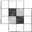
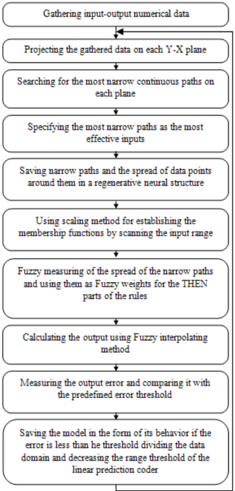
ALM [1,2,3,4] is a recursive fuzzy algorithm, which expresses a multi-input-single-output system as a fuzzy combination of several single-input-single-output systems. It models the input-output relations for each input and combines these models to find out the overall system model. ALM starts with gathering data and projecting them on different data planes. The horizontal axis of each data plane is one of the inputs and the vertical axis is the output. IDS processing engine will look for a behavior curve, hereafter narrow line, on each data plane. If the spread of data over the narrow line is more than a threshold, data domains will be divided and the algorithm runs again. The heart of this learning algorithm is a fuzzy interpolation method which is used to derive a smooth curve among data points. It is done by applying a three-dimensional membership function to each data point, which expresses the belief for the data point and its neighbors. Each data point is considered as a source of light, which has a pyramid-shape illumination pattern. As the vertical distance from this source of light increases, its illuminating pattern will interfere with its neighbors forming new bright areas. The projection of the process on the plane is called IDS.

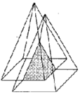
As it is shown in Fig 2, we can use a pyramid as a three dimensional fuzzy membership function of a data point and its neighboring points. By applying IDS method to each data plane, two different types of information will be extracted. One is the narrow path and the other is the deviation of the data points around each narrow path. Each narrow path shows the behavior of output relative to an input; and spread of the data points around this path shows the importance degree of that input in overall system behavior. Less deviation of data points around the path represents a higher degree of importance and vice versa.

Sagha et al [5] proposed a method which combines genetic algorithm and IDS to obtain better partitions over input variables. Their method is called GIDS (Genetic IDS).

Shahdi et al [6] proposed RIDS method that replaces each two consequent points with their midpoint instead of applying a 2-d fuzzy membership function on each data. RIDS converges to the center of gravity of data and increases the number of points in order to keep data expansion in plane. In addition, they proposed another method called (Modified RIDS ) MRIDS that support negative data points. In MRIDS, if two consequent points are positive, the result is similar to that of RIDS and the replacing point is their midpoint. Nevertheless, if one of the points is negative, then the replacing point is a point located near the positive point on the line which connects two points; so negative point has an effect of deviating center of gravity from positive points.

MRIDS considers that the rewards and punishments are accessible after each action, but when they are delayed and this delay is not determined, it will not converge correctly.

Here we used another method called Reinforcement ALM ( RALM ), to add reinforcement capability to the algorithm. We used the concepts of Action Selection

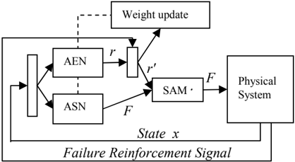
Network ( ASN ), Action Evaluation Network ( AEN ), and Stochastic Action Modifier ( SAM ) that are proposed in GARIC [7] as an actor-critic algorithm.

GARIC: The architecture of GARIC is schematically shown in Fig 3. ASN maps a state vector into a recommended action, F , using fuzzy inference. AEN maps a state vector and a failure signal into a scalar score that indicates state goodness. This is also used to produce internal reinforcement, r' . AEN can be a neural network structure or a fuzzy system [8] or alike. SAM uses both F and r' to produce an action F' , which will be applied to the plant. Learning occurs by fine-tuning the parameters in the two networks: in the AEN , the weights or fuzzy parameters are adjusted; in the ASN , the pa-

rameters describing the fuzzy membership functions are changed. These are done by gradient descent approach. AEN parameters are updated via Temporal Difference Learning method.

Temporal Difference Learning: is a prediction method. It approximates its current estimate based on previously learned estimates by assuming subsequent predictions are often correlated in some sense. A prediction is made, and when the observarion is availabe the prediction is adjusted to better match the observation. If each state st has the prediction value v(st ) that denotes the goodness of done actions in that state, then the updating formula is:

where α t is learning rate and δ is a constant in the range of [0,1] and R t+1 is the received reward at time t+1.[9]

2. Proposed Method

In our method we used a similar structure to GARIC . ASN is an IDS fuzzy system. AEN is made up of a plane called Reward-Penalty-Plane ( RPP ). On this plane is the information of how much the done action in a specific state is good. From control viewpoint, this plane can be called Error-Change in Error-Plane because one axis

Tetha

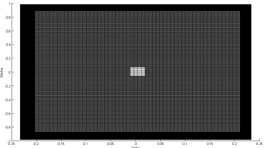
Figure 4 . Initial Reward-Penalty Plane for an inverse pendulum system. Middle points denote the desired states (-0.012R< θ <0.012 R and -0.05R/s < ∆θ < 0.05R/s) and have the maximum value (1), margin points denote penalty areas and have the negative minimum value (less than zero, more than -1), and other points are in the play area.

denotes error and the other denotes cha the value of each point in this plane much we can trust the selected action specific state. SAM changes the value output by considering the output of AEN an action is SAM changes it less. RPP i up of the desired variable to control. A three regions on RPP plane, i) reward sired area we like the controller takes th This area has the fixed value of one . ii consists of states that are not desirabl makes it unstable. The value of this are lowest negative value. iii) Play area rest of the surface that has the value of z initial plane is shown in figure 4, for a s stable the variable angle . anging error, and shows that how n of ASN in that of fuzzy system N . More relevant s a surface made At first we have d area : is the dehe state into that. i) Penalty area : le in system and ea is stuck to the : this area is the zero initially. An system we like to

During the run when data is availab RPP in the previous time step and its approach to the value of RPP in the c and its neighbors as same as TD(0). ble, the value of s neighbors will current time step

(

(

RPP e t

-

where, delta is the value of changing error of control variable at time t , ce is c and win is the IDS window shows neighbors must be effected and it can Gaussian window with the center value When an action is rewarded the rate of u but when an action is penalized, λ is ve cause we assumed the number of false more than true actions for a system. RPP , e(t) is the changing in error how much the n be a pyramid, e of one or alike. update, λ , is high, ery low. It is beactions is much

After updating the RPP plane, we m planes for the previous action and its n case, we reward the action if it goes to punish it when it goes to worse state. Th of an action will be obtained by avera values: must update IDS neighbors. In this o better state and he total goodness aging over delta

where ini is the i th input variable.

Fuzzy system can be adapted onlin after spreading each datum and neglect ative areas of IDS planes, narrow lines fuzzy inference system are updated. To action (step time t ) after fuzzy inferen ASN , for exploration and exploitation i change the obtained value by following ne. In this case, ting data in negs of a predefined o select the next nce procedure in in the space, we g formula:

where N(0,Var) is a normally distr able with variance Var and α is a c gives the best score for an action action of ASN will be applied witho ributed random variconstant. When RPP (i.e. 1), the selected out manipulation.

For offline learning, after some d the RPP plane converges and no ch or a specific number of iteration is planes that has both positive and n ative areas show that the actions w this part of space transform the syst Therefore, by neglecting the data in filter bad actions. Finally, by estim and using ALM , we can construct th data capturing, when hanges occurred in it, s passed, we get IDS egative values. Negwhich are chosen in tem into worse state. n these areas, we can mating narrow lines, he fuzzy system.

Another problem exists when th of reward area. If we use the orig system, we have vibrations in this the learning system is not learned state is in reward area. To handle th fuzzy scaling. In this kind of scalin variable of fuzzy system will be sca reward range/input range: e state is in the range inal generated fuzzy range. It is because how to act when the his problem we used ng, the range of input aled proportion to the

' ( ( i i i In In Range Reward In = × where In i is i th input which is a part )) / ( ) i i Range In (6) t of RPP .

Output range will be scaled by

( ( ( )) i Max Range Reward In / ( )) i Range In (7)

Therefore, we do not need another fu variables must be scaled and use the system. uzzy system; just generated fuzzy

This approach has some advantage with MRIDS , especially when the probl reach into a desired state. Also we expl reward and penalty areas and there is n how and on what trajectory the system goal. s in comparison lem has delays to licitly define the no need to define m can reach the

3. Results

We modeled the well-known inv problem with two input, theta, θ , and (Dtheta), θ . Reward area was chose [-0.23, 0.23] radian and θ = [-0.98, 0. penalty areas are when each variable is input range. λ is chosen to be 0.9 for r for penalties. Penalty areas are set to be was chosen to be 0.021. verse pendulum angular velocity en between θ = 98] radian/s and more than 0.9 of ewards and 0.05 e -0.5. Time step

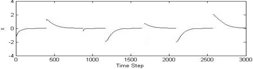
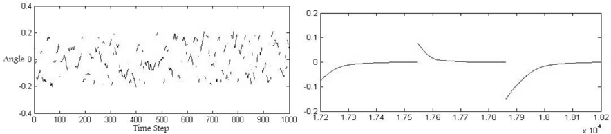
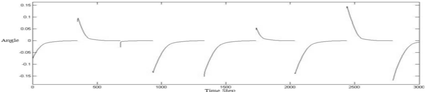
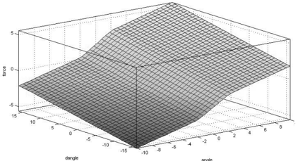
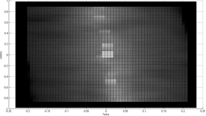
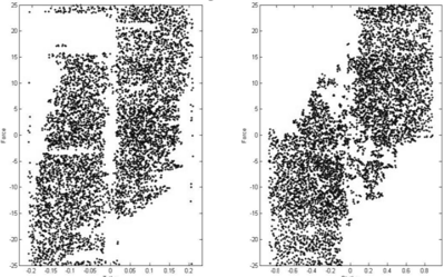
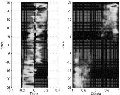
We used two methods of action sele ginning of run. The first one used ran stead of a predefined fuzzy system, so by formula (5) was needed. After 2000 only 32 successes during it, we got which are shown in Fig. 5. Success is w state is in the reward area. White areas dark areas are negative. Figure 6 shows extracted from all data after removing b located on negative part of IDS plane ward-Penalty Plane is shown in Fig. 7 ALM, we got a fuzzy system with only surface of input-output-force is shown shows some random initial states and th to the desired point. Rise time is 2.71 a %0.0. The second method uses an inco tem in ASN with four rules. After ab steps of online learning, the system lear Fig 10 shows first 1000 time steps and Learning by GARIC takes about 10000 in our system it takes less than 20000 ti ection in the bendom actions inno manipulation 00 sequences and the IDS planes when the system are positive and s the data that are bad ones that are s. The final Re7. After applying y four rules. The in Fig. 8. Fig. 9 heir convergence and overshoot is orrect fuzzy sysbout 18000 time rned to be stable. d last 1000 ones. 00 time steps but ime steps.

In addition, we modeled ball and be assumed the system has three inputs, θ outputs x and v . θ is the angle of beam line passing through the origin, r0 is th the distance of ball from the origin. v0 is of ball's speed and r and v are the final v and speed. Our goal is to move the ball zero, so we define the RPP with respec control it, we have two inputs v0 and x0 θ . eam system. It is θ , x 0, v 0 and two m with horizontal he initial value of s the initial value values of distance into the position ct to x and v . To 0 and one output

The results of RALM for some ran shown in Fig. 11. Generated fuzzy s rules. The rise time is 1.6 s and overshoo ndom inputs are system has four ot is %0.0. Table

1 shows the result of other proposed ALM and FALCON. It can be se reduced about 13% of supervised shoot is detected. d algorithm based on een that rise time is ALM and no over-

4. Conclusion

ALM is a powerful idea for mod to support reinforcement learning. another plane to get the informati signals. The approach is useful whe idea about the goodness of an act wards and penalties must be cons siders these very well. deling. We changed it . Our approach uses ion of reinforcement en there is no explicit ion, and delayed residered. RALM con-

Results show that RALM learn proposed ALM based algorithms. ns better than other

Table 1. Comparing control par ling method rameters of 4 controld

	Fuzzy rules	Over- shoot	Rise time
FALCON-ART	28	23.5%	2.11
Unsupervised ALM	4	14.3%	1.87
Supervised ALM	4	0	1.85
RALM	4	0	1.61

alfue

Figure 8. Fuzzy syste em surface

5. References

1. S.Bagheri, G.Yuasa, N.Honda, 'Fuzzy by an active Learning Method', 31 st Sympos Control, SIC 98 Controller Design sium of Intelligent
2. S.Bagheri, N.Honda,'Hardware Simu Learning Process', 15 th Fuzzy Symposium , O ulation of Brain Osaka, June 99.
3. S.Bagheri, N.Honda, 'A New Method and Saving Fuzzy Membership Functions' posium , Toyama, 1997. d for Establishing ', 13 th Fuzzy sym-
4. S.Bagheri, N.Honda, 'Outlines of a S Brain Simulation', Methodologies for the C And Application of Soft Computing, IIZUK , oft Computer For Conception, Design 1998
5. H.Sagha, S. B. Shouraki, M.Dehghani, ' Spread', International Symposium in Intell Technology Application, IITA, China,2008 'Genetic Ink Drop ligent Information
6. A.Shahdi, S.Bagheri, 'Supervised Act thod as an intelligent linguistic Controller Implementation', IASTED , Spain, 2002 ive Learning Meand Its Hardware
7. H.Berenji, P.Khedkar, 'Learning and Tu Controllers Through Reinforcement', IEE Neural Network , Vol 3, No 5, 1992. uning Fuzzy Logic EE Transaction on
8. H.Berenji, P.Khedkar, 'Using Fuzzy L mance Evaluation in Reinforcem NASA-TM-111486 Logic For Performent Learning',
9. R. Sutton,A. Barto. Reinforcement Lea 1998 arning. MIT Press,

Time

Figure10. Online learning; L Left: First 1000 time steps, Right: Time steps between 172 00 and 18200