Representing and Solving Asymmetric Bayesian Decision Problems

Thomas D. Nielsen

Finn V. Jensen

Department of Computer Science Aalborg University

Fredrik Bajers Vej 7C, DK-9220 Aalborg 0, Denmark

Abstract

This paper deals with the representation and solution of asymmetric Bayesian decision problems. We present a formal framework, termed asymmetric influence diagrams, that is based on the influence diagram and al­ lows an efficient representation of asymmet­ ric decision problems. As opposed to exist­ ing frameworks, the asymmetric influence di­ agram primarily encodes asymmetry at the qualitative level and it can therefore be read directly from the model.

We give an algorithm for solving asymmetric influence diagrams. The algorithm initially decomposes the asymmetric decision problem into a structure of symmetric subproblems organized as a tree. A solution to the de­ cision problem can then be found by propa­ gating from the leaves towards the root using existing evaluation methods to solve the sub­ problems.

1 INTRODUCTION

The power of an influence diagram, both as an analysis tool and a communication tool, lies in its ability to con­ cisely and precisely describe the structure of a decision problem[Smith et al., 1993]. However, influence dia­ grams can not efficiently represent the so-called asym­ metric decision problems; decision problems are usu­ ally asymmetric in the sense that the set of possible outcomes of a chance variable may vary depending on the conditioning states, and the set of legitimate deci­ sion options of a decision variable may vary depending on the different information states [Qi et al., 1994].

Various frameworks have been proposed as alterna­ tives to the influence diagram when dealing with asym­ metric decision problems. [Covaliu and Oliver, 1995]

extends the influence diagram with another diagram, termed a sequential decision diagram, which describes the asymmetric structure of the problem as comple­ mentary to the influence diagram which is used for specifying the probability model. [Smith et al., 1993] introduces the notion of distribution trees within the framework of influence diagrams. The use of distribu­ tion trees allows the possible outcomes of an observa­ tion to be specified, as well as the legitimate decision options of a decision variable. However, as the distri­ bution trees are not part of the influence diagram, the structure of the decision problem can not be deduced directly from the model. Moreover, the sequence of decisions and observations is predetermined, i.e., pre­ vious observations and decisions can not influence the temporal order of future observations and decisions. Finally, distribution trees have a tendency of creating large conditionals during the evaluation since they en­ code both numeric information and information about asymmetry. To overcome this problem [Shenoy, 2000] presents the asymmetric valuation network as an ex­ tension of the valuation network for modelling sym­ metric decision problems[Shenoy, 1992]. The asym­ metric valuation network uses indicator functions to encode asymmetry, thereby separating it from the numeric information. However, asymmetry is still not represented directly in the model and, as in [Smith et al., 1993], the sequence of observations and decisions is predetermined.1

In this paper we present the asymmetric influ­ ence diagram which is a framework for represent­ ing asymmetric decision problems. The asymmet­ ric influence diagram is based on the partial influ­ ence diag ra m [Nielsen and Jensen, 1999b], and encodes structural asymmetry at the qualitative level; struc­ tural asymmetry has to do with the occurrence of vari­ ables in different scenarios as opposed to functional asymmetry which has to do with the possible out-

1 Further details and comparisons of these methods can be found in [Bielza and Shenoy, 1999].

comes/decision options of the variables. As a mod­ elling language, the syntactical rules of the asymmet­ ric influence diagram allow decision problems to be described in an easy and concise manner. Further­ more, its semantic specification supports an efficient evaluation algorithm.

An outline of this paper is as follows. In Section 2 we describe the partial influence diagram, together with the terms and notation used throughout this pa­ per. In Section 3 we formally introduce the asym­ metric influence diagram and illustrate this framework by modelling a highly asymmetric decision problem termed "the dating problem". Finally, in Section 4 we present an algorithm for solving asymmetric influence diagrams.

2 PRELIMINARIES

The partial influence diagram (PID) was defined in [Nielsen and Jensen, 1999b] as an influence diagram (ID) with only a partial temporal order over the deci­ sion nodes. That is, a PID is a directed acyclic graph I = (U, £), where the nodes U can be partitioned into three disjoint subsets; chance nodes Uc, decision nodes U0 and value nodes Uv. The chance nodes (drawn as circles) correspond to chance variables, and represent events which are not under the direct control of the de­ cision maker. The decision nodes (drawn as squares) correspond to decision variables and represent actions under the direct control of the decision maker. We will use the concept of node and variable interchangeably if this does not introduce any inconsistency, and we assume that no barren nodes are specified by the PID since they have no impact on the decisions.2

With each chance variable and decision variable X we associate a finite discrete state space W x which de­ notes the set of possible outcomes/ decision options for X. For a set U' of variables we define the state space as Wu, = x{WxiX E U'}.

The set of value nodes (drawn as diamonds) defines a set of utility potentials with the restriction that value nodes have no descendants. Each utility potential in­ dicates the local utility for a given configuration of the variables in its domain; the domain of a utility poten­ tialljJx, for a value node X, is denoted dom(ljJx) = nx, where nx is the immediate predecessors of X. The to­ tal utility is the sum or the product of the local utilities (see [Tatman and Shachter, 1990]); in the remainder of this paper we assume that the total utility is the sum of the local utilities.

2 A chance node or a decision node is said to be barren if it does not precede any other node, or if all its descendants are barren.

The uncertainty associated with a variable X E Uc is represented by a conditional probability potential <Px = P(XInx) : W x unx --t [0; 1]. The domain of a conditional probability potential <Px is denoted dom(<J:>xl ={X}unx.

The arcs in a PID can be partitioned into three dis­ joint subsets, corresponding to the type of node they go into. Arcs into value nodes represent functional dependencies by indicating the domain of the associ­ ated utility potential. Arcs into chance nodes, denoted dependency arcs, represent probabilistic dependencies, whereas arcs into decision nodes, denoted informa­ tional arcs, imply information precedence; if D E U0 and (X , D) E £ then the state of X is known when decision D is made.

The set of informational arcs induces a partial order -< on Uc U U0 as defined by the transitive closure of the following relation:

• Y-< Di, if (Y, Dd is a directed arc in I (Di E Uo ).
• Di -< Y, if (Di, X,, Xz, . . . , Xm, Y) is a directed path in I (Y E Uc UU0 and DiE Uo).
• Di -< A, if A -/< Dj for all Di E U0 (A E Uc and DiE Uo).
• Di -< A, if A -/< Di and :3Di E U0 s.t. Di -< Di and A-< Di (A E Uc and DiE Uo).

In what follows we say that two different nodes X and Y are incompatible if X -/< Y and Y -/< X.

We define a realization of a PID I as an attachment of potentials to the appropriate variables in I, i.e., the chance nodes are associated with conditional probabil­ ity potentials and the value nodes are associated with utility potentials. So, a realization specifies the quan­ titative part of the model whereas the PID constitutes the qualitative part.

Evaluating a PID amounts to computing a strategy for the decisions involved. A strategy can be seen as a prescription of responses to earlier observations and decisions, and it is usually performed according to the maximum expected utility principle; the max­ imum expected utility principle states that we shall always choose a decision option that maximizes the expected utility. However, the strategy for a deci­ sion variable may depend on the variables observed thus, we define an admissible total order for a PID I to describe the relative temporal order of incompati­ ble variables: an admissible total order is a bijection 13 : Uo U Uc H {1, 2, ... , IUo U Ucl} s.t. if X -< Y then I3(X) < /3(Y), where-< is the partial order induced by I. In what follows < will be used to denote the total ordering 13 s.t. X< Y if P.,(X) < P.,(Y). Notice, that an

admissible total ordering of a PID I implies that I can be seen as an ID.

Given an admissible total ordering <, we define an admissible strategy relative to < as a set of functions �< = {&[310 E Uo }, where &[3 is a decision function given by:

and pred(D)< ={XIX< D} (the index< in pred(D)< will be omitted if this does not introduce any confu­ sion). Given a realization of a PID I, we term an ad­ missible strategy relative to <, an admissible optimal strategy relative to < if the strategy maximizes the ex­ pected utility for I; two admissible optimal strategies are said to be identical if they yield the same expected utility. A decision function &[3, contained in an ad­ missible optimal strategy relative to <, is said to be an optimal strategy for D relative to <. Note that an optimal strategy for a decision variable D relative to < does not necessarily depend on all the variables observed. Hence, we say that an observed variable X is required for D w.r.t. < if there is a realization of I s.t. the optimal strategy for D relative to < is a non-constant function over X. By this we mean that there exists a configuration y over dom(S[3)\{X} and two states x1 and xz of X s.t. S[3(x1, y) -1- S[3(xz, y).

Definition 1. A realization of a PID I is said to define a decision problem if all admissible optimal strategies for I are identical. A PID is said to define a decision problem if all its realizations define a decision problem.

The above definition characterizes the class of PIDs which can be considered welldefined since the set of admissible total orderings for a PID I corresponds to the set of legal elimination sequences for I. However, it also conveys the problem of only having a partial temporal ordering of the decision variables; the rela­ tive temporal order of a chance variable (eliminated by summation) and a decision variable (eliminated by maximization) may vary under different admissible or­ derings and summation and maximization does not in general commute. So, in order to determine whether or not a PID defines a decision problem we introduce the notion of a significant chance variable.

Definition 2. Let I be a PID and let A be a chance variable incompatible with a decision variable D in I. Then A is said to be significant for D if there is a realization and an admissible total order < for I s.t. :

• A occurs immediately before D under <.
• The optimal strategy for D relative to < is differ­ ent from the one achieved by permuting A and D in<.

Based on the above definition we have the following theorem which characterizes the constraints necessary and sufficient for a PID to define a decision problem.

Theorem 1 ([Nielsen and Jensen, 1999b]). The PID I defines a decision problem if and only if for each decision variable D there does not exist a chance variable A significant for D.

See [Nielsen and Jensen, 1999b] for a structural char­ acterization of the chance variables being significant for a given decision variable.

3 ASYMMETRIC INFLUENCE DIAGRAMS

[Qi et a!., 1994 ] states that decision problems are usu­ ally asymmetric in the sense that the set of possible outcomes of a chance variable may vary depending on the conditioning states, and the set of legitimate decision options of a decision variable may vary de­ pending on the different information states. Equiva­ lently, [Bielza and Shenoy, 1999] characterizes a deci­ sion problem as being asymmetric if, in its decision tree representation, the number of scenarios is less than the cardinality of the Cartesian product of the state spaces of all chance and decision variables. However, both of these characterizations fail to recognize deci­ sion problems in which the relative temporal order of two variables vary w.r.t. to previous observations and decisions; this is for example very common for trou­ bleshooting problems. Thus, we define an asymmetric decision problem as follows:

Definition 3. A decision problem is said to be asym­ metric if, in its decision tree representation, either:

• the number of scenarios is less than the cardinality of the Cartesian product of the state spaces of all chance and decision variables or
• there exists two scenarios in which the relative temporal order of two variables differ.

In order to deal with such asymmetric decision prob­ lems we introduce the asymmetric influence diagram (AID). An AID is a labeled directed graph I = (U, £,F), where the nodes U can be partitioned into four disjoint subsets; test-decision nodes (UT ) , action­ decision nodes (UA), chance nodes (Uc) and value nodes (Uv ) ; we will sometimes omit the distinction between test-decisions and action-decisions by simply referring to a node in Uo = UT UUA as a decision node.

The chance nodes and value nodes are similar to the chance nodes and value nodes in a PID. The deci­ sion nodes correspond to decision variables and rep­ resent actions under the direct control of the decision

maker. A test-decision (drawn as a triangle) is a de­ cision to look for more evidence, whereas an action­ decision (drawn as a rectangle) is a decision to change the state of the world.

The arcs £ in an AID can be partitioned into four dis­ joint subsets. An arc into a value node or a chance node is semanticly defined as in the PID framework if, in case of the latter, it does not emanate from a test-decision node. Arcs into decision nodes, termed informational arcs, imply a possible information prece­ dence; if there is an arc from a node X to a decision node 0 then the state of X may be known when de­ cision 0 is made. This redefinition is needed since we deal with asymmetric decision problems, i.e., the set of variables observed immediately before decision 0 is taken may dependent on previous decisions and observations.

If there exists an arc, termed a test arc, from a test­ decision node 0 to a chance node X, then the state of 0 determines whether or not X is eventually observed; having an arc from a test-decision node to a chance node represents a logical relation and does not imply probabilistic dependence. Note that in the trivial case, where X is observed no matter the state of 0, the arc (0, X) implies information precedence only. If there exists an arc (D, 0 1) from a test-decision node 0 to another decision node 01, then (0, 01) implies infor­ mation precedence ( ( 0, 0 1) is an informational arc) however, ( 0, 0 1) is termed a test arc if the state of 0 determines whether or not 0 1 is eventually decided upon; whether we are referring to an informational arc or a test arc is conveyed by the label associated with 0 1; in the remainder of this paper we let I denote the graph obtained from I by removing all test arcs and informational arcs.

The asymmetry of a decision problem is graphically represented in the AID by a set of restriction arcs and by a set of labels :F. The set of restriction arcs (drawn as dashed arcs) is a subset of the informational arcs. A restriction arc (X, 0) indicates that the set of legit­ imate decision options for 0 may vary depending on the state of X, in which case we say that X is restrictive w.r.t. 0 (or X is restricting 0). The set of labels :F is associated with a subset of the nodes and informa­ tional arcs. A label specifies under which conditions the associated node or informational arc occurs in the decision problem. The following rules informally sum­ marize the semantics of labels when specifying asym­ metry in the AID; in the remainder of this section they will be referred to as rule (i)-(iii), respectively:

1. Let X be a node labelled with fx and let Y be the variables observed before X is observed (or decided upon). If fx is unsatisfied w.r.t. the state configuration Y = y observed, then X is not in-

eluded in the scenario.

• ii) Let (X, 0) be an informational arc labeled with f(X,DJ and let Y be the variables observed be­ fore X is observed (or decided upon). If f(x,o) is unsatisfied w.r.t. the state configuration Y = y observed, then (X, D) is not included in the sce­ nario.
• iii) If there exists a directed path from a node X to a node Y in I, then whenever X is not included in the scenario Y is not included in the scenario either.

Based on the rules above we require that if the label of a node Z is a function of a node X, then there must exist an arc from X to Z (See Figure 1).

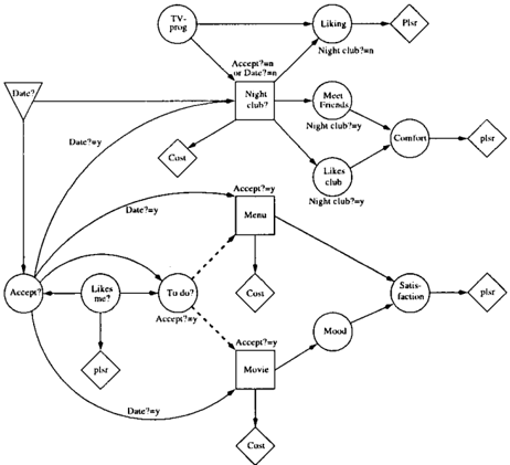
Example 1. [The dating problem] Joe has to de­ cide whether or not to ask a girl he has recently met on a date. If Joe decides not to ask her out he can choose either to stay at home and watch TV or visit a night club; before taking that decision Joe observes what programs will be on TV that night. The plea­ sure of staying at home is influenced by his liking of the program watched, whereas the pleasure of going to a night club is dependent on the comfort of going to that night club and the entrance fee; comfort is depen­ dent on whether Joe likes the night club and whether he meets any friends there.

If Joe decides to ask her out her response will depend on her feelings towards him. If she declines the date, Joe can decide to go to a night club or stay at home and watch TV; we assume that the two "staying at home scenarios" are the same. If she accepts to go on a date with him, Joe will ask her whether she wants to go to a restaurant or to the movies. The choice of movie (decided by Joe) may influence her mood which in turn may influence Joe's satisfaction concerning the evening. Similarly, the choice of menu (decided by Joe) might influence Joe's satisfaction.

This decision problem is represented by the AID de­ picted in Figure 2. The variable Date? is represented as a test-decision since it has no impact on the value of Accept?. In the evaluation of whether or not to ask for a date, the distribution of Accept? is relevant and Accept? is therefore always part of the entire decision problem.

The decision Night Club? is decided upon if Joe ini-

tially chooses not to ask the girl for a date; the label as­ sociated with Night Club? specifies a logical-or and is therefore satisfied by the state configuration Date?=n. If Joe chooses to go to a night club the chance vari­ ables Meet Friends and Likes Club influence Joe's com­ fort which in turn influences the pleasure of going to that club; the chance variable Liking is excluded from the decision problem since Liking is only included if Club?=n (rule (i)). Notice that this property could also be modelled by introducing a redundant state in the variable Liking. However, having redundant states tends to obscure the asymmetric structure of the de­ cision problem, and is in general computationally de­ manding.

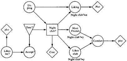
Since Date?=n the informational arcs from Accept? are excluded (rule (ii)) meaning that her potential re­ sponse is never observed; as previously mentioned, Ac­ cept? is still part of the decision problem as opposed to e.g. Liking if Club?=y. Now, as Accept? is never observed the va r iables only labeled by the state of Ac­ cept? are removed (rule (i)), together with all their successors (rule (iii)). The resulting decision problem is depicted in Figure 3; the variables Accept and Likes me? are included in the figure for the purpose of the AID being a tool for communication.

If Joe on the other hand chooses to ask the girl for a date he will observe her response (Accept?). If she declines the invitation he can choose either to go to a night club or stay at home. If she accepts the in­ vitation the variable To do? will be observed which can restrict the possible decision options for Menu and Movie.

There is a small technical problem with the variable

Satisfaction which has the mutually exclusive variables Menu and Movie as predecessors. As no descendant of an excluded variable can be included (rule (iii)), we would unintentionally exclude Satisfaction whenever Menu or Movie are included. This problem can be solved by duplicating Satisfaction and its descendants or by adding an extra state (no-decision) to the vari­ ables Menu and Movie. In order to minimize redun­ dancy in the representation we have chosen the latter.

D

3.1 THE QUALITATIVE LEVEL

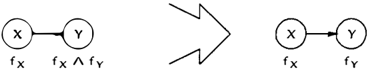
Now, from rule (iii) we can infer the following syn­ tactical simplification: If there exists a directed path from a node X to a node Y in I, then Y "inherits" the label associated with X, i.e., Y is "effectively" la­ beled with fx I\ fv, where fx and fv are the labels explicitly associated with X and Y, respectively. This means that we need not explicitly associate Y with the label fx I\ fv (see Figure 4a). The set of vari­ ables from which a chance variable X "inherits" labels is given by dep(X) = Y, where Y is the set of vari­ ables from which there exists a directed path to X in I; to ensure consistency it should be noted that de­ cision nodes, value nodes and informational arcs "in­ herit" labels from the empty set. E.g. in Figure 2 the variable Meet Friends is "effectively" conditioned on (Night club?=y I\ (Accept?=n V Date?=n)) since dep (Meet Friends) = Night club?.

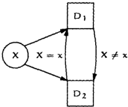
The AID allows the specification of directed cycles with the restriction that before any of the nodes in a cycle are observed the cycle must be "broken", i.e., no matter the variables observed there must exist at least one unsatisfied label associated with a node or an

informational arc in the cycle. This syntactical con­ straint compensates for the traditional constraint that the graph should be acyclic. Having cycles in an AID supports the specification of decisions for which the temporal order is dependent on previous observations and decisions. For instance, in Figure 5 decision Dz is taken before D 1 if X = x but D 1 is taken before D 2 if X =f. x.

Formally, a label is a Boolean function defined as a combination of Boolean variables, the constants true ( 1) and false ( 0) and the operators 1\ (conjunction), V (disjunction),--. (negation),=} (implication) and� ( bi-implication).

The Boolean variables are used to represent the con­ ditioning on states e.g. if a node Y is conditioned on X = x then X = x should be represented as a Boolean variable in the label associated with Y. However, for ease of notation we shall use e.g. X = x directly in the label (without creating an actual Boolean variable); a Boolean variable in the context of labels must there­ fore denote a state configuration of some node in the AID.

A truth assignment to a Boolean function f is the same as fixing a set of variables in the domain of f, i.e., if X = x represents a Boolean variable in the domain of f, then X = x can be assigned either true or false by associating X with some state x' E W x (denoted f[X H x']). E.g. (X = x)[X H x'] = 1 if x = x' and (X = x ) [ X H x'] = 0 otherwise.

[n the remainder of this paper, we assume that each 10de X is associated with a label fx, i.e., if X is not .ssociated with a label in I = (U, £,F), then we extend =-with the label fx = 1. Moreover, we will use dom(f) >denote the domain of the label f; the domain of a bel is the set of nodes referenced by the label.

chance variable X is said to be present in I given c:onfiguration c over a set of variables C, if ( fx 1\ 'Edep(X) fy )[C H c] = 1 in I given c. A chance vari­ e X is said to be unresolved in I given a configura1 c over a set of variables C if dom( fx [C H c]) =f. 0 fx[C H c] '/:. i(Vi E {0, 1}), or 3Y E dep(X) s.t. l(fv[C H c]) =f. 0 and fv[C H c] t i(Vi E {0, 1}).

The concepts present and unresolved are similarly de­ fined for value nodes, decision nodes and informational arcs.

3.2 THE QUANTITATIVE LEVEL

A decision variable D is associated with a set of re­ strictive functions; a restrictive function is given by y0 : Wn0 y 2Wo and specifies the legitimate deci­ sion options forD given a configuration of n0 � n�, where n� denotes the set of variables which can re­ strict the legitimate decision options for D. In Figure 2 the restrictive function associated with Movie specifies that the state no-decision is the only legitimate deci­ sion option if To do?=restaurant (similar for Menu if To do?=movie).

The uncertainty associated with a chance variable X is represented by a partial conditional probability po­ tential tPx = P(XIInx) : Wxun� Y [0; 1], where nx = n x \UT; by definition, a test-decision variable has no probabilistic influence on a chance variable. A partial probability potential can specify that given a configuration of the conditioning set for a chance vari­ able X, some states of X are impossible (denoted .L); we make a conceptual distinction between an impos­ sible state and a state having zero probability. Note that if all the states of X are impossible for some con­ figuration of the conditioning set, then this must be reflected in the labeling of X e.g. if P(XIY) is only de­ fined for Y = 1J, then Y = 1J must occur in the label of X.

A value node X is associated with a partial utility po­ tential1\>x : Wnx Y JR+ U {0}; requiring that the par­ tial utility potential does not take on negative values is not an actual restriction as any utility potential can be transformed s.t. it adheres to this assumption. Fur­ thermore, as for the PID we assume that the total utility is the sum of the local utilities.

The combination of partial potentials (addition, multi­ plication and division) is defined similarly to the com­ bination of total functions by treating the undefined value (.L) as an additive identity and a multiplica­ tive zero. In particular, this ensures consistency when defining the total utility as being the sum of the local utilities.

As for the PID we define a realization of an AID as an attachment of probability and utility potentials to the appropriate variables. The probability and utility potentials associated with an AID I is denoted ll>r and 'l'r, respectively. Given a realization ll>r U'Jlr of an AID I the set of probability potentials with X E X in the domain will be denoted ll>x, i.e., ll>x = {<P E ll>ri3X E X: X E dom(<jl)}.

3.3 SPLIT CONFIGURATIONS AND DECISIONS IN CONTEXT

When taking a decision in an asymmetric decision problem, previous observations and decisions may de­ termine the variables observed before the decision in question. For both semantic and computational rea­ sons it is important to identify the variables actually observed before taking a particular decision. For in­ stance, in the AID depicted in Figure 2 it would not be meaningful to have an optimal strategy for Menu con­ ditioned on both Date?=n and Accept?=y since this is an impossible state configuration. So, in order to reason about the different informational states when taking a decision D we must associate D with a con­ text describing the variables observed. That is, we need to identify the possible temporal orderings of the variables and in particular, the variables which influ­ ence the occurrence of future variables.

Definition 4. Let I be an AID and let :F be the set of labels associated with I. A variable X is said to be a split variable in I if there exists a label f E :F s.t. X E dom(f). The set of split variables in I is denoted Sr.

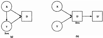
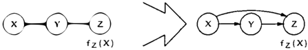
Now, the partial order--( induced by an AID I is found by initially treating I as a PID (ignoring any labels) and then refining the partial order --( 1 induced by the PID s.t. for any pair of variables X andY, where X f. 1 Y andY f.' X we have X--( Y if X E Sr (see Figure 6); if {X, Y} £; Sr we have X f. Y and Y f. X.

<•l

Figure 6: In figure (a) the AID induces the partial order X --( Y --( D, and in figure (b) the AID induces the partial order X --( Y --( D --( 0 1·

In what follows we assume that an AID has exactly one split variableS � (termed the initial split variable ) satisfying that WE Sr\{S�}: S� --( Y; Date? is the initial split variable in the AID depicted in Figure 2. Obviously, the set of variables succeeding the initial split variable s� is dependent of the state of s� hence, we define the concept of a missing variable.

Definition 5. Let I be an AID and let S� be the initial split variable in I. The chance variable X is said to be missing in I given s� = S] if:

1. fx[S� H s,] = 0 or
2. ii) 3Y E dep(X) s.t. y is missing givens � = S] or
3. iii) VS E Sr \{S�} : X --( S and X is unresolved given s� = s,.

The above definition is easily adopted to value nodes, decision nodes and informational arcs and will there­ fore not be described further.

The following definition specifies the AID obtained from another AID I by instantiating the initial split variable in I.

Definition 6. Let I = (U, £,:F) be an AID and let s� be the initial split variable in I. The AID I I = (U1, £', :F1) is said to be myopicly reduced from I given s� = s1 if:

• U' ={X E UIX is not missing givenS � = sJ}.
• £ ' {(X, Y) E £1{X, Y} C U' 1\ (X, Y) is not missing in I given s� = S] }.
• :F' = {fx[S� H s1]1fx E :F and X E U'} U {f(x,v)(S� H SJ]if(X,Yl E :F and (X, Y) E £'}.

That is, we myopicly reduce an AID I by removing the missing nodes and the missing arcs. However, the removal of arcs might render additional nodes missing thus, for all missing nodes and arcs to be removed we need to remove them iteratively. The AID I' obtained from I by iteratively removing missing nodes and arcs is said to be reduced from I given s� = S] and is denoted I[S� H s,].

Figure 3 illustrates the AID which has been reduced from the AID in Figure 2 given Date ?=n. Notice that reducing an AID w.r.t. its initial split variable S� is the same as instantiating s� hence, s� is not a split variable in I[S� H s,].

In the remainder of this paper we restrict our atten­ tion to AIDs having exactly one initial split variable. This restriction also applies to AIDs which have been reduced from other AIDs that is, we do not consider AIDs which can be reduced to an AID that does not adhere to this restriction; having a unique initial split variable ensures that the reduction is unambiguous and it does not seem to exclude any natural decision problems; actually, decision trees have the same prop­ erty. Furthermore, for ease of notation we shall treaJ restrictive variables as split variables unless stated oth erwise (Sf denotes the union of Sr and the set of H strictive variables in 1). However, we do not requir the occurrence of a unique restrictive variable as tf order in which the restrictive variables are instantiat( is of no importance, i.e., the syntactical constraint 1 the split variables does not extend to the restricti variables.

Now, based on the requirement about a unique SJ variable in an AID I we can identify the possible st

configurations in I. These configurations are found by going in the temporal order specified by I. That is, we iteratively identify the initial split variable in the AID reduced from the AID in the previous step and assign this split variable a configuration consistent with the previous one.

The initial split variable S� in I is identified as de­ scribed previously. In general the k 'th split variable in I w.r.t. the configurations= (s1,sz, ... ,sk-d, de­ noted S�k-1, is the initial split variable in I[S� H s1](S�1 H Sz]· · · (S�;_\ H Sk-1], where S�i-1 is the initial split variable in I w.r.t. the configuration Si-1 = (s1, sz, ... , S-t-1 ) . Obviously, if I ' has been re­ duced from I w.r.t. s� =51 then 51 must be a possible state for S�, i.e., each time an AID is reduced the pos­ sible outcomes/decision options for the split variables are "updated". In what follows we let I[S�i-1 H sd 1 2 . denote the AID I[SV' H s1][S5 1 H sz]· · · [S1i_1 H sd.

Definition 7. Let S{ C Sf and S{' {S1, Sz, ... , St} � S{ be subsets of the split vari­ ables contained in the AID I. A configuration s = (s1, sz, ... , st) over the variables S{' is said to be a split configuration for S{ over S{' if: =

• Si is the i'th split variable in I w.r.t. the configu­ ration S-t-1 = (s1,sz, ... ,S-t-11 and
• S is not a split variable in 1[5�1 _1 H sr], 'r/5 E S{\Sf'

If S{ = Sf then s is said to be an exhaustive split configuration for I over S{'.

For notational convenience, we will sometimes use I[S{' H s] to denote the AID reduced from the AID I w.r.t. the split configuration s over the variables S{'.

Example 2. Consider the AID depicted in Figure 2. The configuration (Date?=y) is a split configura­ tion, whereas (Date ?=y,Accept?=y, To do ?=movie) is an exhaustive split configuration. The configuration (Date?=n,Club?=n) is an exhaustive split configura­ tion also since Date?=n implies that Accept? is never observed, thereby rendering the variables Movie, Menu and To Do? missing. D

Based on the notion of a split configuration we can de­ termine the contexts in which a decision variable can occur. A context for a decision variable 0 is a config­ uration s = ( w, x), where:

• s is a split configuration for S{ over the variables S{' satisfying that there does not exist a split vari­ able S E Sr[S ! 'Hs] s.t. S -< 0 in I [S{' H s].
• x is a configuration over the restrictive variables for 0 in I [S{' H s].

The set of contexts in which a decision variable 0 can occur is denoted Oo.

4 SOLVING ASYMMETRIC INFLUENCE DIAGRAMS

Solving an AID is the same as determining an optimal strategy for the decisions involved. However, as op­ posed to the PID we can not restrict our attention to the variables being required for the decision variable in question; the variables being required for 0 may vary depending on the context in which 0 appears. Thus we define a strategy as follows:

Definition 8. A strategy for an AID I is a set of func­ tions .1 ={&olD E Uo}, where bo is a decision func­ tion given by:

where pred(D ls is the set of variables preceding 0 un­ der the partial order induced by the AID which has been reduced from I w.r.t. s.

A strategy that maximizes the expected utility is termed an optimal strategy, and a decision function 60 that maximizes the expected utility for decision 0 w.r.t. each context s E Oo is termed an optimal strategy for 0.

A well-defined AID (specified in the following section) can in principle be solved by unfolding it into a de­ cision tree, and then use the "average-out and fold­ back" algorithm on that tree; the partial probability potentials specified by the realization of the AID can be seen as a model of the uncertainty associated with the chance variables (this is somewhat similar to the approach found in [Call and Miller, 1990]). However, this "brute force" approach would create an unneces­ sary large decision tree in case the original decision problem specifies symmetric subproblems.

4.1 DECOMPOSING ASYMMETRIC INFLUENCE DIAGRAMS

In this section we present an algorithm for solving AIDs. The main idea underlying the algorithm is to decompose the decision problem into a collection of symmetric subproblems organized in a tree struc­ ture, and then propagate from the leaves towards the root using existing evaluation methods to solve the "smaller" symmetric subproblems.

The decomposition is performed by reducing the AID w.r.t. the possible states of its initial split variable. This reduction is then applied iteratively to the AIDs produced in the previous step until no split variables remain. For instance, Date? is the initial split variable

in "the dating problem" depicted in Figure 2 so by decomposing the problem w.r.t. Date?=no we obtain the AID depicted in Figure 3, where the initial split variable is Night Club?. An optimal strategy can then be found by iteratively eliminating the so-called free variables in each of the subproblems:

Definition 9. Let I[S� H s,] be the AID reduced from the AID I. The variable X is said to be free in I[S� H s,] if S� -< X and VS E Sr[S � �-+ s !l : X -< S, where-< is the partial order induced by I[S� H s,]. If X is not free in I[S� H s,] then X is said to be bound in I[S� H s1].

The evaluation of an AID I is initiated by invoking the algorithm Evaluation on I; note that in the follow­ ing algorithms we exploit that instantiating the initial split variable in an AID produces another AID with a unique initial split variable.

Algorithm 1 (Evaluation). Let I be an AID and let S� be the initial split variable in I. If Evaluation is invoked on I, then

1. Invoke Evaluation on I[S� H s,], Vs1 E W5 1 · v
2. ii) Absorb the potentials from I[S� H s,] to I, Vs1 E W51 . v
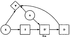
3. iii) Let 11> be a utility potential absorbed (Algorithm 2} from I[S� H s�] s.t. S� rf. dom(1!>). If :Jj -# i s. t 11> is not absorbed from I [S� H S�] to I then condition 11> on S = s� (see Figure 7).

Algorithm 2 (Absorption). Let I[S1t_ 1 H Si] be an AID and let S be the initial split variable in I[S1i-1 H sil· If Absorption is invoked on I [S1 i _ 1 H Si][S H s] from I[S1t_1 H si], then:

1. Let X be the free variables I[S1i_1 H Si][S H s] and set 1\ = {i\ E <D rrs�i-1 �-+sd[ S�-+ s l U 'l' r rs�i - 1 �-+s t H S�-+sli:J X EX s.t. X E dom(i\)}.
2. ii) Eliminate the variables X from 1\ w.r.t. the par­ tial order induced by I[St_ 1 H si][S H s] {Al­ gorithm 3}. Let <I>i[ So-+s] and '1'irs�-+ s l be the sets
3. of probability potentials and utility potentials ob­ tained.
4. iii) For each i\ E /\, remove i\ from I[S�. J associate <Dj[ S �-+ s] U'l'j[ So-+s ] with I[S�; alll � j � i. 1 H Sj] and 1 Hsj],for

The algorithm below describes the elimination of variables, and is inspired by the lazy evaluation architecture [ Madsen and Jensen, 1999 ] . However, any elimination algorithm can in principle be used.

Algorithm 3 (Elimination). Let I be an AID and let <D I and '¥I be the sets of probability and utility po­ tentials associated with I. If Elimination of variable X is invoked on <D I U 'l'I, then:

1. Set <Dx = {cl:> E <l>IIX E dom(cl:>)} and 'l'x = {1!> E 'l'IIX E dom(1!>)}.
2. ii) Calculate:

where M is a marginalization operator depending on the type of X, i.e., M denotes a summation if X is a chance variable and a maximization if X is a decision variable.

During the evaluation, the decision option maximizing the utility potential from which a decision variable 0 is eliminated should be recorded as the optimal strategy for 0 w.r.t. to the context in question.

Now, based on the algorithms above we define the con­ cept of a well-defined AID. The definition is based on the notion of a significant chance variable, which can be adopted from the PID framework by consider­ ing the admissible total orderings of the free variables in each of the AIDs produced during the decompo­ sition; the structural characterization of the chance variables being significant for a given decision variable ( see [ Nielsen and Jensen, 1999b ] ) can also be adopted to an AID I, except that we have to investigate each of the AIDs reduced from I w.r.t. the exhaustive split configurations for I.

Definition 10 (Well-defined). An AID I is said to define a decision scenario if:

• for all split configurations s, there does not exist a free chance variable A and a free decision variable

• 0 in I [S{' H s] s.t. A is significant for 0; s is a configuration over the variables S{' � Sf
• for any decision variable 0 and for each context s = ( w, x) for 0 there does not exist two restric­ tive functions Yb and Yb s.t. dom(y b ) � n�ls and dom(y b ) � n�ls' where n�ls is the set of restrictive variables which are present in I given s.

Theorem 2 (Sound). If Algorithm 1 is invoked on an AID I which define a decision scenario, then Algo­ rithm 1 computes an optimal strategy for each decision variable in I .

Proof. The idea of the proof is to initially treat non­ split variables as split variables, thereby obtaining a decision tree representation of the decision problem when reducing the AID; each subproblem contains ex­ actly one free variable which corresponds to a node in the decision tree. Note that from Algorithm 1 we have that treating non-split variables as split variables has no impact on the evaluation.

Finally, we exploit that the set of partial probability potentials constitutes a model of the uncertainty as­ sociated with the chance variables, and from this it can be shown that the calculations performed by Al­ gorithm 1 are equivalent to the calculations peformed when solving the corresponding decision tree. For fur­ ther detail see [Nielsen and Jensen, 1999a]. D

5 CONCLUSION

In this paper we have presented a framework, termed asymmetric influence diagrams, for representing asym­ metric decision problems. The asymmetric influence diagram is based on the partial influence diagram and uses labels, associated with nodes and informational arcs, to encode structural asymmetry at the qualita­ tive level. Asymmetry which deals with the possible outcomes of an observation or the legitimate decision options of a decision variable is represented in partial probability potentials and restrictive functions, respec­ tively.

We have presented an algorithm for solving asymmet­ ric influence diagrams. The algorithm decomposes the asymmetric decision problem into a collection of sym­ metric subproblems which can be solved using existing methods for solving influence diagrams.

As part of the future work, the class of asymmetric de­ cision problems which can be modeled effectively using AIDs needs to be determined. We claim that the lan­ guage of AIDs is as strong as that of decision trees, but the amount of redundancy in the models should be determined.

References

• [Bielza and Shenoy, 1999] Bielza, C. and Shenoy, P. P. ( 1999). A Comparison of Graphical Techniques for Asymmetric Decision Problems. Management Sci­ ence, 45(11):1552�1569.

[Call and Miller, 1990] Call, H. J. and Miller, W. A. (1990). A comparison of approaches and implemen­ tations for automating decision analysis. Reliability Engineering and System Safety, 30: 115� 162.

[Covaliu and Oliver, 1995] Covaliu, Z. and Oliver, R. M. (1995). Representation and Solution of Deci­ sion Problems Using Sequential Decision Diagrams. Management Science, 41(12):1860�1881.

[Madsen and Jensen, 1999] Madsen, A. L. and Jensen, F. V. (1999). Lazy evaluation of symmetric bayesian decision problems. In Proceedings of the Fifthteenth Conference on Uncertainty in Artificial Intelligence. Morgan Kaufmann Publishers.

• [Nielsen and Jensen, 1999a] Nielsen, T. D. and Jensen, F. V. (1999a). Representing and solving asymmetric bayesian decision problems. Technical report, Department of Computer Science, Fredrik Bajers 7C, 9220 Aalborg, Denmark. R-99-5010.
• [Nielsen and Jensen, 1999b] Nielsen, T. D. and Jensen, F. V. (1999b). Welldefined decision scenar­ ios. In Proceedings of the Fifthteenth Conference on Uncertainty in Artificial Intelligence. Morgan Kaufmann Publishers.
• [Qi et al., 1994] Qi, R., Zhang, N. 1., and Poole, D. ( 1994). Solving asymmetric decision problems with influence diagrams. In Proceedings of the Tenth Conference on Uncertainty in Artificial Intelligence, pages 491�497. Morgan Kaufmann Publishers.
• [Shenoy, 1992] Shenoy, P. P. (1992). Valuation-based Systems for Bayesian Decision analysis. Operations Research, 40(3) :463�484.
• [Shenoy, 2000] Shenoy, P. P. (2000). Valuation net­ work representation and solution of asymmetric de­ cision problems. European Journal of Operations Research, 121 (3) :579�608.
• [Smith et al., 1993] Smith, J. E., Holtzman, S., and Matheson, J. E. (March/ April 1993). Structuring conditional relationships in influence diagrams. Op­ erations research, 41 (2) :280�297.
• [Tatman and Shachter, 1990] Tatman, J. A. and Shachter, R. D. (March/ April 1990). Dynamic Pro­ gramming and Influence Diagrams. IEEE Transac­ tions on Systems, Man and Cybernetics, 20(2):365� 379.