Sampling First Order Logical Particles

Hannaneh Hajishirzi and Eyal Amir

Department of Computer Science University of Illinois at Urbana-Champaign { hajishir, eyal } @uiuc.edu

Abstract

Approximate inference in dynamic systems is the problem of estimating the state of the system given a sequence of actions and partial observations. High precision estimation is fundamental in many applications like diagnosis, natural language processing, tracking, planning, and robotics. In this paper we present an algorithm that samples possible deterministic executions of a probabilistic sequence. The algorithm takes advantage of a compact representation (using first order logic) for actions and world states to improve the precision of its estimation. Theoretical and empirical results show that the algorithm's expected error is smaller than propositional sampling and Sequential Monte Carlo (SMC) sampling techniques.

1 Introduction

Important AI applications like natural language processing, program verification, tracking, and robotics involve stochastic dynamic systems. The current state of such systems is changed by executing actions. Reasoning is the task of computing the posterior probability over the state of such dynamic systems given past actions and observations. Reasoning is difficult because the system's exact initial state or the effects of its actions are uncertain (e.g., there may be some noise in the system or its actions may fail).

Exact reasoning (e.g., [11; 1]) is not tractable for long sequence of actions in complex systems. This is because domain features become correlated after some steps, even if the domain has much conditional-independence structure [4]. Therefore, approximate reasoning is of much interest. One of the most commonly used classes of techniques for approximate reasoning is SMC sampling [5]. These methods are efficient, but they require many samples (exponential in the dimensionality of the domain) to yield a lower error rate. Recently, [8] introduced a new sampling approach which achieves higher precision than SMC techniques given a fixed number of samples. Still, it requires a large number of samples in complex domains because in their method the domains are represented using propositional logic.

In this paper we present a sampling-based filtering algorithm in a first order dynamic system called Probabilistic Relational Action Model (PRAM) . We show that our new algorithm takes fewer samples and yields better accuracy than previous sampling techniques. Such improvement is possible because of the underlying deterministic structure of the transition system, the compact representation of the domains using first order logic (FOL), and efficient subroutines for first order logical regression (e.g., [17]) and first order logical filtering [19; 14].

Wemodel a PRAM (Section 2) using probabilistic situation calculus [17], extended with a first order probabilistic prior that combines FOL and probabilities in a single framework (e.g., [18; 3; 12; 15; 7; 20]). Transitions in a PRAM are modeled with probability distributions over possible deterministic executions of probabilistic actions (every transition model can be represented this way).

Our algorithm (Section 3) first samples sequences of deterministic actions, called first order (FO) particles , that are possible executions of the given probabilistic action sequence and are consistent with the observations. It also updates the current state of the system given each FO particle. Next, the algorithm computes the probability of the query given the updated current state. To do so, it applies logical regression to the query for each FO particle, computes a FOL formula that represents all the possible initial states, and computes the prior probability of that formula. Finally, the algorithm computes the posterior probability as the weighted sum of these derived prior probabilities.

This algorithm achieves superior precision with fewer samples than SMC sampling techniques [5]. The intuition behind this improvement is that each FO particle corresponds to exponentially many state sequences (particles) generated by earlier techniques. The algorithm is computationally efficient when FOL regression and filtering with the deterministic actions are efficient. We prove our claim about precision and verify the results empirically by several experiments (Section 4).

Our representation for PRAM differs from Dynamic Bayesian Networks (DBNs) (e.g., [13]). DBNs emphasize conditional independence among random variables. In contrast, our model applies a representation for the transition model as a distribution over deterministic actions. Also, PRAM uses a different model for observations. The observations are received asynchronously without prediction of what will be observed. Both frameworks are universal and can represent each other, but they are more compact and natural in different scenarios.

The closest work to ours is [8] which also samples deterministic executions of the given probabilistic sequence. However, that work assumes that the deterministic sequences are always executable. In this paper we relax this assumption and avoid sampling the sequences that are not executable by keeping track of the current state of the system. Also, our representation is more compact (uses FOL), so it achieves higher precision with less samples.

Recently, [10; 22] explore reasoning algorithms in relational HMMs. They use a different representation than ours for their observations. Moreover, they do not use a compact representation for their prior distribution. Earlier algorithm trades efficiency of computation for precision as it is an exact method. Latter, introduced a sampling algorithm where each sample represents a set of states and is generated from the probability distribution over disjoint sets of the states. Therefore, to update this distribution they build new disjoint sets at each time step which leads to a large number of disjoint sets (exponential in domain features) in long sequences. Our algorithm is different in a sense that we do not sample states; we sample deterministic sequences which correspond to state sequences that are derived by regressing the query through the deterministic sequence.

2 Probabilistic Relational Action Models

In this section we present our framework, called Probabilistic Relational Action Model (PRAM), for representing the dynamic system. The system is dynamic in a sense that its state changes by executing actions. Actions have probabilistic effects that are represented with a probability distribution over possible deterministic executions.

A PRAM consists of two main parts: (1) A prior knowledge representing a probability distribution P 0 over initial world states in a relational model. (2) A probability distribution PA over deterministic executions of probabilistic actions. In what follows we define the basic building blocks of a PRAM. We first define the language L of a PRAM for representing the probability distributions:

Definition 1. [PRAM language] The language L of a PRAM is a tuple ( F, C, V, A , D A ) consisting of:

• F a finite set of predicate variables (called fluents ) whose values change over time.
• C a finite set of constants representing objects in the domain.
• V a finite set of variables.
• A , D A finite sets of probabilistic and deterministic action names, respectively.

We define a fluent atom as a formula of the form f ( x 1 , . . . , x k ) (also represented by f ( glyph[vector] x ) ), where x 1 , . . . , x k ∈ V ∪ C are either variables or constants. In PRAM grounding of a fluent f ( glyph[vector] x ) is defined as replacing each variable in glyph[vector] x with a constant c ∈ C . Accordingly, a world state s ∈ S is defined as a full assignment of { true , false } to all the groundings of all the fluents in F .

Example 1 (Briefcase) . Briefcase is a domain consisting of objects , locations , and a briefcase B . The variables ? o and ? l denote objects and locations , respectively. The fluents are: In (? o ) , At ( B, ? l ) , At (? o , ? l ) . An agent interacts with the system by executing some probabilistic actions: putting objects in, PutIn (? o, B ) , taking objects out of the briefcase, TakeOut (? o, B ) , and moving the briefcase with objects inside, Move ( B, ? l 1 , ? l 2 ) . Some deterministic actions in the domain are: MvWithObj , PutInSucc , and PutInFail .

In PRAM each deterministic action da ( glyph[vector] x ) ∈ D A is specified by precondition and successor state axioms [17].

Definition 2. [Deterministic action axioms] Precondition axioms show the conditions under which the deterministic action da is executable in a given state; Precond is a special predicate denoting the executability of a deterministic action: Precond da ( glyph[vector] x ) ⇔ Φ( glyph[vector] x ) where Φ is a FOL formula.

Successor state axioms enumerate all the ways that the value of a particular fluent can be changed; A successor state axiom for a fluent f is defined as:

where Succ t f,da ( glyph[vector] x ) is a FOL formula at time t . One can easily derive the effects of actions by the above axioms.

For example, the precondition of the deterministic action MvWithObj ( B, ? l 1 , ? l 2 ) is At ( B, ? l 1 ) ∧ ¬ At ( B, ? l 2 ) , and its effect is ¬ At ( B, ? l 1 ) ∧ At ( B, ? l 2 ) ∧ ( ∀ ? o In (? o ) ⇒ At (? o, ? l 2 )) .

The grounding of a deterministic action is defined as the grounding of all the fluent atoms appearing in the precondition and effect logical formulas Precond t da ( glyph[vector] x ) and Succ t f,da ( glyph[vector] x ) . Therefore, a grounded deterministic action is a transition function T : S × D A → S . One can see from the example that for grounding the action MvWithObj , one needs to permute all the possible combinations of objects inside the briefcase . This increases the dimensionality of the domain and increases the required number of samples to yield low error. Hereinafter for simplicity, we represent fluents and actions without their arguments whenever it is not necessary to mention the variables or domain objects.

Definition 3. [Probability distribution for probabilistic actions] Let ψ 1 . . . ψ k be FOL formulas (called partitions ) that divide the world states into mutually disjoint sets. Then, PA ( da | a, s ) is defined as a probability distribution over possible deterministic executions da of the probabilistic action a in the state s which satisfies one of the partitions ψ i ( i ≤ k ) . More formally, when some state s satisfies partition ψ i then PA ( da | a, s ) = PA i ( da ) , where PA i is a probability distribution over different deterministic executions da of action a corresponding to the partition ψ i .

We assume that replacing variables in a ( glyph[vector] x ) with constants does not change PA ( da ( glyph[vector] x ) | a ( glyph[vector] x ) , s ) .

For example, for probabilistic action TakeOut (? o ) , deterministic action TakeOutSucc (? o ) , and s | = ψ 1 = In (? o ) : PA ( da | a, s ) = PA 1 ( TakeOutSucc (? o )) = 0 . 9 .

In PRAM we assume a prior distribution over world states at time 0 . Models like [18] are used to represent probabilities in relational models. A knowledge engineer can define the semantics of the prior distribution by using each of these models. Then, we use the inference algorithm defined in that model's semantics to compute probability of formulas at time 0 . Our filtering algorithm does not depend on the way the initial knowledge has been represented. We discuss more about this in Section 3.1.3.

In conclusion, we define a PRAM formally as follows: Definition 4. A PRAM is a tuple ( L , AX , PA , P 0 ) as:

• Language L = ( F, C, V, A , D A ) representing the language of PRAM (Definition 1)
• Aset of deterministic action axioms AX (Definition 2)
• Aprobability distribution PA for each probabilistic action (Definition 3)
• A prior distribution P 0 over initial world states

Based on the aforementioned dynamic system, PRAM, we define our stochastic filtering problem as computing probability of a query given a sequence of probabilistic actions and observations. The query is defined as a FOL formula ϕ T at the final time step, T . Note that throughout the paper superscripts represent time. Each a t in the probabilistic action sequence 〈 a 1 , . . . , a T 〉 represents the probabilistic action that has been executed at time t .

The observations 〈 o 0 , . . . , o T 〉 are given asynchronously in time without prediction of what we will observe (thus,

this is different from HMMs [16], where a sensor model is given). Each observation o t is represented with a FOL formula over fluents. When o t is observed at time t , the FOL formula o t is true about the state of the world at time t . We assume that a deterministic execution da of the probabilistic action a t in the sequence does not depend on the future observations.

3 Filtering Algorithm

In this section we present our filtering algorithm for computing probability of a query ϕ T given a sequence of probabilistic actions a 1: T = 〈 a 1 , . . . , a T 〉 and observations o 0: T = 〈 o 0 , . . . , o T 〉 in a PRAM. The algorithm approximates this probability by generating samples among possible deterministic executions of the given probabilistic action sequence. Then, it places those samples instead of the enumeration of deterministic executions and marginalizes over those samples. The following equation shows the exact computation.

where glyph[vector] DA i is a possible execution of the sequence a 1: T .

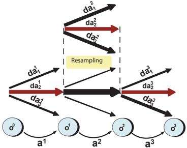
The first step of our approximate algorithm is generating N samples (called FO particles ) from all the possible deterministic executions of the given probabilistic sequence. Two different sampling algorithms are introduced in Section 3.2. The algorithms (illustrated in Figure 1) generate a weighted FO particle glyph[vector] DA i with weight w i given the sequence a 1: T and the observations o 0: T from the probability distribution P ( glyph[vector] DA i | a 1: T , o 0: T ) .

The next step of the algorithm is computing P ( ϕ T | glyph[vector] DA i , o 0: T ) for each FO particle glyph[vector] DA i . It does

PROCEDURE FOFA ( SampleAlg , ϕ T , a 1: T , o 0: T )

Input : Sampling algorithm SampleAlg , probabilistic sequence a 1: T , observations o 0: T , and query ϕ T

Output :

˜ P ( ϕ T | a 1: T , o 0: T )

1. ( glyph[vector] DA 1: N , curF 1: N ) ← SampleAlg ( a 1: T , o 0: T )

1. for each glyph[vector] DA i compute PFOF ( ϕ T , glyph[vector] DA i , curF i )

1. return ˜ P ( ϕ T | a 1: T , o 0: T ) using Equation (6).

Figure 2: FOFA: First Order Filtering Algorithm for approximating P ( ϕ t | a 1: t , o 0: t ) given a sampling algorithm SampleAlg (either S/R-Actions (Figure 5) or S-Actions (Figure 6)). Italic fonts is used to denote subroutines.

so (Section 3.1) by updating the current state of the system and then computing the posterior probability conditioning on the updated current state.

Finally, the algorithm uses generated samples in place of glyph[vector] DA i in Equation (2) and computes ˜ P N ( ϕ T | a 1: T , o 0: T ) as an approximation for the posterior probability of the query ϕ T given the sequence a 1: T and the observations o 0: T by using the Monte Carlo integration [5]:

Details of each step of our first order filtering algorithm ( FOFA , Figure 2) are explained next. We first present the step of computing P ( ϕ T | glyph[vector] DA i , o 0: T ) because it is used as a subroutine in the sampling algorithms.

3.1 Probability of a FOL Formula at time t

In this section we show how to compute the probability P ( ϕ t | glyph[vector] DA , o 0: t ) of the formula ϕ t given a FO particle glyph[vector] DA and observations o 0: t . Executing the FO particle glyph[vector] DA with observations o 0: t updates the current state of the system. The current state is derived by applying a FO progression subroutine (described below) at each time step. Afterwards, procedure PFOF (Figure 3) computes the probability of the query given the current state of the system for each FO particle. Its first step applies a FO regression subroutine to the query and the current state formula and as output returns FOL formulas at time 0. This can be done since the actions are deterministic. The algorithm's second step computes the prior probability of the regression of the query conditioned on the current state formula regressed by the FO particle; Recall that a FO particle is a sampled sequence of deterministic actions.

3.1.1 Progress Current State Formula

We define the current state formula as a FOL formula representing the set of states that are true after executing a sequence of deterministic actions and receiving observations. In this section we present algorithm Progress that updates the current state formula given a deterministic action and an observation. In general, progressing a FOL for-

PROCEDURE

PFOF ( ϕ t , glyph[vector] DA , curF )

Input : FO particle glyph[vector] DA and the current state formula curF Output : P ( ϕ t | glyph[vector] DA , o 0: t )

1. ϕ 0 ← RegSeq ( ϕ t , glyph[vector] DA )
2. curF 0 ← RegSeq ( curF , glyph[vector] DA )
3. p 0 ← Prior-FOF ( ϕ 0 | curF 0 )
4. return P ( ϕ t | glyph[vector] DA , o 0: t ) ← p 0

PROCEDURE Prior-FOF ( ϕ 0 , M

Input : Formula ϕ 0 , Markov network M MLN of the prior MLN Output : P ( ϕ 0 )

MLN )

1. ∧ i C i ← ConvertToCNF( ϕ 0 )
2. Define indicator functions as Equation (4)
3. M ← ConstructNetwork ( M MLN , fluents of ϕ 0 )
4. return P ( ϕ 0 ) by performing inference on M

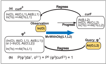
Figure 4: (a) Regressing query ϕ 1 and curF by MvWithObj . Note, L 1 , L 2 , and O are constants, and there are only two possible locations L 1 and L 2 , i.e. At ( O,L 2) ≡ ¬ At ( O,L 1) . (b) Computing P ( ϕ 2 | glyph[vector] DA,o 0:1 ) using Lemma 1.

mula δ with a deterministic action da , Progress ( δ, da ) , results in a set of FOL formulas ∆( p 1: n ) where p 1 , . . . , p n are atomic subformulas of ∆ and δ ∧ Precond da | = ∆( Succ p 1 ,da , . . . , Succ p n ,da ) (see [19] for more details). Also, filtering a FOL formula δ with an observation o is the FOL formula δ ∧ o .

Overall, generating all ∆ s is impossible because there are infinitely many such ∆ s. In this paper we assume that progression of the current state formula curF with a deterministic action da , Progress ( curF , da, o ) , is representable with a FOL formula. Hence, it is equal to ∨ i ∆ i ( p 1: n ) ∧ o . Furthermore, [19; 14] provide some special conditions that the progression algorithm is polynomial and the representation of progressing a formula is compact. For example, progressing In ( O ) through deterministic action MvWithObj ( L 1 , L 2) results in the formula At ( B,L 2) ∧ In ( O ) ∧ At ( O,L 2) ∧ ( ∀ ? o In (? o ) ⇒ At (? o, L 2)) .

3.1.2 Regressing a FOL Formula

Procedure RegSeq takes a FOL formula ϕ t and a FO particle glyph[vector] DA and returns as output another FOL formula ϕ 0 . ϕ 0 represents the set of possible initial states, given that the fi- nal state satisfies ϕ t , and the FO particle glyph[vector] DA occurs. Thus, every state that satisfies ϕ 0 leads to a state satisfying ϕ t after glyph[vector] DA occurs.

For a deterministic action da t and a FOL formula ϕ t , the regression Regress ( ϕ t , da t ) of ϕ t through da t is a FO formula ϕ t -1 such that state s t -1 satisfies ϕ t -1 iff the result of the transition function T ( s t -1 , da t ) satisfies ϕ t . The computation of the regression RegSeq ( ϕ t , glyph[vector] DA ) of ϕ t through the FO particle glyph[vector] DA is done recursively.

Regression of the current state formula curF is defined similar to the regression of formula ϕ t since the current state is also represented with a fist order formula.

The algorithm for regression Regress ( ϕ t , da ) of formula ϕ t with deterministic action da works as follows (see [17]). Suppose that ϕ t is an atomic fluent f t ( glyph[vector] x ) with the successor state axiom Succ t -1 f,da ( glyph[vector] x ) . Then, we derive the regression of ϕ t by replacing f t ( glyph[vector] x ) with Succ t -1 f,da ( glyph[vector] x ) . The regression of non-atomic formulas are derived inductively as follows:

• Regress ( ¬ ϕ t ) = ¬ Regress ( ϕ t )
• Regress ( ϕ t 1 ∧ ϕ t 2 ) = Regress ( ϕ t ) ∧ Regress ( ϕ t 2 )
• Regress (( ∃ ν ) ϕ t ) = ∃ ν Regress ( ϕ t )

The efficiency of the regression yields from the fact that we regress non-grounded fluents f ( glyph[vector] x ) . Besides, one can employ some approximations at each step (like removing unnecessary clauses) to maintain the compactness of the regressed formulas.

We now summarize and show how to compute the probability distribution P ( ϕ t | glyph[vector] DA , o 0: t ) by applying progression and regression. The algorithm first computes curF by progressing through the FO particle and observations. Then, it computes ϕ 0 and curF 0 by regressing ϕ t and curF . Finally, it computes P 0 ( ϕ 0 | curF 0 ) as the evaluation of P ( ϕ t | glyph[vector] DA, curF ) as shown by the following lemma.

Lemma 1. Let ϕ t be the query and o 0: t the observations. If curF is the current state formula, ϕ 0 = RegSeq ( ϕ t , glyph[vector] DA ) , and curF 0 = RegSeq ( curF , glyph[vector] DA ) , then P ( ϕ t | glyph[vector] DA , o 0: t ) = P 0 ( ϕ 0 | curF 0 ) .

Proof. Probability of a formula is a marginalization over states: P ( ϕ t , o 0: t | glyph[vector] DA ) = ∑ s P ( ϕ t , curF | s, glyph[vector] DA ) P ( s | glyph[vector] DA ) . For s , P ( ϕ t , curF | s, glyph[vector] DA ) = 1 if s | = ϕ 0 ∧ curF 0 , o.w. it is 0 . The reason is that executing the deterministic sequence glyph[vector] DA in state s results at time t that models ϕ t and is consistent with observations o 0: t iff s | = ϕ 0 ∧ curF 0 . Therefore, P ( ϕ t , o 0: t | glyph[vector] DA ) = ∑ s | = ϕ 0 , curF 0 P ( s ) = P 0 ( ϕ 0 , curF 0 ) .

The same computations exist for P ( o 0: t | glyph[vector] DA ) . Therefore,

Figure 4 shows an example of computing P ( ϕ t | glyph[vector] DA,o 0: t ) using procedure PFOF . The next section shows how to compute P 0 ( ϕ 0 | curF 0 ) using the prior P 0 . Note that ϕ 0 and curF 0 are FOL formulas over fluents at time 0 .

3.1.3 Prior Probability of a FOL Formula

In this section we describe procedure Prior-FOF to compute the probability of a FOL formula at time 0. We assume that the prior distribution P 0 over world states of a PRAM with language L = ( F, C, V, A , D A ) is represented by a Markov Logic Network (MLN) [18]. We choose to represent our prior probabilistic logic with an MLN (called prior MLN ) because it keeps the expressive power of FOL for a fixed domain.

Our prior MLN consists of a set of weighted FOL formulas over the fluents in language L of the PRAM. The semantics of the MLN is that of a Markov network M MLN [9] whose cliques correspond to groundings of the formulas given the universe of objects C ∈ L . The potential Φ of a clique Cl is defined as the exponential of the weight of the corresponding formula in case the grounding is true.

We introduce Prior-FOF (Figure 3) to compute the probability of a FOL formula ϕ 0 by slightly changing the inference algorithm expressed for MLNs. Procedure Prior-FOF first converts ϕ 0 to a clausal form; Note that like MLNs existentially quantified formulas are replaced by disjunction of their groundings. Then, Prior-FOF assigns an indicator function, I g ( C i ) , to every grounding g of a clause C i .

The next step is to construct a Markov network M as the minimal subset of the original network M MLN required to compute P 0 ( ϕ 0 ) . The nodes in M consist of all the ground fluents f g ( C i ) in clauses C i of ϕ 0 and all the nodes in the original Markov network M MLN with a path to the fluent f g ( C i ) . The final step is to perform inference on this network. It can be computed exactly by performing variable elimination (e.g., [9]) in P 0 ( ϕ 0 ) ∝ ∑ f ∈ M ∏ glyph[vector] f j ∈ Cl j , glyph[vector] f i ∈ C i Φ j ( glyph[vector] f j ) I ( glyph[vector] f i ) . Also, one can employ any approximate inference algorithm like Gibbs sampling.

We are not restricted to use MLNs as a framework for representing prior probability distribution. We can use any other probabilistic logical frameworks ([3; 12; 15; 7; 20]) provided that the expressed inference algorithm in that framework can compute probability of the query. Note that the query ϕ 0 for that framework is derived from the regression of the original query ϕ t given an FO particle. Also, our algorithms would work for unbounded domains just by using a framework (e.g., [21]) for representing prior distribution over infinite states.

PROCEDURE S/R-Actions ( a 1: T , o 0: T ) Input : Probabilistic sequence a 1: T and observations o 0: T Output : N FO particles glyph[vector] DA 1: N 1. for n ← 1 . . . N : curF n ← o 0 2. for t ← 1 . . . T 3. for n ← 1 . . . N 4. π ← ∑ ψ i PA i · PFOF ( ψ t -1 i , da 1: t -1 ) 5. P ← ∑ ψ i PA i · PFOF ( ψ t -1 i , da 1: t -1 n , curF n ) 6. ˆ da t ← a sample from probability distribution π 7. curF n ← Progress ( curF n , ˆ da t n , o t ) 8. w ∗ n ← π ( ˆ da t n ) P ( ˆ da t n ) 9. 〈 ˆ w 1 , . . . , ˆ w N 〉 ← Normalize ( w ∗ 1 , . . . , w ∗ N ) 10. ( da t 1: N , w 1: N ) ← Resample ( ˆ da t 1: N , ˆ w 1: N ) 11. return glyph[vector] DA 1: N ←〈 da 1 . . . da T 〉 1: N

PROCEDURE S-Actions ( a 1: T , o 0: T ) Input : Probabilistic sequence a 1: T and observations o 0: T Output : N FO particles glyph[vector] DA 1: N 1. for n ← 1 . . . N : curF n ← o 0 2. for t ← 1 . . . T 3. for n ← 1 . . . N 4. P ← ∑ ψ i PA i · PFOF ( ψ t -1 i , da 1: t -1 , curF n ) 5. da t ← a sample from probability distribution P 6. curF n ← Progress ( curF n , da t , o t ) 7. return glyph[vector] DA 1: N ←〈 da 1 . . . da T 〉 1: N

3.2 Sampling Algorithms

In this section we describe procedures S/R-Actions (Figure 5) and S-Actions (Figure 6) which generate N samples (called FO particles ) given a sequence of probabilistic actions and observations. Each FO particle is a possible deterministic execution of the given probabilistic sequence. Both algorithms incrementally build every FO particle by sampling a deterministic action at a time. Later, we will discuss about the deficiencies of S/R-Actions algorithm.

Both S/R-Actions and S/Actions generate a FO particle glyph[vector] DA = 〈 da 1 , . . . , da T 〉 given a sequence a 1: T and observations o 0: T from the distribution P ( glyph[vector] DA | a 1: T , o 0: T ) . We compute this probability distribution iteratively:

The above derivation allows iterative sampling of deterministic actions from the distribution P ( da t | a t , da 1: t -1 , o 0: t ) . Recall that a FO particle is a sequence of deterministic actions. Thus, at each time the algorithms sample a deterministic action da t given the probabilistic action a t , the previous deterministic actions da 1: t -1 , and the previous obser- vations o 0: t ; Note that current deterministic action is independent of the future observations. Then, the algorithms update the current state formula curF (Section 3.1.1) given the current deterministic action and the observation.

Algorithms S/R-Actions , S-Actions use different approaches for incremental sampling of each deterministic action. In S/R-Actions , we adopt a sequential importance sampling approach. At each time step, S/R-Actions samples deterministic actions based on a normalized importance function, assigns weights to the particles, and resamples if the weights have high variance. The importance function π ( da t | a t , da 1: t -1 ) approximates P ( da t | a t , da 1: t -1 , o 0: t ) by ignoring the effect of the current state curF in the PRAM = ( L , AX , PA , P 0 ) .

where ψ i,a t is the i th partition of action a t (Definition 3).

At time step t , S/R-Actions samples N deterministic actions da t 1: N from the importance function: π ( da t | a t , da 1: t -1 ) . It then restructures the n th particle glyph[vector] DA t -1 n by attaching the deterministic action da t n to that particle, i.e. glyph[vector] DA t n = 〈 da 1 n , . . . , da t -1 n , da t n 〉 . The importance weight w ∗ n of the n th particle is derived as: w ∗ n = P ( da t n | a t ,da 1: t -1 n ,o 0: t ) π ( da t n | a t ,da 1: t -1 n ) .

Accordingly, the normalized importance weight w n of the n th particle is: w n = w ∗ n ∑ N i =1 w ∗ i .

The exact value for P ( da t | a t , da 1: t -1 , o 0: t ) is computed using PFOF subroutine (Figure 3).

S/R-Actions resamples the particles if the variance of the normalized importance weights becomes too high. The basic idea of resampling is to avoid those particles with very low weight and concentrate on particles that have higher normalized weight. An estimation (see [5]) for measuring high variance among the weights is estimating the effective number of particles as ̂ N eff = 1 ∑ N i =1 w i . If ̂ N eff is smaller than a threshold then procedure Resample generates a new deterministic action da t from the probability distribution over the normalized weights w 1: N of the particles. It then assigns equal weights, 1 N , to all the particles.

The second sampling algorithm, S-Actions (Figure 6), is derived by simplifying the above sampling algorithm. This algorithm at each time step generates samples among executable deterministic actions. It samples every deterministic action in a FO particle from the exact computation for P ( da t | a t , da 1: t -1 , o 0: t -1 ) (Equation 5) instead of sampling from the importance function and assigning weights. Therefore, all the weights are equal to 1 N .

S/R-Actions , samples deterministic actions even when they are not executable and assigns weight zero to those particles. Therefore, it decreases the effective number of samples. Resampling step does not help that much because it resamples the latest deterministic action in the FO particle. However, resampling earlier deterministic actions may result in a more effective set of FO particles. Note that this new type of resampling is not tractable. Therefore, it makes more sense to maintain the current state formula curF as in S-Actions and just sample executable deterministic actions (as in S-Actions ) unless there exists a better resampling procedure. In the empirical results we examine the effects of using S/R-Actions and S-Actions sampling algorithms in the FOFA filtering algorithm (Figure 2).

3.3 Correctness, Complexity, and Accuracy

The following theorem shows how FOFA with S-Actions and S/R-Actions compute the approximate posterior distribution ˜ P N ( ϕ T | a 1: T , o 0: T ) .

Theorem 1. Let ϕ T be the query, a 1: T be the given probabilistic sequence, glyph[vector] DA i be the FO particles, and o 0: T be the observations. If curF i is the current formula given the i th FO particle, ϕ 0 i = RegSeq ( ϕ T , glyph[vector] DA i ) , and curF 0 i = RegSeq ( curF i , glyph[vector] DA i ) , then

where w i = 1 N for S-Actions . Besides, for S-Actions :

The proof follows from using MC integration in Equation 2 and using Lemma 1.

The running time R FOFA of our filtering algorithm (Figure 2) is O ( N · T · ( R RegSeq + R Progress + R Prior-FOF )) , where N is the number of samples and T is the length of the given sequence of probabilistic actions. Efficiency of FOFA results from efficiency of the underlying algorithms for RegSeq , Progress , and Prior-FOF .

We evaluate the accuracy of our sampling algorithm FOFA by computing expected KL-distance 1 as the expected value of all the KL-distances between the exact distribution P and the approximation ˜ P derived by FOFA . Our algorithm, FOFA , has higher accuracy than SMC for a fixed number of samples. The intuition is that each FO particle generated by FOFA covers many particles generated by SMC.

Theorem 2. If FOFA ( S-Actions ) and SMC approximate posterior distribution P ( ϕ T | a 1: T , o 0: T ) with N samples. Then, Expected-KL FOFA ( S-Actions ) ≤ Expected-KL SMC .

glyph[negationslash]

The proof is similar to the proof of Theorem 3 . 3 in [8]. Intuitively, we define a mapping f to map each set of FO particles of S-Actions to sets of particles of SMC. The mapping f is defined such that it covers all the possible sets of particles of SMC, and for two separate sets of particles z i = z j , f ( z i ) ∩ f ( z j ) = ∅ , and Pr FOFA ( z ) = Pr SMC ( f ( z )) . Furthermore, we prove that ∀ y ∈ f ( z ) , KL ( P, ˜ P z 1 ) ≤ KL ( P, ˜ P y 2 ) where ˜ P 1 and ˜ P 2 are approximations returned by FOFA and SMC, respectively.

4 Empirical Results

We implemented our algorithm FOFA (Figure 2) with both S/R-Actions (Figure 5) and S-Actions (Figure 6). Our algorithms take advantage of a different structure than that available in DBNs. Hence, we focused on planning-type domains: briefcase and depots taken from International Planning Competition at AIPS-98 and AIPS-02. 2 We randomly assigned deterministic executions and a probability distribution over them for each action. For example, for action PutIn we considered two executions PutInSucc and PutInFail with probabilities 0 . 9 and 0 . 1 . Note that DBN representations (transitions between states) for the above frameworks are not compact because the independence assumptions among the state variables are not known.

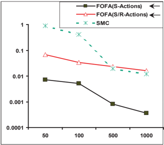
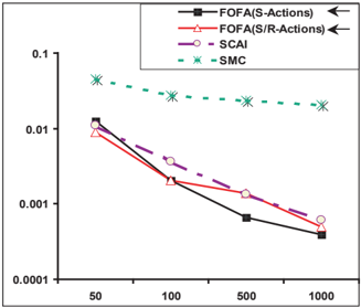
We compared the accuracy of our FOFA ( S/R-Actions ) and FOFA ( S-Actions ) with SCAI [8] and SMC algorithms. Note that we grounded the domains for running SCAI and SMC. We ran sampling algorithms (50 times) for a fixed number of samples and computed the KL-distance between their approximation and the exact posterior. We calculated the average over these derived KL-distances to approximate the expected KL-distance. SCAI assumes that deterministic actions are always executable. We include this assumption in the depots domain in which we compared the results with SCAI. In the briefcase domain, we just compared our algorithms with the SMC techniques.

Figures 7 and 8 show the expected KL-distances (in logarithmic scale) vs. number of samples in the depots and briefcase , respectively. As we expected, the average KLdistance for FOFA ( S-Actions ) is always the lowest. We expect to get more improvement when there are more objects in the domain (here, we just use 5 constants to be able to compute the exact distribution). For the briefcase domain (Figure 8) SMC has higher accuracy than FOFA ( S/R-Actions ) for 1000 samples. The reason is that the posterior distribution converges to the stationary distribution in this domain (4 constants, 256 states). Even grounded domain is not too big, but for cases involving longer sequences and more states we did not have the exact posterior to compare with since the implementation for the exact algorithm crashes.

2 Also available from: ftp://ftp.cs.yale.edu/pub/ mcdermott/domains/ .

5 Conclusions and Future Work

In this paper we presented a sampling algorithm to compute the posterior probability of a query given a sequence of actions and observations in a FO dynamic system. Our algorithm takes advantage of a compact representation and achieves higher accuracy than SMC sampling and earlier propositional sampling techniques.

There are several directions that we can continue this work: (1) Apply sampling in FO Markov Decision Processes(MDP)s [2](2) Learn the transition model in PRAM. (3) Apply the algorithm in text understanding. (4) Generalize the representation to continuous domains (e.g., by discretizing the real value variables or by combining with Rao-Blackwellised Particle Filtering [6]).

Acknowledgements

We would like to thank the anonymous reviewers for their helpful comments. This work was supported by DARPA SRI 27-001253 (PLATO project), NSF CAREER 05-46663, and UIUC/NCSA AESIS 251024 grants.

References

1. F. Bacchus, J. Y. Halpern, and H. J. Levesque. Reasoning about noisy sensors and effectors in the situation calculus. AI , 1999.
2. C. Boutilier, R. Reiter, and B. Price. Symbolic dynamic programming for first-order MDPs. In IJCAI , 2001.
3. V. S. Costa, D. Page, M. Qazi, and J. Cussens. Clp(bn): Constraint logic programming for probabilistic knowledge. In UAI , 2003.
4. T. Dean and K. Kanazawa. Probabilistic temporal reasoning. In AAAI , 1988.
5. A. Doucet, N. de Freitas, and N. Gordon. Sequential Monte Carlo Methods in Practice . Springer, 1st edition, 2001.
6. A. Doucet, N. de Freitas, K. Murphy, and S. Russell. Raoblackwellised particle filtering for dynamic bayesian networks. In UAI , 2000.
7. N. Friedman, L. Getoor, D. Koller, and A. Pfeffer. Learning probabilistic relational models. In IJCAI , 1999.
8. H. Hajishirzi and E. Amir. Stochastic filtering in a probabilistic action model. In AAAI'07 , 2007.
9. Michael Jordan. Introduction to probabilistic graphical models . 2007. Forthcoming.
10. K. Kersting, L. D. Raedt, and T. Raiko. Logical hidden markov models. Artificial Intelligence Research , 2006.
11. U. Kjaerulff. A computational scheme for reasoning in dynamic probabilistic networks. In UAI , 1992.
12. S. Muggleton. Stochastic logic programs. In Workshop on ILP , 1995.
13. Kevin Murphy. Dynamic Bayesian Networks: Representation, Inference and Learning . PhD thesis, 2002.
14. M. Nance, A. Vogel, and E. Amir. Reasoning about partially observed actions. In AAAI , 2006.
15. D. Pool. Probabilistic horn abduction and bayesian networks. Artificial Intelligence , 64:81-129, 1993.
16. L. R. Rabiner. A tutorial on hidden Markov models and selected applications in speech recognition. IEEE , 1989.
17. R. Reiter. Knowledge In Action . MIT Press, 2001.
18. Matthew Richardson and Pedro Domingos. Markov logic networks. Machine Learning , 2006.
19. A. Shirazi and E. Amir. First order logical filtering. In IJCAI , 2005.
20. B. Taskar, P. Abbeel, and D. Koller. Discriminative probabilistic models for relational data. In UAI'02 , 2002.
21. M. Welling, I. Porteous, and E. Bart. Infinite state bayesian networks. In NIPS , 2007.
22. L. S. Zettlemoyer, H. M. Pasula, and L. P. Kaelbling. Logical particle filtering. In Dagstuhl Seminar on Probabilistic, Logical, and Relational Learning , 2007.