Solving the Resource Constrained Project Scheduling Problem with Generalized Precedences by Lazy Clause Generation

Andreas Schutt †

Thibaut Feydy † Mark G. Wallace glyph[star]

Peter J. Stuckey †

† National ICT Australia, Department of Computer Science & Software Engineering, The University of Melbourne, Victoria 3010, Australia { aschutt,tfeydy,pjs } @csse.unimelb.edu.au glyph[star]

Faculty of Information Technology, Monash University, Clayton, Vic 3800, Australia [email protected]

Abstract

The technical report presents a generic exact solution approach for minimizing the project duration of the resource-constrained project scheduling problem with generalized precedences ( Rcpsp /max). The approach uses lazy clause generation, i.e., a hybrid of finite domain and Boolean satisfiability solving, in order to apply nogood learning and conflict-driven search on the solution generation. Our experiments show the benefit of lazy clause generation for finding an optimal solutions and proving its optimality in comparison to other state-of-the-art exact and non-exact methods. The method is highly robust: it matched or bettered the best known results on all of the 2340 instances we examined except 3, according to the currently available data on the PSPLib. Of the 631 open instances in this set it closed 573 and improved the bounds of 51 of the remaining 58 instances.

1. Introduction

The Resource-constrained Project Scheduling Problem with generalized precedences ( Rcpsp /max) 1 consists of scarce resources, activities and precedence constraints between pairs of activities. Each activity requires some units of resources during their execution. The aim is to build a schedule that obeys the resource and precedence constraints. Here, we concentrate on renewable resources (i.e., their supply is constant during the planning period), non-preemptive activities (i.e. once started their execution

1 In the literature Rcpsp /max is also called as Rcpsp with temporal precedences, arbitrary precedences, minimal and maximal time lags, and time windows.

cannot be interrupted), and finding a schedule that minimizes the project duration (also called makespan ). This problem is denoted as PS | temp | C max by Brucker et al. [8] and m, 1 | gpr | C max by Herroelen et al. [16]. Bartusch et al. [5] show that the decision wether an instance is feasible or not is already NP-hard.

The Rcpsp /max problem is widely studied and some of its applications can be found in Bartusch et al. [5]. A problem instance consists of a set of resources, a set of activities, and a set of generalized precedences between activities. Each resource is characterized by its discrete capacity, and each activity by its discrete processing time (duration) and its resource requirements. Generalized precedences express relations of start-to-start, start-to-end, end- to-start, and end-to-end times between pairs of activities. All these relations can be formulated as start-to-start times precedence. Those precedences have the form S i + d ij ≤ S j where S i and S j are the start times of the activities i and j resp., and d ij is a discrete distance between them. If d ij is non-negative this imposes a minimal time lag, while if d ij is negative this imposes a maximal time lag between start times.

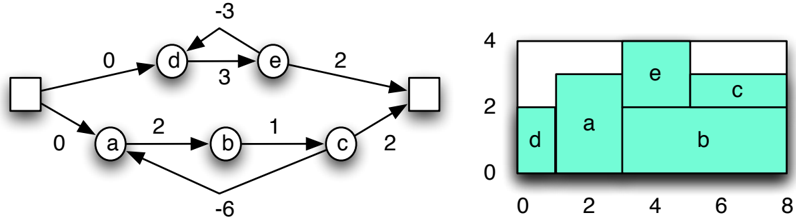
Example 1. A simple example of an Rcpsp /max problem consists of the five activities [ a, b, c, d, e ] with their start times [ s a , s b , s c , s d , s e ], their durations [2 , 5 , 3 , 1 , 2] and resource requirements on a single resource [3 , 2 , 1 , 2 , 2] and a resource capacity of 4. Suppose we also have the generalized precedences s a + 2 ≤ s b (activity a ends before activity b starts), s b + 1 ≤ s c (activity b starts at least 1 time unit before activity c starts), s c -6 ≤ s a (activity c can not start later than 6 time units after activity a starts), s d +3 ≤ s e (activity d starts at least 3 time units before activity e starts), and s e -3 ≤ s d (activity e can not start later than 3 time units after activity d starts). Note that the last two precedences express the relation s d +3 = s e (activity d starts exactly 3 time units before activity e ).

Let the planning horizon, in which all activities must be completed be 8. Figure 1 illustrates the precedence graph between the five tasks and source at the left (time 0) and sink at the right (time 8), as well as a potential solution to this problem, where a rectangle for activity i has width equal to its duration and height equal to its resource requirements. ✷

To our knowledge the first exact method to tackle Rcpsp /max was proposed by Bartusch et al. [5]. They use a branch-and-bound algorithm to tackle the problem. Their branching is based on resolving (minimal) conflict sets 2 by the addition of precedence constraints breaking these sets. Later other branch-and-bound methods were developed which are based on the same idea (e.g. De Reyck and Herreolen [10], Schwindt [29], and Fest et al. [12]). The results from Schwindt are the best published one for an exact method on the testset Sm so far.

Dorndorf et al. [11] use a time-oriented branch-and-bound combined with constraint propagation for precedence and resource constraints. In every branch one unscheduled and 'eligible' activity is selected and its start time is assigned to the earliest point in

2 Conflict sets are set of activities for which their execution might overlap in time and violate at least one resource constraint if they are executed at the same time.

time that does not violate any constraint regarding the current partial schedule. In the case of backtracking they apply dominance rules to fathom search space. As far as we can determine this exact approach outperforms other exact methods for Rcpsp /max on the CD benchmark set.

Franck et al. [15] compare different solution methods on a benchmark set UBO with instances ranging from 10 to 1000 activities. Their methods are a truncated branch-andbound algorithms, filter-beam search, heuristics with priority rules, genetic algorithms and tabu search. All methods share a preprocessing step to determining feasibility or infeasibility. The preprocessing step decomposes the precedence network into strongly connected components (SCCs) (which are denoted 'cyclic structures' in [15]). The preprocessing then determines a solution or infeasibility for each SCC individually using constraint propagation and a destructive lower bound computation. Once a solution for all SCCs is determined a first solution can be deterministically generated for the original instance; otherwise infeasibility is proven.

Ballest´ ın et al. [4] employ an evolutionary algorithm based on a serial generation scheme with unscheduling step. Their crossover operator is based on so called conglomerates , i.e. set of cycle structures and other activities which cannot move freely inside a schedule, it tries to keep the 'good' conglomerates of the parents to their children. This is the best published local search method so far on the testsets UBO (up to instances with 100 activties) and CD .

Cesta at al. [9] propose a two layered heuristic that is based on a temporal precedence network and extension of this network by new temporal precedence in order to resolve minimal conflict sets. For guidance, constraint propagation algorithms are applied on the network. Their method is competitive on the benchmark set SM .

Oddi and Rasconi [23] apply a generic iterative search consisting of of a relaxation and flatting step based on temporal precedences which are used for resolving resource conflicts. In the first step some of the temporal precedences are removed from the problem and then in the second others added if a resource conflict exists. Their methods is evaluate on instances with 200 activities from the benchmark set UBO .

Aspecial case of Rcpsp /max is the well-studied Resource-constrained Project Scheduling Problem ( Rcpsp ) where the precedence constraints S i + d ij ≤ S j express that the

activity j must start after the end of i , i.e. d ij equals to the duration of i . In contrast to Rcpsp /max the decision variant of Rcpsp is polynomial solvable, but not its optimization variant which is NP-hard (Blazewicz et al. [7]). The reason for this is the absence of maximal time lags, i.e. here activity executions can always be delayed until to a point in time where enough resource units are available without breaking any precedence constraints. That is not possible for Rcpsp /max.

The best exact methods for Rcpsp to our knowledge are our own [26, 27] and Horbach [17]. Both use advanced SAT technology in order to take advantage of its nogood learning facilities. Our methods [26, 27] are a generic approach based on the Lazy Clause Generation (LCG) [24] using the G12 Constraint Programming Platform [32]. Lazy clause generation is a hybrid of a finite domain and a Boolean satisfiability solver. Our approaches model the cumulative resource constraint either by decomposing into smaller primitive constraints, or by the creating a global cumulative propagator. The global propagation approach performs better as the size of the problem grows. In contrast to our methods Horbach's approach is a hand-tailored for Rcpsp , but similarly a hybrid with SAT solving. He uses a linear programming solver to determine activity schedules and hybridize with the SAT solver. Overall our global approach [27] is superior to Horbach's approach on Rcpsp .

In this paper we apply the same generic lazy clause generation approach to the more general problem of Rcpsp /max. Because the problems are more difficult than pure RCPSP we need to modify our approach in particular to prove feasibility/infeasibility We show that the approach to solving Rcpsp /max performs better than published methods so far, especially for improving a solution, once a solution is found, and proving optimality. We state the limitations of our current model and how to overcome them. We compare out approach to the best known approaches to Rcpsp /max on several benchmark suites accessible via the PSPLib [1].

The paper is organized as follows. In Section 2 we give an introduction to lazy clause generation. In Section 3 we present our basic model for Rcpsp /max and discuss some improvements to it. In Section 4 we discuss the various branch-and-bound procedures that we use to search for optimal solutions. In Section 5 we compare our algorithm to the best approaches we are aware of on 3 challenging benchmark suites. Finally in Section 6 we conclude.

2. Preliminaries

In this section we explain lazy clause generation by first introducing finite domain propagation and DPLL based SAT solving, and then explaining the hybrid approach. We discuss how the hybrid explains conflicts and briefly discuss how a cumulative propagator is extended to explain its propagations.

2.1. Finite Domain Propagation

Finite domain propagation (see e.g. [25]) is a powerful approach to tackling combinatorial problems. A finite domain problem ( C , D ) consists of a set of constraints C over a set

of variables V , a domain D which determine the finite set of possible values of each variable in V . A domain D is a complete mapping from V to finite sets of integers. Hence given domain D , then D ( x ) is the set of possible values that variable x can take. Let min D ( x ) = min( D ( x )) and max D ( x ) = max( D ( x )). Let [ l .. u ] = { d | l ≤ d ≤ u, d ∈ Z } denote a range of integers., where [ l .. u ] = ∅ if l > u . In this paper we will concentrate on domains where D ( x ) is a range for all x ∈ V . The initial domain is referred as D init . Let D 1 and D 2 be domains, then D 1 is stronger than D 2 , written D 1 glyph[subsetsqequal] D 2 , if D 1 ( v ) ⊆ D 2 ( v ) for all v ∈ V . Similarly if D 1 glyph[subsetsqequal] D 2 then D 2 is weaker than D 1 . For instance, all domains D that occur will be stronger than the initial domain, i.e. D glyph[subsetsqequal] D init .

A valuation θ is a mapping of variables to values, written { x 1 ↦→ d 1 , . . . , x n ↦→ d n } . We extend the valuation θ to map expressions or constraints involving the variables in the natural way. Let vars be the function that returns the set of variables appearing in an expression, constraint or valuation. In an abuse of notation, we define a valuation θ to be an element of a domain D , written θ ∈ D , if θ ( v ) ∈ D ( v ) for all v ∈ vars ( θ ). Define a valuation domain D as one where | D ( v ) | = 1 , ∀ v ∈ V . We can define the corresponding valuation θ D for a valuation domain D as { v ↦→ d | D ( v ) = { d } , v ∈ V} .

Then a constraint c ∈ C is a set of valuations over vars ( c ) which give the allowable values for a set of variables. In FD solvers constraints are implemented by propagators. A propagator f implementing c is a monotonically decreasing function on domains such that for all domains D glyph[subsetsqequal] D init : f ( D ) glyph[subsetsqequal] D and no solutions are lost, i.e. { θ ∈ D | θ ∈ c } = { θ ∈ f ( D ) | θ ∈ c } . We assume each propagator f is checking , that is if D is a valuation domain then f ( D ) = D iff θ D restricted to vars ( c ) is a solution of c . Given a set of constraints C we assume a corresponding set of propagators F = { f | c ∈ C , f implements c } .

A propagation solver for a set of propagators F and current domain D , solv ( F, D ), repeatedly applies all the propagators in F starting from domain D until there is no further change in resulting domain. solv ( F, D ) is the weakest domain D ′ glyph[subsetsqequal] D which is a fixpoint (i.e. f ( D ′ ) = D ′ ) for all f ∈ F .

glyph[negationslash]

Finite domain solving interleaves propagation with search decisions. Given a initial problem ( C , D ) where F are the propagators for the constraints C we first run the propagation solver D ′ = solv ( F, D ). If this determines failure then the problem has no solution and we backtrack to visit the next unexplored choice. If D is a valuation domain we have determined a solution. Otherwise we pick a variable x ∈ V and split its domain D ′ ( x ) into two disjoint parts S 1 ∪ S 2 = D ′ ( x ) creating two subproblems ( C , D 1 ), ( C , D 2 ), where D i ( x ) = S i and D i ( v ) = D ′ ( v ) , v = x , whose solutions are the solutions of the original problem. We then recursively explore the first problem, and when we have shown it has no solutions we explore the second problem.

As defined above finite domain propagation is only applicable to satisfaction problems . Finite domain solvers solve optimization problems by mapping them to repeated satisfaction problems. Given an objective function o to minimize under constraints C with domain D , the finite domain solving approach first finds a solution θ to ( C , D ), and then finds a solution to ( C ∪{ o ≤ θ ( o ) } , D ), that is, the satisfaction problem of finding a better solution than previously founds. It repeats this process until a problem is reached with no solution, in which case the last found solution is optimal. If the process is halted

before proving optimality, then the solving process just returns the last solution found as the best known.

Finite domain propagation is a powerful generic approach to solving combinatorial optimization problems. Its chief strengths are the ability to model problems at a very high level, and the use of global propagators, specialized propagation algorithms for important constraints.

2.1.1. Cumulative

Of particular interest to us in this work is the global cumulative constraint for cumulative resource scheduling.

The cumulative constraint introduced by Aggoun and Beldiceanu [3] in 1993 is a constraint with Zinc [20] type

predicate cumulative(list of var int: s, list of int: d, list of int: r, int: c);

Each of the first three arguments are lists of the same length n and indicate information about a set of activities . s [ i ] is the variable start time of the i th activity, d [ i ] is the fixed duration of the i th activity, and r [ i ] is the fixed resource usage (per time unit) of the i th activity. The last argument c is the fixed resource capacity .

The cumulative constraints represent cumulative resources with a constant capacity over the considered planning horizon applied to non-preemptive activities, i.e. if they are started they cannot be interrupted. Without loss of generality we assume that all values are integral and non-negative and there is a planning horizon t max which is the latest time any activity can finish.

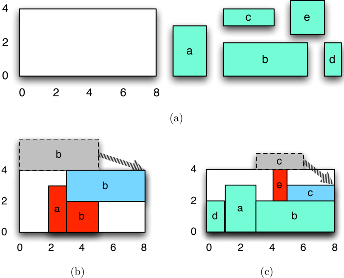
Example 2. Consider the five activities [ a, b, c, d, e ] from Example 1 with durations [2 , 5 , 3 , 1 , 2] and resource requirements [3 , 2 , 1 , 2 , 2] and a resource capacity of 4. This is represented by the cumulative constraint.

cumulative ([ s a , s b , s c , s d , s e ] , [2 , 5 , 3 , 1 , 2] , [3 , 2 , 1 , 2 , 2] . 4)

Imagine each task must start at time 0 or after and finish before time 8. The cumulative problem corresponds to packing the rectangles shown in Figure 2(a) into the resource box shown below. ✷

There are many propagation algorithms for cumulative , but the most widely used is based on timetable propagation [19]. An activity i has a compulsory part given domain D from [max D s [ i ] .. min D s [ i ]+ d [ i ] -1], that requires that activity i makes us of r [ i ] resources at each of the times in [ max D s [ i ] .. min D s [ i ] + d [ i ] -1 ] if the range is non-empty. The timetable propagator for cumulative first determines the resource usage profile ru [ t ] which sums for each time t the resources requires for all compulsory parts of activities at that time. If at some time t the profile exceeds the resource capacity, i.e. ru [ t ] > c , the constraint is violated and failure detected. If at some time t point the resource used in the profile that there is not enough left for an activity i , i.e. ru [ t ] + r [ i ] > c ,

then we can determine that activity i cannot be scheduled to run during time t . If the earliest start time of activity i , min D s [ i ] means that the activity cannot be scheduled completely before time t , i.e. min D s [ i ] + d [ i ] > t , we can update the earliest start time to be t + 1, similarly if the lastest start time of the activity means that the activity cannot be scheduled completely after t , i.e. max D s [ i ] ≤ t then we can update the latest start time to be t -d [ i ]. For a full description of timetable propagation for cumulative see e.g. [27].

Example 3. Consider the cumulative constraint of Example 2 where the domains of the start times are now D ( s a ) = [ 1 .. 2 ], D ( s b ) = [ 0 .. 3 ], D ( s c ) = [ 3 .. 5 ], D ( s d ) = [ 0 .. 2 ], D ( s e ) = [0 .. 4 ]. Then there is compulsory parts of activities a and b in the ranges [2 .. 2] and [3 .. 4] respectively shown in Figure 2(b) in red. No other activities have a compulsory part. Hence the red contour illustrates the resource usage profile. Since activity b cannot be scheduled in parallel with activity a , and the earliest start time of activity b , 0, means that the activity cannot be scheduled before activity a we can reduce the domain of the start time for activity b to the singleton [ 3 .. 3 ]. This is illustrated in Figure 2(b). The opposite holds for activity a that cannot be run after activity b , hence the domain of its start time shrinks to the singleton range [ 1 .. 1 ]. Once we make these changes the compulsory parts of the activities a and b increase to the ranges [ 1 .. 2 ] and

[ 3 .. 7 ] respectively. This in turn causes the start times of activities d and e to become [ 0 .. 0 ] and [ 3 .. 4 ] respectively creating compulsory parts in the ranges [ 0 .. 0 ] and [ 4 .. 4 ] respectively. The later causes the start time of activity c to become fixed at 5 generating the compulsory part in [ 5 .. 7 ] which causes that the start time of activity e becomes fixed at 3. This is illustrated in Figure 2(c). In this case the timetable propagation results in a final schedule in the right of Figure 1. ✷

2.2. Boolean Satisfiability

Let B be a set of Boolean variables. A literal l is Boolean variable b ∈ B or its negation ¬ b . The negation of a literal ¬ l is defined as ¬ b if l = b and b if l ≡ ¬ b . A clause C is a set of Boolean variables understood as a disjunction. Hence clause { l 1 , . . . , l n } is satisfied if at least one literal l i is true. An assignment A is a set of Boolean literals that does not include a variable and its negation, i.e. glyph[notexistential] b ∈ B . { b, ¬ b } ⊆ A . An assignment can be seen as a partial valuation on Boolean variables, { b ↦→ true | b ∈ A } ∪ { b ↦→ false |¬ b ∈ A } . A theory T is a set of clauses. A SAT problem ( T, A ) consists of a set of clauses T and an assignment over (some of) the variables occuring in T .

A Davis-Putnam-Loveland-Logemann (DPLL) SAT solver is a form of finite domain propation solver specialized for Boolean clauses. Each clause is propagated by so called unit propagation . Given an assignment A , unit propagation detects failure using clause C is such that {¬ l | l ∈ C } ⊆ A , and unit propagation detects a new unit consequence l if C ≡ { l }∪ C ′ and {¬ l ′ | l ′ ∈ C ′ } ⊆ A , in which case it adds l to the current assignment A . Unit propagation continues until failure is detected, or no new unit consequences can be determined.

SAT solvers exhaustively apply unit propagation to the current assignment A to generate all the consequences possible A ′ . They then choose an unfixed Boolean variable b and create two equivalent problem ( T, A ′ ∪ { b } ), ( T, A ′ ∪ {¬ b } ) and recursively search these subproblems. The Boolean literals added to the assignment by choice are termed decision literals .

Modern DPLL based SAT solving is a powerful approach to solving combinatorial optimization problems because it records nogoods that prevent the search from revisiting similar parts of the search space. The SAT solver records an explanation for each unit consequence discovered (the clause that caused unit propagation), and on failure uses these explanations to determine a set of mutually incompatible decisions, a nogood which is added as a new clause to the theory of the problem. These nogoods drastically reduce the size of the search space needed to be examined. Another advantage of SAT solvers is that they track which Boolean variables are involved in the most failures (called active variables), and use a powerful autonomous search procedure which concentrates on the variables that are most active. The disadvantages of SAT solvers are the restriction to Boolean variables and the sometime huge models that are required to represent a problem because the only constraints expressible are clauses.

2.3. Lazy Clause Generation

Lazy clause generation is a hybrid of finite domain propagation and Boolean satisfiability. The key idea in lazy clause generation is to run a finite domain propagation solver, but to build explanation of the propagations made by the solver by recording them as clauses on a Boolean variable representation of the problem. Hence as the FD search progresses we lazily create a clausal representation of the problem. The hybrid has the advantages of FD solving, but inherits the SAT solvers ability to create nogoods to drastically reduce search, and use activity based search.

2.3.1. Variable Representation

In lazy clause generation each integer variable x ∈ V with the initial domain D init = [ l .. u ] is represented by the following Boolean variables J x = l K , . . . , J x = u K and J x ≤ l K , . . . , J x ≤ u -1 K . The variable J x = d K is true if x takes the value d , and false if x takes a value different from d . Similarly the variable J x ≤ d K is true if x takes a value less than or equal to d and false for a value greater than d . Note that we use J x = d K and J x ≤ d K throughout the paper as the names of Boolean variables. Sometimes the notation d ≤ x is used for the literal ¬ x ≤ d -1 .

J K J K Not every assignment of Boolean variables is consistent with the integer variable x , for example { J x = 3 K , J x ≤ 2 K } (i.e. both Boolean variables are true) requires that x is both 3 and ≤ 2. In order to ensure that assignments represent a consistent set of possibilities for the integer variable x we add to the SAT solver the clauses DOM ( x ) that encode J x ≤ d K → J x ≤ d + 1 K , l ≤ d < u , J x = l K ↔ J x ≤ l K , J x = d K ↔ ( J x ≤ d K ∧¬ J x ≤ d -1 K ) , l < d < u , and J x = u K ↔¬ J x ≤ u -1 K where D init ( x ) = [ l .. u ]. We let DOM = ∪{ DOM ( v ) | v ∈ V} .

Any assignment A on these Boolean variables can be converted to a domain: domain ( A )( x ) = { d ∈ D init ( x ) | ∀ J c K ∈ A,vars ( J c K ) = { x } : x = d | = c } , that is, the domain includes all values for x that are consistent with all the Boolean variables related to x . It should be noted that the domain may assign no values to some variable.

Example 4. Consider Example 1 and assume D init ( s i ) = [ 0 .. 15 ] for i ∈ { a, b, c, d, e } . The assignment A = {¬ J s a ≤ 1 K , ¬ J s a = 3 K , ¬ J s a = 4 K , J s a ≤ 6 K , ¬ J s b ≤ 2 K , J s b ≤ 5 K , ¬ J s c ≤ 4 K , J s c ≤ 7 K , ¬ J s e ≤ 3 K } is consistent with s a = 2, s a = 5, and s a = 6. Hence domain ( A )( s a ) = { 2 , 5 , 6 } . For the remaining variables domain ( A )( s b ) = [ 3 .. 5 ], domain ( A )( s c ) = [5 .. 7 ], domain ( A )( s d ) = [0 .. 15 ], and domain ( A )( s e ) = [4 .. 15 ]. Note that for brevity A is not a fixpoint of a SAT propagator for DOM ( s a ) since we are missing many implied literals such as ¬ J s a = 0 K , ¬ J s a = 8 K , ¬ J s a ≤ 0 K etc. ✷

2.3.2. Explaining Propagators

In LCG a propagator is extended from a mapping from domains to domains to a generator of clauses describing propagation. When f ( D ) = D we assume the propagator f can determine a clause C to explain each domain change. Similarly when f ( D ) is a false domain the propagator must create a clause C that explains the failure.

glyph[negationslash]

Example 5. Consider the propagator f for the precedence constraint s a +2 ≤ s b from Example 1. When applied to the domains D ( s i ) = [0 .. 15 ] for i ∈ { a, b } it obtains f ( D )( s a ) = [ 0 .. 13 ], and f ( D )( s b ) = [ 2 .. 13 ]. The clausal explanation of the change in domain of s a is J s b ≤ 15 K → J s a ≤ 13 K , similarly the change in domain of s b is ¬ J s a ≤ -1 K → ¬ J s b ≤ 1 K ( J s a ≥ 0 K → J s b ≥ 2 K ). These become the clauses ¬ J s b ≤ 15 K ∨ J s a ≤ 13 K and J s a ≤ -1 K ∨ ¬ J s b ≤ 1 K . ✷

The explaining clauses of the propagation are added to the database of the SAT solver on which unit propagation is performed. Because the clauses will always have the form C → l where C is a conjunction of literals true in the current assignment, and l is a literal not true in the current assignmet, the newly added clause will always cause unit propagation, adding l to the current assignment.

Example 6. Consider the propagation from Example 5. The clauses ¬ J s b ≤ 15 K ∨ J s a ≤ 13 K and J s a ≤ -1 K ∨ ¬ J s b ≤ 1 K are added to the SAT theory. Unit propagation infers that J s a ≤ 13 K = true and ¬ J s b ≤ 1 K = true since ¬ J s b ≤ 15 K and J s a ≤ -1 K are false , and adds these literals to the assignment. Note that the unit propagation is not finished, since for example the implied literal J s a ≤ 14 K , can be detected true as well. ✷

The unit propagation on the added clauses C is guaranteed to be as strong as the propagator f on the original domains, i.e. if domain ( A ) glyph[subsetsqequal] D then domain ( A ′ ) glyph[subsetsqequal] f ( D ) where A ′ is the resulting assignment after addition of C and unit propagation (see [24] for the formal results).

Note that a single new propagation may be explainable using different set of clauses. In order to get maximum benefit from the explanation we desire a 'strongest' explanation as possible. A set of clauses C 1 is stronger than a set of clauses C 2 if C 2 implies C 1 . In other words, C 1 restricts the search space at least as much as C 2 .

Example 7. Consider explaining the propagation of the start time of the activity c described in Example 3 and Figure 2(c). The domain change J 5 ≤ s c K arises from the compulsory parts of activity b and e as well as the fact that activity c cannot start before time 3. An explanation of the propagation is hence J 3 ≤ s c K ∧ J 3 ≤ s b K ∧ J s b ≤ 3 K ∧ J 3 ≤ s e ∧ s e ≤ 4 → 5 ≤ s c .

J K J K Moreover, the compulsory parts of the activity b in the ranges [ 3 .. 3 ] and [ 5 .. 7 ] are not necessary for the domain change. We only require that there is not enough resources at time 4 to schedule task c . Thus the refined explanation can be further strengthened by replacing J 3 ≤ s b K ∧ J s b ≤ 3 K by J s b ≤ 4 K which is enough to force a compusory part of s b at time 4. This leads to the stronger explanation J 2 ≤ s c K ∧ J s b ≤ 4 K ∧ J 3 ≤ s e K ∧ J s e ≤ 4 K → J 5 ≤ s c K .

K J K J K We can observe that if 2 ≤ s c then the same domain change J 5 ≤ s c K follows due to the compulsory parts of activity b and e . Therefore, a stronger explanation is obtained by replacing the literal 3 ≤ s c by 2 ≤ s c .

In this example the final explanation corresponds to a pointwise explanation in Schutt et al. [27]. Here, those pointwise explanations are used to explain the timetable propagation. For a full discussion about the best way to explain cumulative propagation see [27].

2.3.3. Nogood generation

Since all the propagation steps in lazy clause generation have been mapped to unit propagation on clauses, we can perform nogood generation just as in a SAT solver.

The nogood generation is based on an implication graph and the first unique implication point (1UIP). The graph is a directed graph where nodes represent fixed literals and directed edges reasons why a literal became true , and is extended as the search progresses. Each unit propagation marks the literal it makes true with the clause that caused the unit propagation. The true literals are kept in a stack showing the order that they were determined as true by unit consequence or decisions.

For clarity purpose, we do not differentiate between literal and node. A literal is fixed either by a search decision or unit propagation. In the first case the graph is extended only by the literal and in the second case by the literal and incoming edges to that literal from all other literals in the clause on that the unit propagation assigned the true value to the literal.

Example 8. Consider the strongest explanation J 2 ≤ s c K ∧ J s b ≤ 4 K ∧ J 3 ≤ s e K ∧ J s e ≤ 4 K → J 5 ≤ s c K from Example 7. It is added to the SAT database as clause ¬ J 2 ≤ s c K ∨ ¬ J s b ≤ 4 K ∨ ¬ J 3 ≤ s e K ∨ ¬ J s e ≤ 4 K ∨ J 5 ≤ s c K and unit propagation sets J 5 ≤ s c K true . Therefore the implication graph is extended by the edges J 2 ≤ s c K → J 5 ≤ s c K , J s b ≤ 4 K → J 5 ≤ s c K , J 3 ≤ s e K → J 5 ≤ s c K , and J s e ≤ 4 K → J 5 ≤ s c K . ✷

Every node and edge is associated with the search level at which they are added to the graph. Once a conflict encounters a nogood which is the 1UIP in LCG is calculated based on the implication graph. A conflict is recognized when the unit propagation reaches a clause where all literals are false. This clause is the starting point of the analysis and builds a first tentative nogood. Now, literals in the tentative nogood are replaced by the literals from its incoming edges in the reverse order of the graph extension. This process holds on until the tentative nogood includes exactly one literal from the current decision level. The resulting nogood is called 1UIP (first unique implication point), since it corresponds to a cut through the implication graph that has one node in the current decision level.

Example 9. Considered the Rcpsp /max instance from Example 1 on page 2.

Assume an initial domain of D init = [0 .. 15 ] then after the initial propagation of the precedence constraints the domains are D ( s a ) = [ 0 .. 8 ], D ( s b ) = [ 2 .. 10 ], D ( s c ) = [ 3 .. 12 ], D ( s d ) = [ 0 .. 10 ], and D ( s b ) = [ 3 .. 13 ]. Note that no tighter bounds can be inferred by the cumulative propagator.

Assume search now sets s a ≤ 0. This sets the literal J s a ≤ 0 K as true, and unit propagation on the domain clauses will set J s a = 0 K , J s a ≤ 1 K , J s a ≤ 2 K , etc. In the remainder of the example we will ignore propagation of the domain clauses and concentrate on the 'interesting propagation'.

The precedence constraint s c -6 ≤ s a will force s c ≤ 6 with explanation J s a ≤ 0 K → J s c ≤ 6 K . The the precedence constraint s b +1 ≤ s c will force s b ≤ 5 with explanation J s c ≤ 6 K → J s b ≤ 5 K .

%

%

GLYPH<30>

GLYPH<30>

'

'

8

8

[

]

'

c

'

'

f

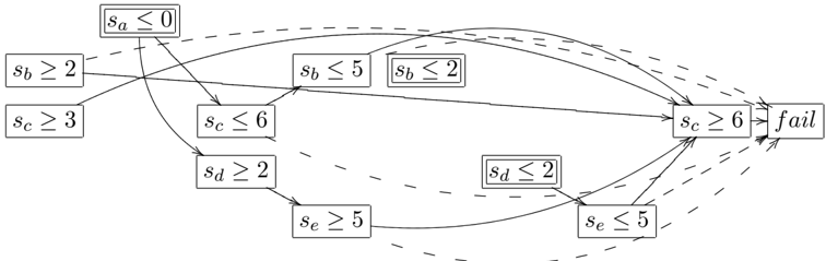
Figure 3: (Part of) The implication graph for the propagation of Example 9. Decision literals are shown double boxed, while literals set by unit propagation are shown boxed.

The timetable propagator for cumulative will use the compulsory part of activity a in [0 .. 2) to force s d ≥ 2. The explanation for this is J s a ≤ 0 K → J s d ≥ 2 K . The the precedence s d +3 ≤ s e forces s e ≥ 5 with explanation s d ≥ 2 → s e ≥ 5 .

J K J K Suppose next that search sets s b ≤ 2. There is no propagation from precedence constraints or the cumulative constraint. It does create a compulsory part of s b from [2 .. 7) but there is no propagation.

Suppose now that search sets s d ≤ 2. Then the precedence constraint s e -3 ≤ s d forces s e ≤ 5 with explanation J s d ≤ 2 K → J s e ≤ 5 K . This creates a compulsory part of d in [2 .. 3) and a compulsory part of e in [5 .. 7). In fact all the activities a , b , d and e are fixed now. Timetable propagation sees since all resources are used at time 5 then activity c cannot start before time 6. A reason for this is J s b ≥ 2 K ∧ J s b ≤ 5 K (which forces b to use 2 resources in [5..7)), plus J s e ≥ 5 K ∧ J s e ≤ 5 K (which forces e to use 2 resources in [5..7)), plus J s c ≥ 3 K (which forces c to overlap this time. Hence an explanation is s b ≥ 2 ∧ s b ≤ 5 ∧ s e ≥ 5 ∧ s e ≤ 5 ∧ s c ≥ 3 → s c ≥ 6 .

K J K The nogood generation process starts from this original explanation. It removes the last literal in the explanation by replacing it by its explanation. Replacing J s c ≥ 6 K by its explanation creates the new nogood J s b ≥ 2 K ∧ J s b ≤ 5 K ∧ J s e ≥ 5 K ∧ J s e ≤ 5 K ∧ J s c ≥ 3 K ∧ J s c ≤ 6 K → fail . Since this nogood has only one literal that was made true after the last decision level J s e ≤ 5 K this is the 1UIP nogood. Rewritten as a clause it is J s b ≤ 1 K ∨ ¬ J s b ≤ 5 K ∨ J s e ≤ 4 K ∨ ¬ J s e ≤ 5 K ∨ J s c ≤ 2 K ∨ ¬ J s c ≤ 6 K . ✷

J K J K J K J K J K J K This forces a compulsory part of c at time 6 which causes a resource overload at that time. An explanation of the failure is J s b ≥ 2 K ∧ J s b ≤ 5 K ∧ J s e ≥ 5 K ∧ J s e ≤ 5 K ∧ J s c ≥ 6 ∧ s c ≤ 6 → fail . The edges are shown in the conflict graph as dashed (for clarity).

After discovering a new nogood C the lazy clause generation solver, like a SAT solver, adds the clause C to the theory, and backtracks to the decision level of the second newest literal in nogood C . At this point we are guaranteed that the clause will unit propagate. After unit propagation finishes search proceeds as usual.

Example 10. Continuing Example 9, the solver backtracks to the decision level of the

.

.

'

'

;

;

"

"

@

@

7

7

/

/

8

8

)

)

&

&

@

@

second newest literal (in this case s e ≤ 5) thus undoing the decisions s d ≤ 2 and s b ≤ 2 and their consequences. The newly added nogood unit propagates to force s e ≥ 6 with explanation J s b ≥ 2 K ∧ J s b ≤ 5 K ∧ J s e ≥ 5 K ∧ J s c ≥ 3 K ∧ J s c ≤ 6 K → J s e ≥ 6 K , and the precedence constraint s e -3 ≤ s d forces s d ≥ 3 with explanation J s e ≥ 6 K → J s d ≥ 3 K . Search proceeds looking for a solution. ✷

3. Models for RCPSP/max

In this section a basic model for Rcpsp /max instance is presented at first, and then different possible model improvements which are mainly based on activities in disjunction.

An Rcpsp /max problem can be represented as follows: A set of activities V = { 1 , . . . , n } is subjected to generalized precedences in E ⊂ V 2 × Z between two activities, and scarce resources in R . The goal is to find a schedule S = ( S i ) i ∈V that respects the precedence and resource constraints, and minimizes the project duration (makespan) where S i is the start time of the activity i .

Each activity i has a finite processing time or duration p i and requires (non-negative) r ik units of resource k , k ∈ R for its execution where r ik is the resource requirement or usage of activity i for resource k . A resource k ∈ R has a constant 3 resource capacity R k over the planning period which cannot be exceeded at any point in time. The planning period is given by [0 , t max ) where t max is the maximal planning horizon.

Generalized precedences ( i, j, d ij ) ∈ E between the activities i and j are subjected to the constraint S i + d ij ≤ S j , i.e. it represents a minimal time lag ( j must start at least d ij time units after i starts) if d ij ≥ 0 and a maximal time lag ( i must start at most -d ij time units after the start of j ) if d ij < 0. Generalized precedences encode not only start-to-start relations between activities, but also start-to-end, end-to-start, and end-to-end by addition/ subtraction of i 's or j 's duration to d ij . If a minimal time lag d + ij and a maximal time lag d -ji exist for an activity j concerning to i then the start time S j is restricted to [ S i + d + ij ..S i -d -ji ]. In the case of d + ij = -d -ji the activity j must start exactly d + ij time units after i .

For the remainder of this section let an Rcpsp /max instance be given with activities V = { 1 , 2 , . . . , n } , generalized precedences E , resources R , and a planning period [0 , t max ). Then the basic model can be stated as the following Zinc [20] model.

%---------------------------------------------------------------------% % Parameters int: t max; % The planning horizon set of int: R; % The set of resources set of int: V; % The set of activities set of int: Idx; % The index set of precedences array [R] of int: rcap; % The resource capacities array [V] of int: p; % The activities durations

3 Variation of resource capacities can be obtained by using artificial activities that claim the not-available resource units.

array [V, R] of int: r; % The activities resource requirements array [Idx, 1..3] of int: E; % The precedences of form x + c <= y set of int: Times = 0..t max; % The planning period %---------------------------------------------------------------------% % Variables array [V] of var Times: S; var Times: objective; %---------------------------------------------------------------------% % Constraints % Precedence constraints constraint forall (id in Idx) (S[E[id, 1]] + E[id, 2] <= S[E[id, 3]]); % Cumulative resource constraints constraint forall (res in R) (cumulative(S, p, [r[i, res] | i in V], rcap[res])); % Objective constraints constraint forall (i in V) (S[i] + p[i] <= objective); %---------------------------------------------------------------------% % Search solve minimize objective; %---------------------------------------------------------------------%

This basic model has a number of weaknesses: first the initial domains of the start times are large, second each precedence constraint is modelled as one individual propagator, and finally the SAT solver in LCG has no structural information about activities in disjunction.

A smaller initial domain can be computed by taking into account the precedences in E as described in the next subsection. Individual propagators for precedences may not be so bad for a small number of precedences, but for a larger number of propagators, their queuing behaviour may result in long and costly sequences of propagation steps. A global propagator can efficiently adjust the time-bounds in O ( n log n + m ) time as described in Feydy et al. [13], but we did not have access to such a propagator for the experiments. Reified precedence constraints can be used for modelling activities in disjunctions as described later in this section.

3.1. Initial Domain

A smaller initial domain can be obtained for the start time variables by applying the Bellman-Ford single source shortest path algorithm [6, 14] on the digraph G = ( V ′ , E ′ ) where V ′ = V ∪ { v 0 , v n +1 } , E ′ = { ( i, j, -d ij ) | ( i, j, d ij ) ∈ E} ∪ { ( v 0 , i, 0) , ( i, v n +1 , -p i ) | i ∈ V} , v 0 is the source node, and v n +1 is the sink node. The digraph is referred as the activity-on-node network in the literature (e.g. [5, 22]). If the digraph contains a

negative-weight cycle then the Rcpsp /max instance is infeasible. Otherwise the shortest path from the source v 0 to an activity i determines the earliest possible start time for i , i.e. -w ( v 0 → i ) where w ( . ) is the length of the path and the shortest path from an activity i to the sink v n +1 the latest possible start time for i in any schedule, i.e. t max + w ( i → v n +1 ). The Bellman-Ford algorithm has a runtime complexity of O ( |V| × |E| ).

These earliest and latest start times can not only used for an initial smaller domain, but also to improve the objective constraints by replacing them with

% Objective constraints constraint forall (i in V) (S[i] + tail[i] <= objective);

where tail[i] is the 'negative' length -w ( i → v n +1 ) of the shortest path from i to v n +1 in the digraph G . Preliminaries experiments confirmed that this modification gave major improvements for solving an instance and generating a first solution, especially on larger instances. Another advantage specific to LCG is that a smaller initial domain also reduces the size of the problem because less Boolean variables are necessary to represent the integer domain in the SAT solver.

3.2. Activities in Disjunction

Two activities i and j ∈ V are in disjunction , if they cannot be executed at the same time, i.e. their resource requirement for at least one resource k ∈ R is bigger than the available capacity: r ik + r jk > R k . Activities in disjunction can be exploited in order to reduce the search space.

The simplest way to model two activities i and j in disjunction is by two propositional constraints sharing the same Boolean variable B ij .

If B ij is true then i must end before j starts (denoted by i glyph[lessmuch] j ), and if B ij is false then j glyph[lessmuch] i . The literals B ij and ¬ B ij can be directly represented in the SAT solver, consequently B ij represents the relation (structure) between these activities. The propagator of such a propositional constraint can only infer new bounds on left hand side of the implication if the right hand side is false, and on the start times variables if the left hand side is true. For example, the right hand side in the second constraint is false if and only if max D S i -min D S j < p j . In this case the literal ¬ B ij must be false and therefore i glyph[lessmuch] j .

Adding these redundant constraints to the model allows the propagation solver to more quickly determine information about start time variables. The Zinc model of these constraints is

% Redundant non-overlapping (disjunctive) constraints

constraint forall (i, j in V where i < j) ( if exists(res in R)(r[i, res] + r[j, res] > rcap[res]) then % Activity i must be run before or after j let { var bool: b } in ( (b -> S[i] + p[i] <= S[j]) /\ (not(b) -> S[j] + p[j] <= S[i]) ) else true endif );

The detection which activity runs before the other can be further improved by considering the domains of the start times, and the minimal distances in the activity-onnode-network (see e.g. Dorndorf et al. [11]).

4. The Branch-and-Bound Algorithm

Our branch-and-bound algorithms are based on deterministic and conflict- driven branching strategies. We use them solely or in combination as a hybrid where at first the deterministic and then the conflict-driven branching is chosen (cf. Schutt et al. [26]). After each branch all constraints are propagated until a fixpoint is reached or the inconsistency for the partial schedule or the instance is proven. In the first case a new node is explored and in the second case an unexplored branch is chosen if one exists or backtracking is performed.

4.1. Deterministic Branching

The deterministic branching strategy selects an unfixed start time variable S i with the smallest possible start time min D S i . If there is a tie between several variables then the variable with the biggest size, i.e. max D S i -min D S i , is chosen. If there is still a tie then the variable with the lowest index i is selected. The binary branching is as follows: left branch S i ≤ min D S i , and right branch S i > min D S i . We denote this branching strategy by Mslf .

This branching creates a time-oriented branch-and-bound algorithm similar to Dorndorf et al. [11], but it is simpler and does not involves any dominance rule. Hence, it is weaker than their algorithm.

4.2. Conflict-driven Branching

The conflict-driven branching is a binary branching over literals in the SAT solver. In the left branch the literal is set to true and in the right branch to false . As described in Sec. 2.3.1 on page 9 the Boolean variables in the SAT solver represent values in the integer domain of a variable x (e.g. ¬ J x ≤ 3 K ( J x ≤ 10 K )) or a disjunction between activities. Hence, it creates a branch-and-bound algorithm that can be considered as a mixture of time oriented and conflict-set oriented.

As branching heuristic the Variable-State-Independent-Decaying-Sum ( Vsids ) [21] is used which is a part of the SAT solver. In each branch it selects the literal with the highest activity counter where an activity counter is assigned to each literal, and is increased during conflict analysis if the literal is related to the conflict. The analysis results in a nogood which is added to the clause data base. Here, we use the 1UIP as a nogood.

In order to accelerate the solution finding and increase the robustness of the search on hard instances Vsids can be combined with restarts which has been shown beneficial in SAT solving. On restart the set of nogoods and the activity counter has changed, so that the search will explore a very different part of the search tree. In the remainder Vsids with restart is denoted by Restart . Different restart policies can be applied, here a geometric restart on nodes with an initial limit of 250 and a restart factor of 2 . 0 are used.

4.3. Hybrid Branching

At the beginning of each search the activity counters are all initialized with the same value which can result in a poor performance of Vsids at the start of search. In order to avoid this situation at first Mslf can be chosen for branching and then Vsids used after a restart is performed (e.g. after a specific number of explored nodes). This has the advantage that the deterministic search initializes the activity counters with more meaningful values that can be fully exploited by Vsids . Here, we switch the searches after exploration of the first 500 nodes unless otherwise stated. In the remainder we refer to the strategy as Hot Start . Once more, the Vsids search after the first restart can benefit from restart. We denote the hybrid branching approach with restarts by Hot Restart .

5. Computational Results

We carried out experiments on Rcpsp /max instances available from [2] and accessible from the PSPLib [1]. Our approach is compared to the best known exact and non-exact methods so far on each testset. At the website http://www.cs.mu.oz.au/~pjs/rcpsp detailed results can be obtained.

Our methods are evaluated on the following testsets which were systematically created using the instance generator ProGen/max (Schwindt [28]):

• CD - 1080 instances with 100 activities and 5 resources (cf. Schwindt [30]).
• UBO -ubo10 , ubo20 , ubo50 , ubo100 , and ubo200 : each containing 90 instances with 5 resources and 10, 20, 50, 100, and 200 activities respectively (cf. Franck et al. [15]).
• SM -j10 , j20 , and j30 : each containing 270 instances with 5 resources and 10, 20, and 30 activities respectively (cf. Kolisch et al. [18]).

Note that although the testset SM consists of small instances they are considerably harder than e.g. ubo10 and ubo20 .

The experiments were run on Intel(R) Xeon(R) CPU E54052 processor with 2 GHz clock running GNU/Linux. The code was written in Mercury using the G12 Constraint Programming Platform and compiled with the Mercury Compiler using grade hlc.gc.trseg. Each run was given a 10 minute runtime limit.

5.1. Setup and Table Notations

In order to solve each instance a two-phase process was used. Both phases used the basic model with the two extensions described in Subsections 3.1 and 3.2.

In the first phase a Hot Start search was run to determine a first solution or to prove the infeasibility of the instance. In contrast to the normal Hot Start we give the deterministic search more time to find a first solution and therefore we switch to Vsids only after after 5 × n nodes are explored, where n is the number of activities.

The feasibility runs were set up with the trivial upper bound on the makespan t max = ∑ i ∈V max( p i , max { d ij | ( i, j, d ij ) ∈ E} ). The first phase was run until a solution (with makespan UB ) was found or infeasibility proved or the time limit reached. In the first phase the the search strategy used should be at both finding feasible solutions and proving infeasibility. Hence, it could be exchanged with methods which might be more suitable than Hot Start .

In the second optimization phase, each feasible instance was set up again this time with t max = UB . The tighter bound is highly beneficial to lazy clause generation since it reduces the number of Boolean variables required to represent the problem. The search for optimality was performed using one of the various search strategies defined in the previous section.

The execution of the two-phased process lead to the following measurements.

• rt max : The runtime limit in seconds (for both phases together).
• rt avg : The average runtime in seconds (for both phases).
• fails: The average number of fails perfomed in both phases of the search.
• feas: The percentage of instances for which a solution was found.
• infeas: The percentage of instances for which the infeasibility was proven.
• opt: The percentage of instances for which an optimal solution was found and proven.
• ∆ LB : The average distance from the best known lower bounds of feasible instances given in [2].
• #svd: The number of instances which were proven to be infeasible or optimal.
• cmpr(i): Columns with this header give measurements only related to those instances that were solved by each procedure where i is the number of these instances.

Table 1: Comparison on the testsets CD, UBO, and SM

Procedure	#svd	∆ LB	cmpr(2230)		all(2340)
			rt avg	fails	rt avg	fails
Mslf	2237	3.96785	7.73	6804	35.96	23781
Mslf with restart	2237	3.96352	7.80	6793	36.04	23787
Vsids	2276	3.76928	2.16	1567	22.91	13211
Restart	2276	3.73334	2.02	1363	22.38	12212
Hot Start	2277	3.84003	2.22	1684	22.71	12933
Hot Restart	2278	3.73049	2.04	1475	22.36	12341

all(i): Columns with this header comare measurements for all instances examined in the experiment where i is the number of these instances.

A note about special entries in the tables. A table entry '-' indicates no related number was available from previously published work. A table entry with two numbers the second in parentheses indicates the procedure was applied several times: the first number is the average over all runs with the second number, in parentheses, is the best number for all runs. A table entry marked ' glyph[star] ' indicates the situation where a procedure was not able to find a solution for all feasible instances and therefore the corresponding number may not be comparable with the number for other procedures in the same column.

5.2. Comparison of the different strategies

In the first experiment we compare all of our search strategies against each other on all testsets. The strategies are compared in terms of rt avg and failures for each test set.

The results are summarized in the Table 1. Similar to the results for Rcpsp in Schutt et al. [27] all strategies using Vsids are superior to the deterministic methods ( Mslf ), and similarly competitive. Hot Restart is the most robust strategy, solving the most instances to optimality and having the lowest ∆ LB . Restart is essential to make the search more robust for the conflict-driven strategies, whereas the impact of restart on Mslf is minimal.

In contrast to the results in Schutt et al. [27] for Rcpsp the conflict-driven searches were not uniformly superior to Mslf . The three instances 67, 68, and 154 from j30 were solved to optimality by Mslf and Mslf with restart, but neither Restart and Hot Restart could prove the optimality in the given time limit, whereas Vsids and Hot Start were not even able to find an optimal solution within the time limit. Furthermore, our method could not find a first solution for the ubo200 instances 2, 4, and 70 nor prove the infeasibility for the ubo200 instance 40 within 10 minutes.

5.3. Results on the testset CD

Table 2 presents the results for the testsets CD where 98 . 1% (1 . 9%) of the instances are feasible (infeasible). Here, we compare Restart and Hot Restart with the time-

Table 2: Results on the testset CD

Procedure	rt max	rt avg	feas	opt	infeas	∆ LB
B&B D00	100	-	98.1	71.7	1.9	4 . 6 a
Eva	-	0.62	98.1	≥ 65 . 9	-	3.24 (3.16)
Restart	1	0.38	97.9	78.1	1.6	4.73 glyph[star]
	10	1.39	98.1	89.8	1.9	3.20
	100	6.17	98.1	94.0	1.9	2.86
	600	19.32	98.1	95.8	1.9	2.81
Hot Restart	1	0.44	97.9	76.8	1.6	4.87 glyph[star]
	10	1.49	98.1	89.6	1.9	3.20
	100	6.27	98.1	93.9	1.9	2.86
	600	19.42	98.1	96.0	1.9	2.79

a ∆ LB is based on the lower bounds presented in Schwindt [30] which were not accessible for us.

oriented branch-and-bound procedure (B&B D00 ) from Dorndorf et al. [11] and the evolutionary algorithm Eva from Ballest´ ın et al. [4]. The method B&B D00 performs better on this testset than the methods proposed by De Reyck and Herroelen [10], Schwindt [29] 4 , and Fest et al. [12]. Moreover, B&B D00 is the best published exact method on this testset so far. The B&B D00 method was implemented in C++ using Ilog Solver and Ilog Scheduler . Their experiments were run on a Pentium Pro/200 PC with NT 4.0 as operating system, thus their results were obtained on a machine approximately ten times slower.

We compare our results achieved with a runtime limit of 1 second to their results with a limit of 100 seconds which should be clearly in favour of them. While B&B D00 can prove feasibility and infeasibility of all instances, the first-phase Hot Start search with one second was unable to prove infeasibilty of four infeasible instances or find solutions to two feasible instances. It does prove infeasibility of these four infeasible instances in less than 2 . 1 seconds and finds a first solution for these two feasible instances in 4 . 8 seconds and 5 . 04 seconds respectively. Within one second both our methods Restart and Hot Restart were able to prove the optimality of substantially more instances than B&B D00 . With more time our methods are able to prove optimality of almost all instances in these testsets.

One reason for the first-phase results at one second may simply be that there is a reasonable set up time required for lazy clause generation to generate all the Boolean variables and hence there is not much time left for search. Another reason for the weakness of proving infeasibility is that our model only contains propagators that determine the order of activities in disjunction concerning their domains, but not also their minimal distance in the transitive closure of all precedences. 5 Dorndorf et al. [11] shows that these propagators are crucial for detecting infeasibility. That Hot Start is not so good

4 As reported in [11]

5 The missing propagators are not available in the G12 Constraint Programming Platform.

Table 3: Results on the testset UBO for ubo10 , ubo20 , ubo50 and ubo100 instances in comparison with Franck et al.

Procedure	rt max	rt avg	feas + infeas	feas	opt	infeas	∆ LB
Fbs F01	n	12.4	99.66	-	-	-	6 . 82 glyph[star]
Dm F01	n	0.03	100	81.7	-	18.3	10 . 72
Ga F01	n	3.16	100	81.7	-	18.3	6 . 93
Restart	n/ 100	0.21	95.0	80.0	70.8	15.0	5.73 glyph[star]
	n/ 10	0.78	100	81.7	75.3	18.3	4.99
Hot Restart	n/ 100	0.25	95.0	80.0	69.7	15.0	5.73 glyph[star]
	n/ 10	0.81	100	81.7	75.3	18.3	5.04

at finding a first solution is not surprising, since the search is not very problem specific as B&B D00 . In order to overcome these problems one could run at first e.g. B&B D00 to prove infeasibility and generate a first solution, and then apply our methods.

The method Eva is the best published local search procedure on this testset. Their results were obtained on a Samsung X15 Plus computer with Pentium M processor with 1400 MHz clock speed. This means that our machine is about 1.46 times faster than their. Their limits are a maximum of 5000 schedules and a stop of the process if within 10 generation the best schedule could not be improved. Our methods generates better schedules within 10 seconds than there approach, visible in the lower ∆ LB of 3.20.

Overall our methods are able to close 310 open problems and improve the upper bound for all 21 remaining open problems in testset CD, according to the results recorded in [2].

5.4. Results on testset UBO

Table 3 compares our procedures Restart and Hot Restart with the truncated branch-and-bound methods Fbs F01 , the heuristic Dm F01 , and the genetic algorithm Ga F01 all proposed by Franck et al. [15] on the UBO testset where 81 . 7% (18 . 3%) of the instances are feasible (infeasible). In this table we add the column feas + infeas showing the sum of percentage of feas and infeas because the corresponding numbers for Fbs F01 are not available. Their results were obtained on personal computer PII with a 333MHz processor running NT 4.0 as operating system, i.e. our machine is about 6.2 times faster. They imposed a time limit of n seconds, e.g. an instance with 100 activities was given at most 100 seconds. We compare our methods with 10 (100) times lower time limit which should be favorable to the other methods.

Their methods were able to prove the feasibility or infeasibility for all instances (except one instance for the method Fbs F01 ). Indeed Dm F01 is extremely fast requiring just 0.03 seconds on average, but it does not necessarily find very good solutions, as shown by the high ∆ LB .

In contrast our first-phase was not always able to find a first solution or prove infeasibilty with the time limit n/ 100. No solution was found for 6 instances with 100 activities and the infeasibility was not shown for 11 (1) instances with 100 (50) activities. Once the time limit was extended to n/ 10 then the first phase was always able to find a solution

Table 4: Results on the testset UBO for ubo10 , ubo20 , ubo50 and ubo100 instances in comparison with Ballest´ ın et al.

Procedure	rt max	rt avg	feas	opt	infeas	∆ LB
Eva	-	0.38	81.7	-	-	4.82 (4.79)
Restart	1	0.22	80.0	71.4	15.3	5.60 glyph[star]
	10	0.89	81.7	75.3	18.3	4.92
	100	5.32	81.7	77.2	18.3	4.51
	600	24.47	81.7	78.1	18.3	4.40
Hot Restart	1	0.26	80.0	70.6	15.3	5.65 glyph[star]
	10	0.92	81.7	75.3	18.3	5.01
	100	5.26	81.7	77.2	18.3	4.55
	600	24.14	81.7	78.1	18.3	4.43

Table 5: Results on the testset UBO for ubo200 instances

Procedure	rt max	rt avg	feas	opt	infeas	∆ LB	∆ UB
Ifs	-	2148.7	88.9	-	-	-	2.06
Ifs-Fr	-	2024.7	88.9	-	-	-	1.81
Ifs-Mcsr	-	1716.7	88.9	-	-	-	1.65
Restart	100	29.55	81.1	67.8	7.8	7.37 glyph[star]	-0.41 glyph[star]
	600	139.0	85.6	68.9	10.0	10.11 glyph[star]	-1.110 glyph[star]
	600+ a	187.5	88.9	68.9	11.1	11.88	-1.249
Hot Restart	100	29.9	81.1	68.9	7.8	7.22 glyph[star]	-0.48 glyph[star]
	600	139.0	85.6	68.9	10.0	10.10 glyph[star]	-1.111 glyph[star]
	600+ a	186.9	88.9	68.9	11.1	11.87	-1.250

a For comparison purpose the instances 2, 4, 40, and 70 were run until a first solution was found or infeasibility proven.

or prove infeasibility. If we compare ∆ LB achieved with a time limit n/ 10 (note for a time limit n/ 100 the data is not comparable, since our methods could not find a solution for all feasible instances) then our methods have a substantially better ∆ LB than their approaches, i.e., our methods are quicker in improving the makespan. Our approaches could prove optimality for a substantial fraction of these problems even with time limit n/ 100.

In the Table 4 we compare our results with the best local search method Eva from Ballest´ ın et al. [4] on the UBO instances with at most 100 activities. Their limits are a maximum of 5000 schedules and a stop of the evolution process after 10 generations if no better schedule could be found. Our methods creates better schedules within 100 seconds than the evolutionary algorithm Eva leading to a smaller lower bound deviation.

The Table 5 presents the results on ubo200 which are compared to the iterative flattening searches Ifs , Ifs-Fr , and Ifs-Mcsr from Oddi and Rasconi [23]. 6 The table

6 No machine details are given in [23].

contains the extra column ∆ UB that reports the average distance from the best known upper bounds of feasible instances given in [2]. Note Franck et al. [15] also run their methods on ubo200 , but the presented results are accumulated with the results on instances with 500 and 1000 activities, so that a comparison is not possible.

Within the given time limit Hot Start was not able to find a solution for the instances 2, 4, and 70 and to prove the infeasibility for the instance 40. In order to compare the results with Oddi and Rasconi we let the first phase of our solution method until a solution was found or infeasibility proven. The runtimes for the instances 2, 4, 40, and 70 were 1030, 1478, 1139, and 3103 seconds respectively. Interestingly, the first solutions obtained by our method for the instances 2, 4, and 70 have a better upper bound by 62, 46, and 37 respectively than the previously best known upper bound recorded in [2].

Comparing these results on ∆ UB with Oddi and Rasconi clearly our procedures achieve better schedules. Restart and Hot Restart perform comparably. The ubo200 instances clearly show that Hot Start as the search strategy in the first phase can have problems to find a first solution or to prove infeasibility.

In total our approaches close 178 open instances and improve the upper bound for 27 instances of 31 remaining open instances with 200 activities or less in the testset UBO, according to the results recorded in [2].

5.5. Results on testset SM

Finally for the testset SM we compare our approaches Mslf , Restart , and Hot Restart with method B&B S98 from Schwindt [29] 7 , Ises from Cesta et al. [9], and Swo(br) from Smith and Pyle [31]. The method B&B S98 [29] is a branch-and-bound algorithm that resolves resource conflicts by adding precedences between activities and has been run on a Pentium 200 with a 100 seconds time limit. Ises [9] is a heuristic that also adds precedences between activities in order to resolve/avoid resource conflicts, uses restarts and has been run on a SUN UltraSparc 30 (266 MHz) with the same time limit. The method Swo(br) [31] is a squeaky wheel optimisation. Their methods is divided into two stages: schedule generation and prioritisation where the schedule is created by a heuristic with priority scheme and the latter changes the priorities on variables depending on how 'well' it is handled in the former stage. Their benchmarks were performed on a 1700 Mhz Pentium 4. Note that Ises and Swo(br) are not exact methods, i.e. they cannot prove infeasibility unless the precedence graph contains a positive weight cycle, and optimality is only proven if the makespan of the solution found equals the known lower bound.

Table 6 presents the results for the 270 instances from SM with 30 activities. From these instances 185, i.e. 68 . 5% are feasible and 85, i.e. 31 . 5% infeasible. All our approaches could prove feasibility and infeasibility of all instances within one second whereas B&B S98 could not find a solution for a few feasible instances. Moreover, our methods could prove optimality significantly more often than the exact method B&B S98 (and clearly also the incomplete methods). All our methods were able to find on average

7 The paper [29] was not accessible for us, so that here the reported results are taken from [9].

Table 6: Results on the j30

Procedure	rt max	rt avg	feas	opt	infeas	∆ LB
B&B S98	100	-	67.7	42.6	-	9 . 56 a
Ises	100	22.68	68.5	33.9 (35.6)	-	10 . 99 (10 . 37)
Swo(br)	10	1.07	68.5	35.0	-	10.3
Mslf	1	0.16	68.5	58.1	31.5	8.91
	10	0.82	68.5	61.9	31.5	8.40
	100	4.90	68.5	64.8	31.5	8.23
	600	21.61	68.5	65.5	31.5	8.20
Restart	1	0.12	68.5	61.5	31.5	8.38
	10	0.57	68.5	64.1	31.5	8.19
	100	3.92	68.5	64.8	31.5	8.17
	600	21.34	68.5	65.2	31.5	8.12
Hot Restart	1	0.12	68.5	61.5	31.5	8.37
	10	0.59	68.5	64.4	31.5	8.18
	100	3.93	68.5	64.8	31.5	8.16
	600	21.47	68.5	65.2	31.5	8.13

a ∆ LB is based on the lower bounds presented in Schwindt [30] which were not accessible for us.

better solution in one seconds than these approaches as indicated by a lower ∆ LB . For these harder benchmarks our methods clearly outperform the competition. One reason could be that constraint propagation over the cumulative constraint has a greater benefit than on other testsets because here more activities can be run simultaneously.

Our approaches each give similar results: Restart and Hot Restart are superior to Mslf until 10 seconds, and all are similar each other with longer time limits. For this problem set Mslf could be prove optimality for three instances where Restart and Hot Restart only found the optimal solution. On the other hand Mslf could not find an optimal solution for two instance where Restart and Hot Restart could. It seems that Mslf may better suits problems where more activities can be executed in parallel, but this needs further investigation.

Experiments were also carried out on the instances with 10 or 20 activities. All out methods could solve all 270 instances with 10 activities within 0.05 seconds. And all out methods could solve all 270 instances with 20 activities within 30 seconds. Moreover for the instances with 20 activities an optimal solution was found within 1 second for all feasible instances.

Here, our approaches close 85 open problems and improve the upper bound for 3 problems of the 6 remaining open problems in the testset SM, according to the results recorded in [2].

6. Conclusion

In this paper we minimize the project duration of Rcpsp /max using a generic constraint programming solver that includes nogood learning facilities and conflict-driven search. Experiments on three well-established benchmark suites show that our solver is able to find better solutions quicker than competing approaches, and prove optimality for many more instances than competing approaches.

We use a two-phase process. In the first phase a solution is generated or infeasibility is proven and in the second phase a branch-and-bound algorithm is used for optimization where the problem is set up with an upper bound on the project duration found from the first solution. In contrast to some previous approaches we use individual propagators for precedence constraints instead of propagators taking all precedences into account at once. This yields not only to weaker propagation, but also slower detection of infeasibility, in particular for instances with a large number of precedences like for instances with 100 activities or more from the testset UBO. Hence our generic search used in the first phase is sometimes slower in finding a first solution than other problem-specific approaches in the literature. However, the first-phase generic search could be replaced by one of these methods.

Overall, our method could close 573 open problems and improve a further 51 upper bounds on the project duration from the 58 remaining open problems, according to the best known results given in [2]. We note though that the methods from Ballest´ ın et al. [4], and Oddi and Rasconi [23] may have found better upper bounds than are recorded in [2] on some problems, but we could not find any record of this. Note that our method is highly robust: our method proves the best known optimal for each already closed instance in every testset. Furthermore, for every open instance in every testset we either close the instance or improve the upper bounds, except for 7 instances (and here we regenerate the best known upper bound for 4 of them).

Acknowledgements. National ICT Australia is funded by the Australian Government as represented by the Department of Broadband, Communications and the Digital Economy and the Australian Research Council.

References

1. PSPLib -project scheduling problem library, May 2009. http://129.187.106.231/psplib/.
2. Project Duration Problem RCPSP/max, Aug 2010. http://www.wior.unikarlsruhe.de/LS Neumann/Forschung/ProGenMax/rcpspmax.html.
3. Aggoun, A., and Beldiceanu, N. Extending CHIP in order to solve complex scheduling and placement problems. Mathematical and Computer Modelling 17 , 7 (Dec. 1993), 57-73.

1. Ballest´ ın, F., Barrios, A., and Valls, V. An evolutionary algorithm for the resource-constrained project scheduling problem with minimum and maximum time lags. Journal of Scheduling To appear. (2009), 1-16. 10.1007/s10951-009-0125-9.
2. Bartusch, M., M¨ ohring, R. H., and Radermacher, F. J. Scheduling project networks with resource constraints and time windows. Annals of Operations Research 16 , 1 (dec 1988), 199-240.
3. Bellman, R. On a routing problem. Quarterly of Applied Mathematics 16 , 1 (1958), 87-90.
4. Blazewicz, J., Lenstraand, J. K., and Rinnooy Kan, A. H. G. Scheduling subject to resource constraints: classification and complexity. Discrete Applied Mathematics 5 (1983), 11-24.
5. Brucker, P., Drexl, A., M¨ ohring, R., Neumann, K., and Pesch, E. Resource-constrained project scheduling: Notation, classification, models, and methods. European Journal of Operational Research 112 , 1 (1999), 3-41.
6. Cesta, A., Oddi, A., and Smith, S. F. A constraint-based method for project scheduling with time windows. Journal of Heuristics 8 , 1 (2002), 109-136.
7. De Reyck, B., and Herroelen, W. A branch-and-bound procedure for the resource-constrained project scheduling problem with generalized precedence relations. European Journal of Operational Research 111 , 1 (1998), 152-174.
8. Dorndorf, U., Pesch, E., and Phan-Huy, T. A time-oriented branch-andbound algorithm for resource-constrained project scheduling with generalised precedence constraints. Manage. Sci. 46 , 10 (2000), 1365-1384.
9. Fest, A., M¨ ohring, R. H., Stork, F., and Uetz, M. Resource-constrained project scheduling with time windows: A branching scheme based on dynamic release dates. Tech. Rep. 596, Technische Universit¨ at Berlin, 1999.
10. Feydy, T., Schutt, A., and Stuckey, P. J. Global difference constraint propagation for finite domain solvers. In PPDP '08: Proceedings of the 10th international ACM SIGPLAN conference on Principles and practice of declarative programming (New York, NY, USA, 2008), ACM, pp. 226-235. To appear in: 10th International ACM SIGPLAN Symposium on Principles and Practice of Declarative Programming.
11. Ford, L. R., and Fulkerson, D. R. Flows in Networks . Princeton University Press, 1962.
12. Franck, B., Neumann, K., and Schwindt, C. Truncated branch-andbound, schedule-construction, and schedule-improvement procedures for resourceconstrained project scheduling. OR Spectrum 23 , 3 (2001), 297-324.

1. Herroelen, W., De Reyck, B., and Demeulemeester, E. Resourceconstrained project scheduling: A survey of recent developments. Computers & Operations Research 25 , 4 (1998), 279-302.
2. Horbach, A. A boolean satisfiability approach to the resource-constrained project scheduling problem. Annals of Operations Research To appear (2010), To appear.
3. Kolisch, R., Schwindt, C., and Sprecher, A. Project Scheduling: Recent Models, Algorithms and Applications . Kluwer Academic Publishers, 1998, ch. Benchmark instances for project scheduling problems, pp. 197-212.
4. Le Pape, C. Implementation of resource constraints in ILOG Schedule: A library for the development of constraint-based scheduling systems. Intelligent Systems Engineering 3 , 2 (1994), 55-66.
5. Marriott, K., Nethercote, N., Rafeh, R., Stuckey, P. J., Garcia de la Banda, M., and Wallace, M. G. The design of the zinc modelling language. Constraints 13 , 3 (Sept. 2008), 229-267.
6. Moskewicz, M. W., Madigan, C. F., Zhao, Y., Zhang, L., and Malik, S. Chaff: Engineering an efficient SAT solver. In Design Automation Conference (New York, NY, USA, 2001), ACM, pp. 530-535.
7. Neumann, K., and Schwindt, C. Activity-on-node networks with minimal and maximal time lags and their application to make-to-order production. OR Spectrum 19 (1997), 205-217. 10.1007/BF01545589.
8. Oddi, A., and Rasconi, R. Iterative flattening search on rcpsp/max problems: Recent developments. In Recent Advances in Constraints , A. Oddi, F. Fages, and F. Rossi, Eds., vol. 5655 of Lecture Notes in Computer Science . Springer Berlin / Heidelberg, 2009, pp. 99-115. 10.1007/978-3-642-03251-6 7.
9. Ohrimenko, O., Stuckey, P. J., and Codish, M. Propagation via lazy clause generation. Constraints 14 , 3 (2009), 357-391.
10. Schulte, C., and Stuckey, P. J. Efficient constraint propagation engines. ACM Transactions on Programming Languages and Systems 31 , 1 (2008), 1-43. Article No. 2.
11. Schutt, A., Feydy, T., Stuckey, P. J., and Wallace, M. G. Whycumulative decomposition is not as bad as it sounds. In Proceedings of the 15th International Conference on Principles and Practice of Constraint Programming (2009), I. Gent, Ed., vol. 5732 of LNCS , Springer-Verlag, pp. 746-761.
12. Schutt, A., Feydy, T., Stuckey, P. J., and Wallace, M. G. Explaining the cumulative propagator. Constraints To appear (2010), 1-33.

1. Schwindt, C. ProGen/max: A new problem generator for different resourceconstrained project scheduling problems with minimal and maximal time lags. WIOR 449, Universit¨ at Karlsruhe, Germany, 1995.
2. Schwindt, C. A branch-and-bound algorithm for the resource-constrained project duration problem subject to temporal constraints. WIOR 544, Universit¨ at Karlsruhe, Germany, 1998.
3. Schwindt, C. Verfahren zur L¨ osung des ressourcenbeschr¨ ankten Projektdauerminimierungsproblems mit planungsabh¨ angigen Zeitfenstern . Shaker-Verlag, 1998.
4. Smith, T. B., and Pyle, J. M. An effective algorithm for project scheduling with arbitrary temporal constraints. In Proceedings of the 19th national conference on Artifical intelligence (AAAI'04) (2004), AAAI Press, pp. 544-549.
5. Stuckey, P. J., Garcia de la Banda, M., Maher, M., Marriott, K., Slaney, J., Somogyi, Z., Wallace, M. G., and Walsh, T. The g12 project: Mapping solver independent models to efficient solutions. In Proceedings of the 21st International Conference on Logic Programming (Oct. 2005), M. Gabbrielli and G. Gupta, Eds., vol. 3668 of Lecture Notes in Computer Science , Springer-Verlag, pp. 9-13.

A. Closed instances

In the Tables 7-15 all 573 previously open instances (regarding to the reported results in [2]) are listed that had been closed by one of our methods. For each instance following parameters are given the instance number (Inst), the previously best known upper bound (Best UB ) on the makespan, the proved optimal makespan (Optimal) and the lowest runtime (Best rt ) of our methods which could solve the instance till optimality. Optimal makespan are written in italic if the makespan is lower than the previously best known upper bound. Note that some of these instances were presumably closed by other methods, but we can find no record of either the instance number or the optimal value.

Table 7: All closed instances from class c

Inst	Best UB	Optimal	Best rt	Inst	Best UB	Optimal	Best rt	Inst	Best UB	Optimal	Best rt
1	336	336	0.61	3	379	379	0.24	4	258	258	0.70
6	336	327	0.44	12	331	331	0.24	32	370	367	6.12
33	383	383	2.43	34	421	391	60.40	35	259	254	221.81
37	325	312	129.92	38	306	291	40.96	39	428	421	5.10
40	395	386	1.45	62	621	602	10.72	64	688	688	0.39
65	376	355	60.37	90	293	293	0.19	91	260	260	0.74
92	360	360	0.24	94	428	428	0.22	95	399	399	0.58
96	501	501	0.81	97	489	489	0.53	98	518	518	0.55
100	399	399	0.42	121	410	399	6.19	124	304	270	26.90
126	502	502	2.64	127	404	401	0.24	128	505	505	0.53
129	517	506	9.26	130	434	417	28.87	153	554	553	3.76
154	535	524	12.41	155	375	361	201.56	156	399	387	134.98
157	475	453	1.89	158	397	397	1.28	159	488	488	2.44
165	371	371	3.17	181	456	456	0.36	182	376	376	0.37
183	461	461	0.45	185	370	364	2.36	186	410	410	0.40
188	321	307	0.97	190	401	401	0.19	191	493	493	0.13
211	445	445	0.88	212	564	564	0.89	213	710	710	1.01
214	624	624	1.56	217	365	362	2.64	220	403	393	1.95
224	304	304	0.45	242	431	425	76.30	243	533	519	7.76
244	514	508	4.74	246	574	574	1.54	247	478	471	15.98
248	443	430	31.29	249	635	633	1.95	251	308	308	1.21
260	469	469	0.54	271	498	497	2.84	272	277	277	0.39
273	598	579	1.05	277	448	410	2.08	278	587	587	0.27
280	451	451	0.30	301	412	412	1.33	303	329	319	1.53
304	346	333	132.18	306	296	288	1.00	307	342	309	110.16
308	564	545	19.74	309	503	503	2.87	314	329	324	2.03
Continued on next page

Table	7 - continued from previous page
Inst	Best UB	Optimal	Best rt	Inst	Best UB	Optimal	Best rt	Inst	Best UB	Optimal	Best rt
315	294	294	0.49	328	255	255	0.34	332	336	326	15.10
333	410	404	3.71	335	426	413	3.03	338	415	403	145.06
340	322	312	12.46	346	446	446	8.43	349	451	444	17.53
361	523	513	5.18	363	566	566	1.77	364	372	360	0.36
365	445	445	0.65	366	419	419	0.25	367	322	322	0.32
369	390	390	0.21	391	323	314	6.78	392	322	311	30.72
393	337	331	0.37	394	469	469	0.50	397	588	524	8.76
399	315	290	72.91	400	420	411	2.21	406	362	362	0.22
413	344	344	0.36	421	469	458	7.04	422	794	776	33.42
423	401	401	1.11	424	394	382	74.41	426	350	333	302.85
427	314	308	2.07	428	831	831	30.62	430	361	345	108.07
433	372	369	9.68	435	361	359	3.53	440	260	258	5.52
451	365	365	0.25	452	420	419	0.62	453	659	659	5.45
454	498	493	0.65	455	304	304	0.29	456	609	609	0.26
457	430	428	0.29	458	402	402	0.24	459	499	447	1.26
481	433	420	1.22	482	905	905	16.12	483	426	402	4.73
484	574	574	0.58	486	586	568	15.16	487	734	734	11.47
488	485	483	0.46	489	397	382	6.55	490	462	462	0.22
493	503	503	0.21	495	353	353	0.16	497	333	323	2.58
511	440	440	1.32	513	555	551	0.80	514	501	489	3.21
515	715	673	19.99	516	394	393	1.17	517	407	399	0.78
518	424	418	8.86	519	437	437	0.78	520	567	560	1.38
523	389	389	1.86	530	292	292	0.17	538	308	308	0.38
540	310	310	8.64

Table 8: All closed instances from class d

Inst	Best UB	Optimal	Best rt	Inst	Best UB	Optimal	Best rt	Inst	Best UB	Optimal	Best rt
2	488	488	0.71	3	359	351	1.22	6	483	475	1.90
7	371	371	0.47	9	558	552	7.16	10	430	428	1.89
11	400	400	0.13	31	581	562	35.64	32	603	588	285.56
33	448	445	46.95	34	489	466	5.93	36	674	674	11.08
37	529	529	0.67	38	496	490	2.00	40	491	491	0.80
61	476	476	2.02	62	717	710	9.69	64	611	596	6.12
65	539	493	138.61	66	472	449	323.21	67	501	483	4.92

Inst	Table 8 - Best UB	continued Optimal	Best rt	Inst	Best UB	previous page Optimal	Best rt	Inst	Best UB	Optimal	Best rt
68	582	554	123.64	70	622	613	235.48	71	356	354	2.34
88	394	394	1.12	91	502	502	0.41	92	407	407	0.28
93	392	387	1.09	94	457	457	1.13	96	450	445	0.22
97	468	464	2.49	98	540	527	0.85	100	447	447	0.49
122	665	656	4.19	123	497	481	4.63	124	634	623	7.57
125	492	491	0.76	126	413	393	40.83	127	445	432	0.95
128	661	626	43.29	130	623	616	13.47	134	455	454	0.76
151	575	560	7.24	152	467	456	1.25	153	535	514	204.89
155	463	440	122.23	156	545	514	152.52	157	670	651	65.59
160	546	530	9.81	165	418	418	0.98	166	426	414	52.70
169	386	386	0.74	182	464	464	0.37	184	659	659	0.64
189	608	608	0.97	190	504	504	0.47	211	670	668	4.53
213	449	440	1.77	214	457	455	0.70	215	627	627	1.90
217	635	635	1.00	218	605	605	0.60	219	458	445	2.05
220	685	677	0.95	225	615	615	0.14	241	827	782	26.30
242	803	765	96.46	243	739	713	9.88	245	520	507	3.56
247	481	443	104.31	249	707	684	31.53	251	484	484	0.24
252	600	600	0.35	254	402	402	5.17	258	543	543	0.88
272	597	597	0.51	274	474	473	0.48	275	613	613	1.07
276	526	523	0.46	277	575	569	0.41	280	665	665	0.71
303	485	473	2.33	304	451	451	2.84	305	644	634	3.56
306	596	578	1.46	309	761	754	2.18	332	699	682	75.84
333	588	583	1.58	336	658	658	0.63	337	531	506	6.67
338	632	632	1.12	339	839	839	31.77	340	770	753	184.18
343	522	522	0.29	346	432	432	0.18	348	457	457	0.46
355	431	431	0.53	358	588	588	0.21	361	544	544	0.63
363	430	430	2.50	369	504	504	0.46	370	662	662	0.34
391	655	653	3.93	392	624	624	1.22	393	655	654	0.99
394	507	487	2.95	396	691	687	1.47	397	636	636	1.72
398	422	400	3.66	399	546	543	1.90	400	723	723	0.87
419	551	551	0.17	421	589	550	77.41	422	729	729	0.63
423	791	776	67.25	424	789	757	21.17	425	813	783	17.20
426	707	707	1.00	427	592	592	0.81	428	584	584	0.99
429	663	629	2.33	430	770	768	7.14	431	394	394	0.71
436	477	477	0.42	437	578	578	0.38	440	619	619	0.23
452	616	610	0.85	455	546	546	0.28	456	676	676	0.57
470	483	483	0.17	481	546	546	0.53		373	656
457	553	553	0.21	458	538	538	0.47	462 482	656	373	0.12 1.61

Table 8 - continued from previous page
Inst	Best UB	Optimal	Best rt	Inst	Best UB	Optimal	Best rt	Inst	Best UB	Optimal	Best rt
483	578	578	0.31	484	795	795	0.81	485	622	615	1.56
486	692	692	1.44	487	663	663	0.96	489	630	615	4.93
490	778	778	1.02	498	508	508	0.14	501	669	669	0.15
504	438	438	0.16	507	527	527	0.21	511	719	719	1.28
512	580	562	4.30	513	576	566	2.47	514	800	800	1.48
516	801	801	0.79	517	603	602	0.92	518	709	709	2.87
519	618	600	3.25	520	695	695	2.32	522	431	431	0.27
523	409	409	0.75	524	492	490	0.65	528	450	450	0.27
529	421	421	0.29	530	486	486	0.29	540	510	510	0.74

Table 9: All closed instances from class j20

Inst	Best UB	Optimal	Best rt	Inst	Best UB	Optimal	Best rt	Inst	Best UB	Optimal	Best rt
34	95	95	0.58	35	103	103	1.11	38	106	106	0.43
48	50	50	0.01	58	63	63	0.01	65	92	92	5.45
70	117	117	1.00	71	58	56	0.05	72	50	49	0.08
73	59	58	0.07	75	24	23	0.05	77	46	46	0.02
78	38	38	0.04	80	28	27	0.06	81	43	43	0.01
88	36	36	0.02	90	40	40	0.01	128	100	100	0.44
130	98	98	0.34	149	64	64	0.00	150	47	46	0.01
154	119	119	15.90	167	52	50	0.04	170	63	63	0.01
220	113	113	0.48	246	119	119	1.25

Table 10: All closed instances from class j30

Inst	Best UB	Optimal	Best rt	Inst	Best UB	Optimal	Best rt	Inst	Best UB	Optimal	Best rt
4	104	101	1.12	12	48	46	0.04	13	63	63	0.04
17	57	57	0.02	20	32	31	0.02	24	39	39	0.02
32	114	113	0.23	33	135	114	5.70	37	119	118	8.15
38	93	90	5.42	40	120	113	2.64	41	47	46	0.07
Continued on next page

Table		10 - continued			from previous		page
Inst	Best UB	Optimal	Best rt	Inst	Best UB	Optimal	Best rt	Inst	Best UB	Optimal	Best rt
42	64	64	0.02	45	56	54	0.04	46	51	47	0.06
47	46	46	0.02	53	46	46	0.02	57	70	70	0.02
59	58	55	0.09	60	47	46	0.09	67	130	130	15.89
68	174	174	27.08	71	56	54	0.08	75	65	61	0.19
76	72	68	0.19	77	48	46	0.68	78	64	61	0.07
79	71	71	0.09	80	65	65	0.03	89	80	80	0.04
102	60	60	0.04	114	42	42	0.01	119	79	79	0.02
123	151	150	265.21	124	133	133	1.72	129	145	145	0.29
131	83	83	0.02	133	101	101	0.02	134	59	57	0.14
138	96	96	0.03	139	89	88	0.03	144	102	102	0.01
149	105	105	0.01	154	134	134	34.96	163	54	53	0.15
165	70	69	0.18	167	112	112	0.03	168	45	43	4.90
170	96	95	0.08	173	85	85	0.02	174	60	60	0.03
175	71	70	0.03	176	93	93	0.05	195	58	55	0.03
204	52	51	0.03	224	116	116	0.03	230	116	116	0.02
244	153	153	1.24	247	175	175	0.34

Table 11: All closed instances from class ubo10

Inst	Best UB	Optimal	Best rt	Inst	Best UB	Optimal	Best rt	Inst	Best UB	Optimal	Best rt
9	37	37	0.00	16	28	28	0.00	18	45	45	0.00
23	32	32	0.00	26	34	34	0.00	29	33	33	0.00
34	50	50	0.01	38	57	57	0.00	41	39	39	0.00
43	40	40	0.00	47	27	27	0.00	58	31	31	0.00
60	30	30	0.00	75	32	32	0.00	81	59	59	0.00

Table 12: All closed instances from class ubo20

Inst	Best UB	Optimal	Best rt	Inst	Best UB	Optimal	Best rt	Inst	Best UB	Optimal	Best rt
4	98	98	0.06	6	108	108	0.08	8	93	93	0.04
Continued on next page

Table 12 - continued from previous page
Inst	Best UB	Optimal	Best rt	Inst	Best UB	Optimal	Best rt	Inst	Best UB	Optimal	Best rt
10	106	106	0.08	13	92	92	0.01	15	46	45	0.02
17	69	69	0.02	20	66	65	0.02	21	44	44	0.01
25	39	39	0.01	26	61	61	0.01	28	58	58	0.01
32	86	86	0.05	34	125	125	0.02	40	106	106	0.09
41	62	62	0.01	44	78	78	0.01	46	73	73	0.01
48	88	88	0.02	49	63	63	0.01	54	57	57	0.01
56	56	56	0.01	57	107	107	0.01	60	40	40	0.00
65	119	119	0.03	74	99	99	0.01	82	53	53	0.00
87	75	75	0.00

Table 13: All closed instances from class ubo50

Inst	Best UB	Optimal	Best rt	Inst	Best UB	Optimal	Best rt	Inst	Best UB	Optimal	Best rt
6	232	213	0.48	9	230	194	13.81	11	146	141	0.16
12	115	115	0.13	13	134	134	0.11	14	168	153	0.10
15	105	99	0.19	17	112	109	0.19	18	164	163	0.06
19	166	156	0.16	23	161	161	0.05	30	289	289	0.04
31	308	302	0.26	34	232	223	10.53	36	218	204	16.38
37	232	229	0.27	40	203	201	149.02	41	139	139	0.15
42	148	147	0.06	43	100	98	0.14	45	187	181	0.08
47	196	196	0.08	49	153	145	0.11	51	124	124	0.05
52	139	137	0.05	54	91	89	0.06	55	191	191	0.06
57	133	132	0.06	58	182	182	0.04	60	128	128	0.08
61	288	288	0.22	63	240	240	0.72	64	326	326	0.24
65	215	198	10.59	67	246	243	0.36	68	278	275	0.41
71	156	156	0.10	76	162	162	0.09	77	260	260	0.12
78	219	219	0.10	80	298	298	0.10	82	149	149	0.04
84	169	169	0.07	85	190	190	0.04	87	269	269	0.11
88	245	245	0.05	89	218	218	0.05	90	243	243	0.06

Table 14: All closed instances from class ubo100

Inst	Best UB	Optimal	Best rt	Inst	Best UB	Optimal	Best rt	Inst	Best UB	Optimal	Best rt
11	263	243	0.53	12	224	216	1.09	13	180	158	0.90
14	206	190	1.90	16	144	131	16.91	18	306	306	0.26
19	200	177	4.67	20	209	201	0.36	21	262	262	0.21
22	492	492	0.30	27	225	204	0.88	36	457	405	127.34
38	483	477	3.00	39	462	457	2.60	41	363	363	0.45
42	359	358	0.44	44	491	483	0.57	45	407	407	0.38
46	283	278	1.19	47	302	301	0.32	48	433	433	0.46
50	269	260	0.81	51	272	267	0.36	53	177	177	0.22
55	247	247	0.25	56	288	288	0.27	57	356	356	0.34
59	256	256	0.21	60	188	188	0.25	61	680	680	3.59
62	540	526	17.73	64	538	533	2.30	65	451	433	284.60
67	459	402	39.81	68	540	538	1.18	71	514	514	0.49
73	414	398	0.57	74	255	228	1.46	76	411	411	0.62
77	351	345	0.68	78	412	410	1.15	79	483	483	0.61
81	453	452	0.44	82	571	568	0.29	85	497	497	0.24
86	531	531	0.31	87	368	363	0.28	88	402	402	0.35
89	374	374	0.23	90	476	476	0.24

Table 15: All closed instances from class ubo200

Inst	Best UB	Optimal	Best rt	Inst	Best UB	Optimal	Best rt	Inst	Best UB	Optimal	Best rt
11	424	362	25.07	14	467	442	4.68	15	363	361	1.33
16	604	604	1.75	17	470	470	6.51	18	382	377	1.17
28	371	371	1.75	30	350	350	1.12	41	571	533	13.52
42	721	712	3.82	43	653	642	1.16	45	522	514	1.60
46	572	572	2.01	47	380	345	5.18	48	853	853	2.19
49	696	683	2.21	50	650	650	1.10	51	581	581	1.53
52	612	612	2.34	53	624	624	1.63	58	689	689	1.50
63	1424	1422	27.69	68	1205	1155	42.62	69	994	943	72.23
71	728	725	3.01	72	720	717	2.96	73	861	856	2.76
74	1176	1175	9.77	75	830	827	4.86	76	810	808	2.32
77	804	762	11.94	78	778	773	2.31	79	760	757	2.25
82	774	774	1.51	83	820	817	2.11	84	463	463	1.57

Table 15 - continued from previous page
Inst	Best UB	Optimal	Best rt	Inst	Best UB	Optimal	Best rt	Best UB	Optimal	Best rt
85	592	592	1.27

B. Instances with new better upper bound

In the Table 16 all 51 instances are listed for which our methods could find a new upper bound on the makespan, but could not prove the optimality or find a optimal solution. For each instance following parameters are given the class of the instance (Class), the instance number (Inst), the previously best known upper bound (Best UB ) on the makespan (regarding to the reported results in [2]), the new best upper bound (New UB ), and the lowest runtime (Best rt ) of our methods to find a schedule with the new best upper bound.

Table 16: All new UB for instances from all classes

Class	Inst	Best UB	New UB	Best rt	Class	Inst	Best UB	New UB	Best rt
c	61	407	393	417.240	c	63	380	366	530.730
c	66	385	368	550.930	c	67	367	350	151.220
c	69	388	380	80.910	c	70	391	379	305.150
c	125	351	316	159.530	c	152	384	369	569.710
c	160	394	374	504.980	c	218	325	309	148.550
c	241	430	416	406.440	c	245	468	453	483.840
c	310	277	267	549.740	c	331	388	381	212.150
c	336	393	371	429.530	c	337	296	287	103.620
c	339	429	412	234.700	d	35	420	408	286.630
d	63	544	524	528.090	d	158	696	687	390.240
d	246	489	463	406.390	j30	65	163	162	0.150
j30	73	57	53	187.120	j30	151	158	157	303.550
ubo100	4	429	410	132.720	ubo100	7	447	419	364.420
ubo100	8	435	400	547.800	ubo100	10	522	453	343.380
ubo100	32	485	448	95.060	ubo100	33	435	418	313.430
ubo100	34	488	425	245.220	ubo100	37	453	426	399.410
ubo100	40	504	473	97.510	ubo100	70	422	410	296.430

Table 16 - continued from previous page
Class	Inst	Best UB	New UB	Best rt	Class	Inst	Best UB	New UB	Best rt
ubo200	2	1000	938	1029.500	ubo200	3	951	906	242.970
ubo200	4	1009	963	1477.460	ubo200	5	866	852	278.910
ubo200	6	939	841	311.270	ubo200	8	998	911	400.510
ubo200	33	892	855	351.700	ubo200	34	931	816	272.330
ubo200	36	1025	921	391.010	ubo200	37	843	798	495.620
ubo200	39	906	898	505.510	ubo200	62	853	847	389.050
ubo200	67	977	904	566.380	ubo200	70	1009	972	3102.610
ubo50	3	204	196	130.220	ubo50	4	253	216	424.010
ubo50	10	204	192	117.310