H 4

二

-

SPUDD: Stochastic Planning using Decision Diagrams

Jesse Hoey

Robert St-Aubin

AlanHu

Craig Boutilier

Department of Computer Science University of British Columbia Vancouver, BC, V6T 1Z4, CANADA {jhoey,staubin,ajh,cebly} @cs.ubc.ca

Abstract

Recently, structured methods for solving factored Markov decisions processes (MDPs) with large state spaces have been proposed recently to al­ low dynamic programming to be applied with­ out the need for complete state enumeration. We propose and examine a new value iteration algo­ rithm for MDPs that uses algebraic decision di­ agrams (ADDs) to represent value functions and policies, assuming an ADD input representation of the MDP. Dynamic programming is imple­ mented via ADD manipulation. We demonstrate our method on a class of large MDPs (up to 63 million states) and show that significant gains can be had when compared to tree-structured repre­ sentations (with up to a thirty-fold reduction in the number of nodes required to represent optimal value functions).

1 Introduction

Markov decision processes (MDPs) have become the se­ mantic model of choice for decision theoretic planning (DTP) in the AI planning community. While classical com­ putational methods for solving MDPs, such as value itera­ tion and policy iteration [ 19], are often effective for small problems, typical AI planning problems fall prey to Bell­ man's curse of dimensionality: the size of the state space grows exponentially with the number of domain features. Thus, classical dynamic programming, which requires ex­ plicit enumeration of the state space, is typically infeasible for feature-based planning problems.

Considerable effort has been devoted to developing repre­ sentational and computational methods for MDPs that obvi­ ate the need to enumerate the state space [5]. Aggregation methods do this by aggregating a set of states and treating the states within any aggregate state as if they were identi­ cal [3]. Within AI, abstraction techniques have been widely studied as a form of aggregation, where states are (implic­ itly) grouped by ignoring certain problem variables [14, 7, 12]. These methods automatically generate abstract MDPs by exploiting structured representations, such as probabilis­ tic STRIPS rules [ 16] or dynamic Bayesian network (DBN) representations of actions [ 13, 7].

In this paper, we describe a dynamic abstraction method for solving MDPs using algebraic decision diagrams (ADDs) [1) to represent value functions and policies. ADDs are generalizations of ordered binary decision diagrams (BDDs) [ 1 0) that allow non-boolean labels at terminal nodes. This representational technique allows one to de­ scribe a value function (or policy) as a function of the vari­ ables describing the domain rather than in the classical "tab­ ular" way. The decision graph used to represent this func­ tion is often extremely compact, implicitly grouping to­ gether states that agree on value at different points in the dy­ namic programming computation. As such, the number of expected value computations and maximizations required by dynamic programming are greatly reduced.

The algorithm described here derives from the structured policy iteration (SPI) algorithm of [7, 6, 4], where deci­ sion trees are used to represent value functions and poli­ cies. Given a DBN action representation (with decision trees used to represent conditional probability tables) and a decision tree representation of the reward function, SPI constructs value functions that preserve much of the DBN structure. Unfortunately, decision trees cannot compactly represent certain types of value functions, especially those that involve disjunctive value assessments. For instance, if the proposition a V b V c describes a group of states that have a specific value, a decision tree must duplicate that value three times (and in SPI the value is computed three times). Furthermore, if the proposition describes not a single value, but rather identical subtrees involving other variables, the entire subtrees must be duplicated. Decision graphs offer the advantage that identical subtrees can be merged into one. As we demonstrate in this paper, this offers consid­ erable computational advantages in certain natural classes of problems. In addition, highly optimized ADD manipu­ lation software can be used in the implementation of value iteration.

The remainder of the paper is organized as follows. We pro­ vide a cursory review of MDPs and value iteration in Sec­ tion 2. In Section 3, we review ADDs and describe our ADD representation of MDPs. In Section 4, we describe a conceptually straightforward version of SPUDD, a value iteration algorithm that uses an ADD value function repre­ sentation, and describe the key differences with the SPI al­ gorithm. We also describe several optimizations that reduce both the time and memory requirements of SPUD D. Empir-

ical results on a class of process planning examples are de­ scribed in Section 5. We are able to solve some very large MDPs exactly (up to 63 million states) and we show that the ADD value function representation is considerably smaller than the corresponding decision tree in most instances. This illustrates that natural problems often have the type of dis­ junctive structure that can be exploited by decision graph representations. We conclude in Section 6 with a discussion of future work in using ADDs for DTP.

2 Markov Decision Processes

We assume that the domain of interest can be modeled as a fully-observable MDP [2, 19] with a finite set of states S and actions A. Actions induce stochastic state transitions, with Pr(s, a, t) denoting the probability with which state t is reached when action a is executed at state s. We also assume a real-valued reward function R, associating with each state s its immediate utility R( s) .1

A stationary policy 1r : S -+ A describes a particular course of action to be adopted by an agent, with 1r ( s) de­ noting the action to be taken in states. We assume that the agent acts indefinitely (an infinite horizon). We compare different policies by adopting an expected total discounted reward as our optimality criterion wherein future rewards are discounted at a rate 0 ::; j3 < 1, and the value of a policy is given by the expected total discounted reward accrued. The expected value v .. ( s) of a policy 1r at a given state s satisfies [19]:

A policy 1r is optimal if v .. 2': v ... for all s E S and poli­ cies 1r'. The optimal value function v· is the value of any optimal policy.

Value iteration [2] is a simple iterative approximation algo­ rithm for constructing optimal policies. It proceeds by con­ structing a series of n-stage-to-go value functions vn . Set­ ting V0 = R, we define

The sequence of value functions vn produced by value it­ eration converges linearly to the optimal value function v·. For some finite n, the actions that maximize Equation 2 form an optimal policy, and vn approximates its value. A commonly used stopping criterion specifies termination of the iteration procedure when

(where I lXII = max{lxl : x E X} denotes the supremum norm). This ensures that the resulting value function vn+ 1 is within � of the optimal function v· at any state, and that the resulting policy is f -optimal [ 19].

1 We ignore actions costs for ease of exposition. These impose no serious complications.

3 ADDs and MDPs

Algebraic decision diagrams (ADDs) [I] are a generaliza­ tion ofBDDs [10], a compact, efficiently manipulable data structure for representing boolean functions. These data structures have been used extensively in the VLSI CAD field and have enabled the solution of much larger problems than previously possible. In this section, we will describe these data structures and basic operations on them and show how they can be used for MDP representation.

3.1 Algebraic Decision Diagrams

A BDD represents a function 8" -+ B from n boolean vari­ ables to a boolean result. Bryant [10] introduced the BDD in its current form, although the general ideas have been around for quite some time (e.g., as branching programs in the theoretical computer science literature). Conceptually, we can construct the BDD for a boolean function as follows. First, build a decision tree for the desired function, obey­ ing the restrictions that along any path from root to leaf, no variable appears more than once, and that along every path from root to leaf, the variables always appear in the same or­ der. Next, apply the following two reduction rules as much as possible: (1) merge any duplicate (same label and same children) nodes; and (2) if both child pointers of a node point to the same child, delete the node because it is redun­ dant (with the parents of the node now pointing directly to the child of the node). The resulting directed, acyclic graph is the BDD for the function.2 In practice, BDDs are gen­ erated and manipulated in the fully-reduced form, without ever building the decision tree.

ADDs generalize BDDs to represent real-valued functions B" -+ R; thus, in an ADD, we have multiple terminal nodes labeled with numeric values. More formally, an ADD denotes a function as follows:

1. The function of a terminal node is the constant func­ tion! () = c, where c is the number labelling the ter­ minal node.
2. The function of a nonterminal node labeled with boolean variable X 1 is given by

where boolean values x; are viewed as 0 and 1, and !the n and fetse are the functions of the ADDs rooted at the then and else children of the node.

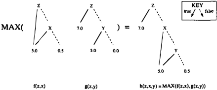
BDDs and ADDs have several useful properties. First, for a given variable ordering, each distinct function has a unique reduced representation. In addition, many common func­ tions can be represented compactly because of isomorphic­ subgraph sharing. Furthermore, efficient algorithms (e.g., depth-first search with a hash table to reuse previously com­ puted results) exist for most common operations, such as addition, multiplication, and maximization. For example, Figure I shows a computation of the maximum of two ADDs. Finally, because BDDs and ADDs have been used

2 We are describing the most common variety of BOD. Numer­ ous variations exist in the literature.

二

extensively in other domains, very efficient implementa­ tions are readily available. As we will see, these properties make ADDs an ideal candidate to represent structured value functions in MDP solution algorithms.

3.2 ADD Representation of MDPs

We assume that the MDP state space is characterized by a set of variables X = {X 1, · · · , X n } . Values of variable X; will be denoted in lowercase (e.g., x;). We assume each X; is boolean, as required by the ADD formalism, though we discuss multi-valued variables in Section 5. Actions are of­ ten most naturally described as having an effect on specific variables under certain conditions, implicitly inducing state transitions. DBN action representations [13, 7] exploit this fact, specifying a local distribution over each variable de­ scribing the (probabilistic)impact an action has on that vari­ able.

A DBN for action a requires two sets of variables, one set X = {X 1, · · · , X n } referring to the state of the system be­ fore action a has been executed, and X' = { x;, · · · , X � } denoting the state after a has been executed. Directed arcs from variables in X to variables in X' indicate direct causal influence and have the usual semantics [17, 13].3 The con­ ditional probability table (CPT) for each post-action vari­ able x; defines a conditional distribution P�. over Xii.e., a's effect on X;-for each instantiatio � of its par­ ents. This can be viewed as a function P� ,( X 1 . . . X n ) . but where the function value (distribution) de p ends only on those Xj that are parents of Xi. No quantification is pro­ vided for pre-action variables X;: since the process is fully observable, we need only use the D BN to predict state tran­ sitions. We require one D BN for each action a E A.

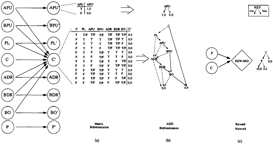
In order to illustrate our representation and algorithm, we introduce a simple adaptation of a process planning prob­ lem taken from [14]. The example involves a factory agent which has the task of connecting two objects A and B. Fig­ ure 2(a) illustrates our representation for the action bolt, where the two parts are bolted together. We see that whether the parts are successfully connected, C, depends on a num­ ber of factors, but is independent of the state of variable P (painted). In contrast, whether part A is punched, APU, after bolting depends only on whether it was punched be­ fore bolting.

Rather than the standard, locally exponential, tabular repre-

3 We ignore the possibility of arcs among post-action variables, disallowing correlations in action effects. See [4) for a treatment of dynamic programming when such correlations exist.

sentation of CPTs, we use ADDs to capture regularities in the CPTs (i.e., to represent the functions P)(,( X1 . . . Xn)). This type of representation exploits contex t -specific inde­ pendence in the distributions [9], and is related to the use of tree representations [7] and rule representations [18] of CPTs in D BNs. Figure 2(b) illustrates the ADD represen­ tation of the CPT for two variables, C' and APU'. While the distribution over C' is a function of its seven parent vari­ ables, this function exhibits considerable regularity, readily apparent by inspection of the table, which is exploited by the ADD. Specifically, the distribution over C' is given by the following formula:

(we ignore the zero entries). Similarly, the ADD for APU' corresponds to:

Reward functions can be represented similarly. Figure 2(c) shows the ADD representation of the reward function for this simple example: the agent is rewarded with 10 if the two objects are connected and painted, with a smaller re­ ward of 5 when the two objects are connected but not painted, and is given no reward when the parts are not con­ nected. The reward function, R(X1, ... ,Xn). is simply

This example action illustrates the type of structure that can be exploited by an ADD representation. Specifically, the CPT for C' clearly exhibits disjunctive structure, where a variety of distinct conditions each give rise to a specific probability of successfully connecting two parts. While this ADD has seven internal nodes and two leaves, a tree repre­ sentation for the same CPT requires 11 internal nodes and 12 leaves. As we will see, this additional structure can be exploited in value iteration. Note also that the standard ma­ trix representation of the CPT requires 128 parameters.

ADDs are often much more compact that trees when rep­ resenting functions, but this is not always the case. The ordering requirement on ADDs means that certain func­ tions can require an exponentially larger ADD representa­ tion than a well-chosen tree; similarly, ADDs can be expo­ nentially smaller than decision trees. Our initial results sug­ gest that such pathological examples are unlikely to arise in most problem domains (see Section 5), and that ADDs offer an advantage over decision trees.

4 Value Iteration using ADDs

In this section, we present an algorithm for optimal pol­ icy construction that avoids the explicit enumeration of the state space. SPUDD (stochastic planning using decision diagrams) implements classical value iteration, but uses ADDs to represent value functions and CPTs. It exploits the regularities in the action and reward networks, made

explicit by the ADD representation described in the previ­ ous section, to discover regularities in the value functions it constructs. This often yields substantial savings in both space and computational time. We first introduce the algo­ rithm in a conceptually clear way, and then describe certain optimizations.

OBDDs have been explored in previous work in AI plan­ ning [11], where universal plans (much like policies) are generated for nondeterministic domains. The motivation in that work, avoiding the combinatorial explosion associated with state space enumeration, is similar to ours; but the de­ tails of the algorithms, and how the representation is used to represent planning domains, is quite different.

4.1 The Basic SPUDD Algorithm

The SPUDD algorithm, shown in Figure 3, implements a form of value iteration, producing a sequence of value functions V0, V 1 , · · ·until the termination condition is met. Each i stage-to-go value function is represented as an ADD denotedVi(X 1 , ... ,Xn). SinceV0 = R,the first value function has an obvious ADD representation. The key in­ sight underlying SPUDD is to exploit the ADD structure of Vi and the MOP representation itself to discover the ap­ propriate ADD structure for Vi+ 1 . Expected value calcula­ tions and maximizations are then performed at each termi­ nal node of the new ADD rather than at each state.

Given an ADD for Vi, Step 3 of SPUDD produces Vi+ 1 . When computing Vi+ 1 , the function Vi is viewed as rep­ resenting values at future states, after a suitable action has been performed with i + 1 stages remaining. So variables in Vi are first replaced by their primed, or post-action, coun­ terparts (Step 3(a)), referring to the state with i stages-to­ go; this prevents them from being confused with unprimed variables that refer to the state with i + 1 stages-to-go. Fig­ ure 4(a) shows the zero stage-to-go primed value diagram, V'0, for our simple example.

For each action a, we then compute an ADD representa­ tion of the function v�+l, denoting the expected value of performing action a with i + 1 stages to go given that V' dictates i stage-to-go value. This requires several steps, described below. First, we note that the ADD-represented functionsP_K,, taken from the action network fora, give the (conditional),probabilities that variables Xi are made true by action a. To fit within the ADD framework, we introduce the negative action diagrams

which gives the probability that a will make Xi false. We then define the dual action diagrams Q'X ; as the ADD rooted at Xi, whose true branch is the action diagram P!X, . and whose false branch is the negative action diagram P!X ; :

Intuitively, Q'X,(x:;xl, ... xn) denotesP(Xi = x:IX 1 = x1, · · ·, Xn = �n) (under action a). Figure 4(a) shows the dual action diagram for the variable C' from the example in Figure 2(b ).

In order to generate V�+ l , we must, for each state s, com­ bine the i stage-to-go value for each state t with the prob­ ability of reaching t from s. We do this by multiplying, in turn, the dual action diagrams for each variable Xj by V'i

-

1. Set V0 = R where R is the immediate reward diagram; set i=O 2. Create dual action diagrams, Q�, (x:, X 1 , ... Xn) for each . a E A, and for each x: E X' 3. RepeatuntiliiV'+1- V ' l l < ·(��13) (a) Swap all variables in X' with primed versions to create X" (b) For all a E A Set temp = V' ' For all primed variables, Xj in V'' temp = temp* Q�, ' 0 Set temp = Sum the sub-diagrams of temp End For over the primed variable Xj Multiply the result by discounting factor {3 and add R to obtain v,; End For (c) Maximize over all v,;·s to create v·+1. (d) Increment i End Repeat
2. Perform one more iteration and assign to each terminal node the actions a which contributed the value in the value ADD at that node; this yields the !-optimal policy ADD, 1r · . Note that terminal nodes which have the same values for multiple actions are assigned all possible actions in 1r · .
3. Return the value diagram v·+! and the optimal policy 1r·.

Figure 3: SPUDD algorithm

and then eliminating Xj by summing over its values in the resultant ADD. More precisely, by multiplyingQi, by V'i, ' we obtain a function f(Xf, ···,X�, X 1 , · · ·Xn) where

(assuming transitions induced by action a). This intermedi­ ate calculation is illustrated in Figure 4(b ), where the dual diagram for variable C' is the first to be multiplied by V'0· Note that C' lies at the root of this ADD. Once this func­ tion f is obtained, we can eliminate dependence of future value on the specific value of Xj by taking an expectation over both of its truth values. Th1s is done by summing the left and right subgraphs of the ADD for f, leaving us with the function

This is illustrated in Figure 4(c), where the variable C' is eliminated. This ADD denotes the expected fUture value (or 0 stage-to-go value) as a function of the parents of C' with

1 stage-to-go and all post-action variables except C' with 0 stages-to-go.

This process is repeated for each post-action variable Xj that occurs in the ADD for V'i: we first multiply Qi, into ' the intermediate value ADD, then eliminate that variable by taking an expectation over its values. Once all primed vari­ ables have been eliminated, we are left with a function

By the independence assumptions embodied in the action network, this is precisely the expected future value of per­ forming action a. By adding the reward ADD R to this function, we obtain an ADD representation of v;+1. Fig­ ure 5 shows the result for our simple example. The remain­ ing primed variable P' in Figure 4(c) has been removed, producing V�olt using a discount factor of 0.9. Finally, we take the maximum over all actions to produce the Vi+1 dia­ gram. Given ADDs for each vj+1, this requires simply that one construct the ADD representing maXaeA vj+1 .

The stopping criterion in Equation 3 is implemented by comparing each pair of successive ADDs, V'+1 and V'. Once the value function has converged, the £-optimal pol­ icy, or policy ADD, is extracted by performing one further dynamic programming backup, and assigning to each ter­ minal node the actions which produced the maximimizing value. Since each terminal node represents some state set of states S, the set of actions thus determined are each optimal for any s E S.

4.2 Optimizations

The algorithm as described in the last section, and as shown in Figure 3, suffers from certain practical difficulties which make it necessary to introduce various optimizations in or­ der to improve efficiency with respect to both space and time. The problems arise in Step 3(b) when V'i is multi­ plied by the dual action diagrams Q·. Since there are po­ tentially n primed variables in the ADD for V'i and n un­ primed variables in the ADD for Q·, there is an interme­ diate step in which a diagram is created with (potentially) up to 2n variables. Although this will not be the case in general, it was deemed necessary to modify the method in order to deal with the possibility of this problem arising. Furthermore, a large computational overhead is introduced by re-calculating the joint probability distributions over the primed variables at each iteration. In this section, we first discuss optimizations for dealing with space, followed by a method for optimizing computation time.

The increase in the diagram size during Step 3(b) of the al­ gorithm can be countered by approaching the multiplica­ tions and sums slightly differently. Instead of blindly mul­ tiplying the V" �Y the dual action diagram for the variable at the root of V", we can traverse the ADD for V" to the level of the last variable in the ADD ordering, then mul­ tiply and sum the sub-diagrams rooted at this variable by

the corresponding dual diagram. This process will only re­ move the dependency of the V'; on a primed variable for a given branch, and will therefore only introduce a single diagram of n unprimed variables at a leaf node of V';. By recursively carrying out this procedure using the structure of the ADD for V';, the intermediate stages never grow too large. Essentially, the additional unprimed variables are in­ troduced only at specific points in the ADD and the corre­ sponding primed variable immediately eliminated-this is much like the tree-structured dynamic programming algo­ rithm of [7].

Unfortunately, this method requires a great deal of unnec­ essary, repeated computation. Since the action diagrams for a given problem do not change during the generation of a policy, the joint probability distribution Pr(s, a, t) from Equation 2 could be_ pre-computed. In our case, this means we could take the product of all dual action diagrams for a given action a, as shown in Equation 5 below, prior to a spe­ cific value iteration. We refer to this product diagram, p·, as the complete action diagram for action a:

The resulting function p· provides a representation of the state transition probabilities for action a. This explicit p· function could then be multiplied by the V'" during Step 3 of the algorithm, and then primed variables eliminated. Although this may lead to a substantial savings in compu­ tation time, it will again generate diagrams with up to 2n variables.

As a compromise, we implemented a method where the space-time trade-off can be addressed explicitly. A "tun­ ing knob" enables the user to find a middle ground between the two methods mentioned above. We accomplish this by pre-computing only subsets of the complete action di­ agram. That is, we break the large diagram up into a few smaller pieces. The set of variables (X1, .. . , Xn) is di­ vided into m subsets, preserving the total ordering (e.g. , [X1, ... ,X;,], [X;,+l, .. . ,X;2], ... , [X;m, ... Xn]). and the complete action diagrams are pre-computed for each subset (e. g., (P"(Xi,, . . . 'x:i+l , VJ' . . . 'Xn)). Step 3(b) of the algorithm must be modified as shown in Figure 6. The primed value diagram V'; is traversed to the top of the second level (i 1 + 1 ), and the procedure is carried out re­ cursively on each sub-diagram rooted at variables Xj,+1. If a level is reached with no variables below it, then the sub­ diagram rooted at each variable Xjm of VI i is multiplied

二

I. Set BIG ADD = user-specified limit for size of graphs Set temp = ADD constant I Set k = 1; m = 0 size = 0 2. While k < number of variables j=k i, = k While size < BIGADD Set temp = temp · Q�, size = no. of internal n � des in temp k=k+1 End While P0(vj, ... , v�_1, V I , ... , Vn) =temp m=m+l End While 3. Repeatunti!IIV;+ I - V ; ll < '';il (c) For a l i a E A Set lastlevel = m CaD pRew{V"' ,Pa , 0 , 1)

procedure pRew (value,action,var ,nexLlevel) If var > inextJevel If var > iza�tJevel result = value lastlevel = lastlevel - 1 Else else temp= pRew (value,action,var,nexLlevel + 1) temp = temp · act result = sum all sub-diagrams of temp over primed variables, vj j > iza,tJevel tempT= prRew(then(value), action,level + 1,nextJevel) tempE= prRew(else(value), action,level + 1,nextJevel) result =tree rooted at v :levet with then, else branches: tempT,tempE, resp. return result

with the corresponding subset of the complete action dia­ gram, P4(XL, .. . ,X�,X1, . . . , X n ). and summed over primed variables X£, k > im. In this way, the diagrams are kept small by making sure that enough elimination oc­ curs to balance the effects of multiplying by complete ac­ tion diagrams. The space and time requirements can then be controlled by the number of subsets the complete action diagrams are broken into. In theory, the more subsets, the smaller the space requirements and the larger the time re­ quirements. Although we have been able to produce sub­ stantial changes in the space and time requirements of the algorithm using this tuning knob, its effects are still un­ clear. At present, we choose the m subsets of variables by simply building the complete action diagrams according to some variable ordering until they reach a user-defined size limit, at which point we start on the next subset. We note that this space-time tradeoff bears some resemblance to the space-time tradeoffs that arise in probabilistic inference al­ gorithms like variable elimination [15].

Although we have not implemented heuristics for variable ordering, there are some simple ordering methods that could improve space efficiency. For instance, if we order vari­ ables so that primed variables with many shared parents are eliminated together, the number of unprimed variables in­ troduced will be kept relatively small relative to the number of primed variables eliminated. More importantly, we must develop more refined heuristics that keep the ADDs small rather than minimizing the number of variables introduced.

This revised procedure (Figure 6) has a small inefficiency, as our results in the next section will show. Since we are pre-computing subsets of the complete action diagrams, any variables which are included in the domain, but are not rel­ evant to its solution, will be included in these pre-computed diagrams. This will increase the size of the intermediate representations and will add overhead in computation time. It is important to be able to discard them, and to only com­ pute the policy over variables that are relevant to the value function and policy [7]. A possible way to deal with these types of variables in our algorithm would be to progres­ sively build the complete action diagrams during the iter­ ative procedure. In this way, only the variables relevant to the domain would be added.

5 Data and Results

The procedure described above was implemented using the CUDD package [20], a library of C routines which pro­ vides support for manipulation of ADDs. Experimental re­ sults described in this section were all obtained using a dual­ processor SUN SPARC Ultra 60 running at 300Mhz with I Gb of RAM , with only a single processor being used. The SPUDD algorithm was tested on three different types of examples, each type having MDP instances with different numbers of variables, hence a wide variety of state space sizes. The first example class consists of various adapta­ tions of a process planning problem taken from [14]. The second and third example classes consist of synthetic prob­ lems taken from [7, 8]. These are designed to test best- and worst-case behavior of SPUDD.4

The first example class consists of process planning prob­ lems taken from [ 1 4], involving a factory agent which must paint two objects and connect them. The objects must be smoothed, shaped and polished and possibly drilled before painting, each of which actions require a number of tools which are possibly available. Various painting and connec­ tion methods are represented, each having an effect on the quality of the job, and each requiring tools. The final prod­ uct is rewarded according to what kind of quality is needed. Rewards range from 0 to 10 and a discounting factor of 0. 9 was used throughout.

The examples used here, unlike the one described in Sec­ tion 3, were not designed with any structure in mind which could be taken advantage of by an ADD representation. In the original problem specification, three ternary variables were used to represent painting quality of each object (good, poor or false), and the connection quality (good, bad or false). However, as discussed above, ADDs can only rep-

4 Data for these problems can be found at the Web page: www.cs.ubc.ca/spider/staubin/Spudd/index.htrnl.

resent binary variables, so that each ternary variable was expanded into two binary ones. For example, the vari­ able connected, describing the type of connection between the two objects, was represented by boolean variables con­ nected and connected.well. This expansion enlarges the state space by a factor of 4/3 for each ternary variable so expanded (by introducing unreachable states). A number of FACTORY examples were devised, with state space sizes ranging from 55 thousand to 268 million.

Optimal policies were generated using SPUDD and a struc­ tured policy iteration (SPI) implementation for comparison purposes [7). Results, displayed in Table I, are presented for SPUDD running on six FACTORY examples, and for SPI running on five. SPI was not run on the factory4 ex­ ample, because its estimated time and space requirements exceeded available capacity. SPI implements modified pol­ icy iteration using trees to represent CPTs and intermedi­ ate value and policy functions. SPI, however, does allow multi-valued variables-so versions of each example were tested in SPI using both ternary variables, and thier binary expansion. Table I shows the number of ternary variables in each example, along with the total number of variables. The state space sizes of each FACTORY example are shown for both the original and the binary-expansion formulations. SPUDD was only run on the binary-expanded versions.

The examples labelled factory/ andfactory2 differ only by a single binary variable, which is not affected by any action in the domain, and which does not itself affect any other variables. Hence, the number of internal nodes resulting in Table I are identical for the two examples. This vari­ able was added in order to show how structured represen­ tations like SPUDD and SPI can effectively discard vari­ ables which do not affect the problem at hand, as discussed in Section 4.2. Since SPUDD pre-computes the complete action diagrams, as shown in Figure 6, the running time for SPUDD almost doubles when this new variable is added, since it creates overhead for the iterative procedure. This problem could be circumvented using the method described at the end of Section 4.2.

Running times are shown for SPUDD and SPI. However, the algorithms do not lend themselves easily to comparisons of running times, since implementation details cloud the re­ sults; so running times will not be discussed further here. The SPI results are shown in order to compare the sizes of the final value function representations, which give an indication of complexity for policy generation algorithms. However, a question arises when comparing such numbers about the variable orderings, as mentioned in Section 3. The variable ordering for SPUDD is chosen prior to runtime and remains the same during the entire process. No special tech­ niques were used to choose the ordering, although it may be argued that good orderings could be gleaned from the MDP specification. Variable orderings within the branches of the tree structure in the SPI algorithm are determined primarily by the choice of ordering in the reward function and action descriptions [7]. Again, no special techniques were used to choose the variable ordering in SPI. Finding the optimal variable orderings in either case is a difficult problem, and we assume here that neither algorithm has an advantage in this regard. Dynamic reordering algorithms are available in

CUDD, and have been implemented but not yet fully tested in SPUDD (see below).

In order to compare representation sizes, we compare the number of internal nodes in the value function represen­ tations only. This is most important when doing dynamic programming back-up steps and is a large factor in deter­ mining both running time and space requirements. Further­ more, we compare numbers from SPUDD using binary rep­ resentations with numbers from SPI using binary/ternary representations in order not to disadvantage SPI, which can make use of ternary variables. We also compare both imple­ mentations using only binary variables. The equivalent tree leaves column in Table I gives the number of leaves of the totally ordered binary tree (and hence the number of inter­ nal nodes) that results in expanding the value ADD gener­ ated by SPUDD. These numbers give the size of a tree that would be generated if a total ordering was imposed. Com­ paring these numbers with the numbers generated by SPI give an indication of the savings that occur due to the re­ laxation of the total ordering constraint. The rightmost col­ umn in Table I shows the ratio of the number of internal nodes in the tree representation to the number in the ADD representation. We see that reductions of up to 30 times are possible, when comparing only binary representations to binary/ternary representations, and reductions of over 40 times when comparing the same binary representations. These space savings also showed up in the amount of mem­ ory used. For example, thefactory3 example took 691Mb of memory using SPI, and only 148Mb using SPUDD. The factory4 example took 378Mb of space using SPUDD.

The BIGADD limit (see Figure 6) was set to 10000 for the factory, factoryO, factory/ and factory2 examples and to 20000 in the factory] and factory4 examples. These lim­ its broke up the complete action diagrams into m == 2 or 3 pieces, with typically 6000-10000 nodes in the first and second and under I 000 nodes in the third if it existed. In the large examples (factory2, 3 and 4), it was not possible (with 1Gb of RAM) to generate the full complete action diagram (m == 1), and running times became too large when BI­ GADD was set to 1. The functionality of this ''tuning knob" was not fully investigated, but, along with studies of differ­ ent heuristics for variable grouping, is an interesting avenue for future exploration.

For comparison purposes, fiat (unstructured) value iteration was run on both the factory and factoryO examples. The times taken for these problems were 895 and 4579 seconds, respectively. For the larger problems, memory limitations precluded completion of the flat algorithm.

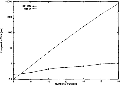
In order to examine the worst-case behaviour, we tested SPUDD on a series of examples, drawn from [7, 8], in which every state has a unique value; hence, the ADD rep­ resenting the value function will have a number of termi­ nal nodes exponential in the number of state variables. The problem EXPON involves n ordered propositions and n actions, one for each proposition. Each action makes its corresponding proposition true, but causes all propositions lower in the order to become false. A reward is given only if all variables are true. The problem is representable in O(n2) space using ADDs; but the optimal policy winds through the entire state space like a binary counter. This

Table 1: Results for FACTORY examples.

Example Name	State space size			SPUDD - Value				SPI· Value			internal	ratio of
	variables tematy	lOla]	states	time (s)	internal nodes	leaves	equiv. tree leaves	time (s)	nodes	leaves	tree nodes: ADD nodes
factory	3 0	14 17	55296 131072	- 78.0	828	147	8937	2210.6 2188.23	6721 7879 9513 9514		8.12 11.48
factoryO	3 0	16 19	221184 524288	- 111.4	1137	147	14888	5763.1 6238.4	15794 i2611	18451 22612	13.89 19.89
factory I	3 0	18 21	884736 2097132	279.0	2169	178	49558	14731.9 15430.6	31676 44304	37315 44305	14.60 20.43
factory2	3 0	19 22	1769472 4194304	462.1	- 2169	178	49558	14742.4 15465.0	31676 44304	37315 44305	14.60 20.43
factory3	4 0	21 25	10616832 33554432	3609.4	- 4711	208	242840	98340.0 112760.1	138056 193318	168207 193319	29.31 41.04
factory4	4 0	24 28	63700992 268435456	14651.5	- 7431	238	707890		- -		- -

problem causes worst-case behaviour for SPUDD because all 2 n states have different values. SPUDD was tested on the EXPON example with 6, 8, 10 and 12 variables, leading to state spaces with sizes 64, 256, 1024 and 4096, respec­ tively. The initial reward and the discounting factor in these examples must be scaled to accommodate the 2n -step look­ ahead for the largest problem (12 variables), and were set to 1016 and 0.99, respectively.5 Figure 7 compares the run­ ning times of SPUDD and (flat) value iteration plotted (in log scale) as a function of the number of variables. Run­ ning times for both algorithms exhibit exponential growth with the number of variables, as expected. 6 It is not sur­ prising that flat value iteration performs better in this type of problem since there is absolutely no structure that can be exploited by SPUD D. However, the overhead involved with creating ADDs is not overly severe, and tends to diminish as the problems grow larger. With n = 12, SPUDD takes less than 10 times longer than value iteration.

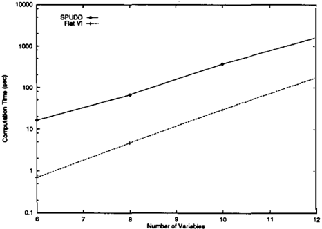
One can similarly construct a "best-case" series of exam­ ples, where the value function grows linearly in the number of problem variables. Specifically, the problem LINEAR involves n variables and has n+ 1 distinct values. The MDP can be represented in 0 ( n 2) space using ADDs and the op­ timal value function can be represented in 0( n) space with an ADD (see [8] for further details)? Hence, the inherent structure of such a problem can easily be exploited. As seen in Figure 8, SPUDD clearly takes advantage of the struc­ ture in the problem, as its running time increases linearly with the number of variables, compared to an exponential

5 Since the value obtained at the state furthest from the goal is the goal reward discounted by the number of system states (since each must be visited along the way), the goal reward must be set very high to ensure that the value at this state is not (practically) zero.

6The running times are especially large due to the nature of the problem which requires a large number of iterations of alue itera­ tion to converge.

7 Of course, best- case behavior for SPUDD involves a problem in which all variables are irrelevant to the value function. This problem represents a "best case" in which all variables are re­ quired in the prediction of state value.

increase in running time associated with flat value iteration.

6 Concluding Remarks

In this paper, we described SPUDD, an implementation of value iteration, for solving MDPs using ADDs. The ADD representation captures some regularities in system dynam­ ics, reward and value, thus yielding a simple and efficient representation of the planning problem. By using such a compact representation, we are able to solve certain types of problems that cannot be dealt with using current tech­ niques, including explicit matrix and decision tree methods. Though the technique described in this paper has not yet been tested extensively on realistic domains, our prelimi­ nary results are encouraging.

One drawback of using ADDs is the requirement that vari­ ables be boolean. Any (finite-valued) non-boolean vari­ able can be split into a number of boolean variables, gen­ erally in a way that preserves at least some of the struc­ ture of the original problem (see above), though it often

1 0000.-----�--�--,--r---,

makes the new state space larger than the original. Con­ ceptually, there is no difficulty in allowing ADDs to deal with multi-valued variables (all algorithms and canonicity results carry over easily). However, for domains with rela­ tively few multi-valued variables, SPUDD does not appear to be handicapped by the requirement of variable splitting.

At present, SPUDD uses a static user-defined variable or­ dering in order not to cloud the initial results with the ef­ fects of dynamic variable reordering. However, dynamic reordering of the variables at runtime can make significant improvements in both the space required, by finding a more compact representation, and in the running time, by choos­ ing more appropriate subsets of variables as discussed in Section 4.2. The CUDD package provides a rich set of dynamic reordering algorithms [20]. Typically, when the ADD grows too large, variable reorderings are attempted by following one of these algorithms, and a new ordering is chosen which minimizes the space needed. Some of the available techniques are slight variations of existing tech­ niques while some others were specifically developed for the package. It may be necessary, however, to implement a new heuristic which takes into account the variable subsets which influence the running time. Future work will include more complete experimentation with automatic dynamic reordering in SPUDD. Another extension of SPUDD would be the implementation of other dynamic programming algo­ rithms, such as modified policy iteration, which are gener­ ally considered to converge more quickly than value itera­ tion in practice. Finally, we hope to explore approximation methods within the ADD framework, such as have previ­ ously been researched in the context of decision trees [6].

Acknowledgements

Thanks to Richard Dearden for helpful comments and for providing both his SPI code and example descriptions for comparison purposes. St-Aubin was supported by NSERC. Hu was supported by NSERC. Boutilier was supported by NSERC Research Grant OGP0121843 and IRIS-III Project "Dealing with Actions."

References

• [I] R. Iris Bahar, E. A. Frohm, C. M. Gaona, G. D. Hachtel, E. Macii, A. Pardo, and F. Somenzi. Algebraic decision dia­ grams and their applications. Inti. Conf Computer - Aided Design, 188-191,1EEE, 1993.
• (2] R. E. Bellman. Dynamic Programming. Princeton Univer­ sity Press, Princeton, 1957.
• D.P. Bertsekas and D. A. Castanon. Adaptive aggregation for infinite horizon dynamic programming. IEEE Trans. Aut. Cont., 34:589-598, 1989.
• C. Boutilier. Correlated action effects in decision theoretic regression. Proc. UAI-97, pp.30-37, Providence, RI, 1997.
• C. Boutilier, T. Dean, and S. Hanks. Decision theoretic plan­ ning: Structural assumptions and computational leverage. J. Artif. Intel. Research, 1999. To appear.
• C. Boutilier and R. Dearden. Approximating value trees in structured dynamic programming. Proc. Inti. Conf Machine Learning, pp.54--62, Bari, Italy, 1996.
• C. Boutilier, R. Dearden, and M. Goldszmidt. Exploiting structure in policy construction. Proc. IJCAI-95, pp.II04l l l l , Montreal, 1995.
• C. Boutilier, R. Dearden, and M. Goldszmidt. Stochas­ tic dynamic programming with factored representations. manuscript, 1999.
• C. Boutilier, N. Friedman, M. Goldszmidt, and D. Koller. Context-specific independence in Bayesian networks. Proc. UAJ-96, pp.li5-123,Portland, OR,i996.
• R. E. Bryant. Graph-based algorithms for boolean function manipulation. IEEE Trans. Comp., C-35(8):677-691, 1986.
• A. Cimatti, M. Roveri, and P. Traverso. Automatic obdd­ based generation of universal plans in non-deterministic do­ mains. Proc. AAAJ-98, pp.875-881, 1998.
• [ 12] T. Dean and R. Givan. Model minimization in Markov de­ cision processes. Proc. AAAI-97, pp.l 06--111, Providence, 1997.
• T. Dean and K. Kanazawa. A modelfor reasoningabout per­ sistence and causation. Comp. Intel., 5(3): 142-150, 1989.
• R. Dearden and C. Boutilier. Abstraction and approximate decision theoretic planning. Artif. Intel., 89:219-283, 1997.
• [ 15] R. Dechter. Topological parameters for time-space tradeoff. Proc. UA!- 96, pp.220-227, Portland, OR, 1996.
• S. Hanks and D. V. McDermott. Modelinga dynamicandun­ certain world i: Symbolic and probabilistic reasoning about change. Artif. InteL, J 994.
• [ 17] J. Pearl. Probabilistic Reasoning in Intelligent Systems: Net­ works of Plausible Inference. Morgan Kaufmann, San Ma­ teo, 1988.
• [ 18] D. Poole. Exploiting the rule structure for decision making within the independent choice logic. Proc. UA!-95, pp.454463, Montreal, 1995.
• M. L. Puterman. Markov Decision Processes: Discrete Stochastic Dynamic Programming. Wiley, New York, NY., 1994.
• F. Somenzi. CUDD: CU decision diagram package. Avail­ able from ftp: I /vlsi .colorado. edu/pub/, 1998.