Sufficiency, Separability and Temporal Probabilistic Models Avi Pfeffer Abstract 1 Introduction 2 Sufficiency and Separability 2.1 Comparison to Other Structures 2.2 Exploiting Separability in Bayesian Network Inference 3 Conditional Separability 4 Separability in Temporal Models 4.1 Self-Sufficiency 4.2 Identifying Self-Sufficient Families 4.3 Hierarchical Decomposition 4.4 Observations 5 Conclusions and Speculations References

1301.2301

Sufficiency, Separability and Temporal Probabilistic Models

Avi Pfeffer

Division of Engineering and Applied Sciences Harvard University [email protected]

Abstract

Suppose we are given the conditional proba bility of one variable given some other vari ables. Normally the full joint distribution over the conditioning variables is required to determine the probability of the conditioned variable. Under what circumstances are the marginal distributions over the conditioning variables sufficient to determine the probabil ity of the conditioned variable? Sufficiency in this sense is equivalent to additive separa bility of the conditional probability distribu tion. Such separability structure is natural and can be exploited for efficient inference. Separability has a natural generalization to conditional separability.

Separability provides a precise notion of hi erarchical decomposition in temporal prob abilistic models. Given a system that is decomposed into separable subsystems, ex act marginal probabilities over subsystems at future points in time can be computed by propagating marginal subsystem probabil ities, rather t han complete system joint prob abilities. Thus, separability can make exact prediction tractable. However, observations can break separability, so exact monitoring of dynamic systems remains hard.

1 Introduction

Bayesian networks (BNs) use conditional indepen dence in order to provide compact representations of probability distributions. This structure also supports efficient inference algorithms. Dynamic Bayesian net works (DBNs) use a similar conditional independence structure in the representation of temporal probabilis tic models. However, this structure has proven resis tant to exploitation for efficient inference. The prob- lem, of course, is that even when there is local condi tional independence in the dynamic model, in the long run all variables become correlated. It would seem therefore, that if we want to perform exact inference, we can do no better than to compute a complete joint probability distribution over the set of state variables at time t (or at least the subset of the state variables that have an effect on the next state).

There is a strong intuition that many dynamic systems can be hierarchically decomposed into weakly inter acting subsystems, and such a decomposition should be capable of supporting efficient reasoning about the system. However, previous attempts to repre sent such decompositions (e.g. [FKP98 ] ) have run into the same inference difficulties as DBNs. Boyen and Koller [BK98, BK99] have shown that hierarchical structure can be exploited for approximate monitor ing, but this only applies to approximate inference, and the quality of the approximation is highly sensitive to the numbers in the conditional probability tables and not just the structure. The search for inference supporting structures in dynamic systems is still on.

This paper identifies such a structure. The key idea is that even if all the state variables become correlated, it may not be necessary to actually compute complete joint distributions over the state. If we are only inter ested in marginal probabilities of particular variables, can we reason by propagating marginal distributions over subsets of state variables rather than complete joint distributions? What structure would support that? The approach is similar in spirit to Lauritzen's method [Lau92] for inference with conditional Gaus sian models. Even though the posterior marginals are not Gaussian, their means and variances can be prop agated exactly as if they were.

In studying this question about dynamic systems, I was led to a more specific question about static BNs. Suppose a variable Y has parents X1, . .. , Xn. Under what circumstances are the xi sufficient for P(Y I X1 , . . . , Xn), in the sense that it is sufficient to know

the marginals over the Xi in order to determine P(Y), rather than the full joint over the Xi? It turns out that sufficiency is equivalent to additive separability of the conditional probability P(Y I XI, . . . , Xn) into terms that depend on each of the Xi individually. Separa bility is a natural structure, and is closely related to a form of context-specific ind e p e n den c e [BFGK96]. It is quite easy to exploit separability for efficient infer ence. There is also a natural generalization to a more complex notion of conditional separability.

While sufficiency and separability are useful in their own right for static ENs, what about the original ques tion about temporal models? Can we find subsets of state variables that are self-sufficient, i.e., that the marginals over these variables at time t are sufficient to obtain correct marginals over them at time t + 1? It turns out that some temporal systems can indeed be hierarchically decomposed into subsystems in a way that corresponds to separability. As a result, it is indeed possible to predict the marginal distributions over the state of a subsystem by propagating marginal probabilities of the different subsystems.

This is a satisfying result, since it provides a tractable exact solution of one problem in temporal probabilis tic inference. However, this is only a limited success, because as soon as observations are introduced, prop agating marginals is no longer correct, and therefore the exact monitoring problem is still hard, even for systems that decompose into separable subsystems.

2 Sufficiency and Separability

Let us begin with a simple situation. Consider three variables X, Y, and Z, with Z depending on X andY according to the conditional probability distribution P(Z 1 XY). I will use the notation AXY to denote the space of probability distributions over XY, and for q E Ll XY, qx denotes the marginal of q over X.

If a joint distribution q over XY is given, P(Z) is determined by L:zy q(xy)P(Z I xy). Thus the condi tional probability of Z given XY determines a function from A,X Y to Az. Normally, this function depends on the joint distribution q over XY, but in some cases it is fully determined by the rnarginals qx and qy. This idea leads to the following definition.

Definition 2.1: Let X, Y and Z be variables, and let P(Z I XY) be given. Define the function �P : A,X Y -+ t:J.Z by �P(q) = L:zy q(xy)P (Z 1 xy). We say that X and Y are sufficient for Z under P if, for any q 1 , q2 in f:J.XY such that ql = qJc and q� = q}, � P (q l ) = cp P ( q 2 ). W h en P is clear from <:ontext, we will simply write .P and drop "under P". I

Sufficiency is a desirable inference property. Suppose we have a BN containing X, Y and Z as well as other nodes, and we want to compute P(Z) given some ev idence e. Suppose that X and Y are the parents of Z, an d d-separate Z from e, but are not themselves conditionally independent given e. One way to com pute P(Z) is to compute P(XY I e) and then apply .P. However, if X and Y are sufficient for Z, we can com pute P(X I e) and P(Y I e) separately, and apply .Pas if X andY were independent given e. Is there a rep resentational structure corresponding to this inference property? It turns out that sufficiency is equivalent to additive separability of the conditional probability distribution, defined as follows:

Definition 2.2: P(Z I X Y ) is separable if there exist conditional distributions Px(Z I X) and Py(Z I Y), and-y E [0, 1], such that P(Z I X Y) = rPx(Z I X)+ (1 -{)Py(Z I Y). I

Theorem 2.3: X andY are sufficient for Z iff P(Z I XY) is separable.

Proof: "If" is easy. If P(Z I XY) is separable,

.P(q) = Lzv q(xy)P(Z I xy)

= I'Lz(L:11 q( xy ))P x (Z I x)+ (1-1) :l:11 ( Ez q(xy))Py(Z I y)

= L:z11 q(xy)[{Px (Z I x) + ( 1 -r)Py(Z I y)]

= 7 L:z qx(x)Px(Z I x ) + (17) L:11 qy(y)Py(Z I y).

so �(q) depends only on the marginals qx and qy.

For "only if", assume X and Y are sufficient for Z, and let Zl be argmaxz(maxz11 P(z I xy) - minz11 P(z I xy)). I.e., z1 is the value of Z most affected by XY. Let Xt,Yl be argminzyP(zl I xy), and let Pt = P(Z I X1Y1). Write a1 = P(Z I XiYt)- P1, and f3; ::: P(Z I XIY;)- P1. Now, for any i and j, consider the distributions q1 and q2 where q1 assigns probabil ity 1/4 to each of the assignments (xl!YI), (Xt,Yj), (x.,yi), and (x1,yj), while q2 assigns probability 1/2 to each of (x1, yl) and ( xi, Yi ). Since q 1 and q2 have the same marginals, by sufficiency �(q1) = .P(q2), so P(Z I XlYl)+P(Z I XiYj) = P(Z I XlYj)+P(Z I XiYI), and therefore P(Z I X i Y; ) = H + ai + f3;.

Write a · =max; P(z1 I x;y1)-P(z1 I X I Y l) and {3* = max; P(zt I XtY;)- P(z1 I x1yt), and set I= a·a;.f3 . . Set P x(x i ) = P1 + *ai, and Py(y;) = P1 + 1�7f3;· Then P(Z I X;Yi) = ')' Px(Z I xi)+ (1-'Y)Py(Z \ Yi), as required. It is not hard to show that Px (Z I xi) and Py(Z I Y;) are probability distributions- details are omitted. I

Separability has a simple intuitive interpretation. The dependent variable Z is only influenced by one of its

parents X or Y, but we don't know which. We can imagine a latent variable that determines which of X and Y actually influences Z. With probability 1 the actual parent is X, and with probability 1-1 it is Y.

If a* + j3* < 1 (in the notation of the proof), the separation of P(Z I XY) is not unique. The remaining probability mass 1 -a* -j3* can be divided in any way between P x and Py. The choice of 1 == 0,o;_13· is particularly natural. a* is the maximum possible effect X can have on Z if Y is held fixed, while {3* is the maximum effect of Y as X is held fixed, so together a* and {3* can be viewed as determining the relative importance of the two parents.

The a b ov e definitions and analysis can be generalized to the case where Z has multiple parents X1, ... , Xn. cJ> is now a function from .6. x 1, ... ,Xn to .6.z given by cJ> ( q ) = L:.,1, ··· ,xn q(xl, . . . ,xn)P(Z I X1, . · · ,xn)· We say that X 1, . · . , X n are sufficient for Z if cJ> ( q) de pends only on the marginals of q over the individual x,. We say that P(Z I x l ' ... , Xn) is separable if it can be written as E, I;P;(Z I X;), where the P, are conditional distributions and I:; li = 1. Using induc tion, and similar ideas to the proof of Theorem 2.3, one can show that X 1, ... , X n are sufficient for Z iff P(Z I X 1 , ... ,Xn) is separable.

2.1 Comparison to Other Structures

Separability is incomparable to conditional indepen dence. X and Y may be conditionally independent given Z, but not sufficient for Z, and vice versa. How ever, if Y is conditionally independent from Z given X, then trivially X and Y are sufficient for Z.

Separability is closely related to context-specific inde pendence (CSI) [BFGK96]. In fact, it can be viewed as a case of CSI where the context variable is latent. Sep arability corresponds to a strong form of CSI, where only one parent is relevant given the context.

Another framework which superficially has some of the same properties as separability is that of causal inde pendence (HB94], which includes the well-known noisy or model. In this framework, one also gets a decompi sition of a large conditional probability distribution in terms of individual dependence on each of the parents. However, separability and causal independence are not related; they correspond to two very different ways in which causes can interact. With causal independence, the different causes are all active simultaneously, but their actions happen independently. With separabil ity, exactly one of the different causes is active, but we don't know which. Causally independent models do not have the sufficiency property.

Separability is related to the concept of synergy from the qualitative probabilistic network (QPN) frame work [Wel90]. Additive synergy characterizes whether the different causes of an effect reinforce each other or interfere with each other. Separable conditional dis tributions exhibit zero synergy - the different causes neither reinforce nor interfere with each other, because only one of them is actually active. In contrast, the noisy-or model exhibits negative synergy; if multiple causes are on, some of their work is wasted because another cause would have achieved the effect anyway.

2.2 Exploiting Separability in Bayesian Network Inference

Earlier I described how sufficiency can be used to sim plify particular BN computations. It is in fact possible to exploit separability in a general way in BN infer ence. One idea is to make the latent selection vari able explicit, and then use methods that have been proposed for exploiting CSI. Two methods are pro posed in [BFGK96]. One is to condition on the con text variable, with the resulting networks being much simpler. This method is hard to integrate into most BN implementations, which do not use conditioning. The second method is based on a network transfor mation, which introduces explicit multiplexer nodes to represent models with CSI. In some cases, this can produce a simpler network than the original. How ever, this transformation is of no benefit in our case, since the selector variable is essentially already acting as a multiplexer; the result node after the transforma tion will have as many parents as before. Poole and Zhang [Poo97, ZP99] provide a comprehensive method for exploiting CSI in inference, based on an extended version of the variable elimination algorithm that uses either partial functions or rules. While this method could be used for separability, it requires a significant extension to standard BN inference methods.

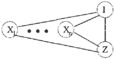
Figure 1: Graph resulting from separability decompo sition

As it happens, there is a simple way to exploit separa bility within the standard variable elimination or junc tion tree inference frameworks. If P(Z I xl, ... ,Xn) is separable, it has the form Ei liPi(Z I Xi)· The idea is to turn this summation into a sum-of-products expression, that can then be used in variable elimina tion. This is achieved by making the selection vari able I explicit, and introducing a factor 9i(I, Z, X;)

fori = 1, . . . , n, where

Formula not decoded

Now,

.Ed1j9;(i,z,x;) = L:;g;(i,z,xi)IJ # ig;(i,Z,Xj) = E;'Y;P;(z I x,) = P;(z I Xt, · . . ,xn ) · We can therefore replace P(Z j X1, .. . ,Xn) with the sum-of-products expression Ei nj 9;(1, z, Xj)· The benefits of this transformation should be clear from looking at the graph corresponding to this expression, shown in Fig ure 1. The graph is triangulated, and contains n cliques of size 3, as opposed to the clique of size n for P(Z I xl, .. . 'Xn)·

This decomposition took advantage of the fact that separability corresponds to a special form of csr in which there is a single context variable that is used to determine which parent is relevant. In conjunction with the transformation from [BFGK96], it can actu ally be used as a general method for dealing with CSI within a standard inference algorithm. The transfor mation shows how to transform any tree-structured conditional probability table into a network with mul tiplexers. The transformation presented here can then be used to replace the multiplexer CPTs with sum-of products expressions.

3 Conditional Separability

Definitions 2.1 and 2.2 generalize naturally to cases where X and Y are sets of variables. If they are dis joint, Theorem 2.3 continues to hold of course, because X and Y can be treated as individual variables taking values in the product space. However, if they are not disjoint, Theorem 2.3 fails. It is possible for X and Y to be sufficient for Z, while P(Z l XU Y) is not expressiblea.·qPx(Z I X)+(1-'Y)Py(Z I Y). For ex ample, suppose X, W ,Y and Z are Boolean variables, and suppose P(z I XWY) is 1 if (x!\w)V(y!\w) holds, 0 otherwise. Then <P(q) = Exw v q(xwy)P(Z I xwy) = Qxw(x !\ w) + qwy(y !\ w) and therefore {X, W} and {W, Y} are sufficient for Z. However, it can easily be checked that P(Z I XWY) cannot be w r i tt e n as 'YPxw(Z I XW) + (1"f ) P w y ( Z I WY). In order to restore a version of Theorem 2.3, we need to intro duce the notion of conditional separability. Notation: if W �X, U =X- W, and we are given P(Z I X) and a value w of W, pw(z I U) is the conditional distribution defined by pw(z I u) = P(z I uw).

Definition 3.1: Let X and Y be sets of variables, let Z ¢ X U Y be a variable, and let W r;;; X U Y. Let U = X - W and V = Y - W. P(Z I XY) is conditionally separable given W if for every w, there exist conditional distributions P{j and Pv, and 'Yw E

Formula not decoded

In words, P(Z I XY) is conditionally separable given W, if for every assignment w, the conditional distri bution over Z after conditioning on w is separable into XW and Y-W components. The components and the value of"( are allowed to vary with w. Separability is equivalent to conditional separability given 0. Also, we can enlarge the conditioning set while preserving conditional separability: if P(Z I XY) is c o ndi t ion ally separable given W, and W r;;; W1 r;;; Xu Y, then P (Z I XY) is also conditionally separable given W'.

Theorem 3.2: X andY are sufficient for Z iff P(Z I XY) is conditionally separable given W =X n Y.

Proof: For "only ir', suppose X and Y are sufficient for Z under P, and consider any w. Suppose that q 1, q 2 E A uv have the same marginals over U and V. Consider r1, r2 E A xuv formed from q1 and q2 by forcing W to equal w with probability 1. Then r 1 and r2 have the same marginals over X and Y, and also �P(ri) = �pw (qi). By sufficiency of X and Y under P , tJiP ( r 1 ) = .pP(r2), and so .pP ... (q 1 ) = �pw (q 2 ) . Therefore U and V are sufficient for Z under pw, and the result follows from Theorem 2.3.

For "if", by conditional separability,

Formula not decoded

But if q1 and q2 have the same marginals over X and Y, q1(w) = q2(w), q1 ( u I w) =: q2(u / w) and q 1 (v I w) = q2(v I w), so tJiP(q1) ::::: �P(q2), which gives sufficiency. I

Again, we can generalize naturally to multiple sets of parents. If we are given P(Z I U1Xi), then the X; are sufficient for Z under P if <P(q) depends only on the marginals over the Xi. As for conditional separability, if the intersection Xi n Xi is the same W for all i and j, then we can simply say that P(Z I X1, ... , Xn) is conditionally separable given W if for every w, pw(z I Xr - W, . . . , Xn -W) is separable.

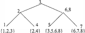
If the pairs of sets do not have a common intersection, we can define a more complex hierarchical notion of separability as follows. Given a family Xr, ... , Xn of sets of variables, a tree representation of the family is a tree T that contains one leaf for each X;. For a variable X E U;Xi, the location of X in T is the lowest node of T such that all subsets containing X are at or

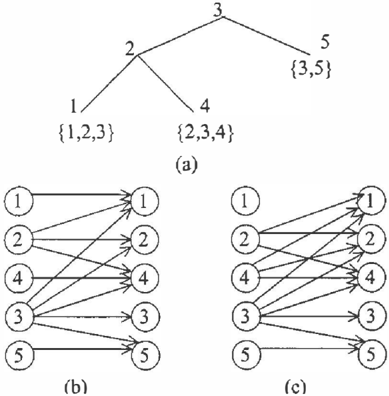
beneath that node. Figure 2 shows an example tree, with each variable shown at its location.

f6.7.8}

Figure 2: A tree representation

For a given tree representation T, let T 1 1 · · . , T m de note the subtrees of T. Let W denote the vari ables at the root of T, and U i denote the variables in the subtree T;. We say that P(Z I u1X;) is T separable if either T is a leaf, or for every assign ment w tow, pw(z I u1 ,···,Um) can be written as 'L,(riPt(Z I U;), where "£;"Yi = 1, and P;.w is T;-separable. Using induction, one can show that x�, .. . ' Xn are sufficient for z iff P(Z I UiXi) is T separable for any tree representation T of X1, ... , Xn.

4 Separability in Temporal Models

4.1 Self-Sufficiency

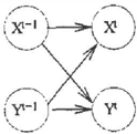
How is all this relevant for temporal probabilistic mod els? Let us look at some examples. First, suppose that there are two state variables xt and yt. Suppose that in the dynamic model specifying P ( X t I xt -l y t - 1) and P(Yt I xt-1 yt-1 ) , xt- 1 and yt-1 are sufficient for xt and also for yt. The DBN structure is shown in Figure 3. In this dynamic model, the state vari ables at any point in time are not independent of each other. Nevertheless, because of sufficiency, if we want to know the marginal distributions over xt and yt we only need the marginals over xt-l and yt-1. And similarly, the marginals over xt and yt will give us the marginals over xt+t and yt+l, assuming their are no observations to condition the distribution at time t. We can therefore propagate marginals to obtain correct predictions of the marginal probabilities of the state variables at any future time point.

Figure 3: A simple DBN

Now, let us increase the number of state variables to n, but still assume that the individual vari ables xi-1, . .. , x�-1 are sufficient for each of the Xf, .. . , X�. The same situation holds - we only need to propagate marginal distributions over each of the Xf to obtain correct predictions of marginals. This is a natural model for a system with a simple information flow, in which at each point in time each variable only receives information from one previous variable, but we don't know which one. We can introduce a matrix "(, where 'Yij is the probability that the variable that influences Xf is xr1. I.e., "Yi is the probability distri bution over which variable influences X; at a point in time. Then, associated with each ij, there is a model P;j (Xf I x;-1) of the particular way in which X; is influenced by Xj.

This type of model is fairly natural for weather sys tems. The state consists of a variable Xi for each lo cation i in a grid. The variable representing a location may actually be compounded from several variables, such as temperature, pressure and water density. At each point in time, the weather at a location depends stochastically on the weather at one of the neighbor ing locations at the previous time, but we don't know which neighbor. Climate modelers talk about "pack ets of air" m o vi n g about from one location to another. In this model, 'Yi encodes the distribution over wind patterns at i, while Pij encodes how a packet of air tends to change as it moves from j to i.

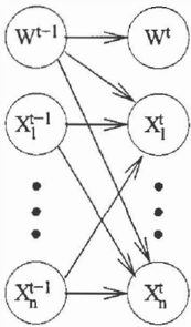
Let us enrich the model. At any point in time, the wind patterns at different points in a region are not independent, but are correlated by the prevailing wind direction. We can model this by introducing another state variable wt indicating the prevailing wind di rection throughout the entire region at time t. This variable will then influence the particular wind pat tern at each location, i.e., for each w there is a 1l". We also make wt depend on W1-1. The DBN is shown in Figure 4. (For convenience, to keep all edges in the model go from one time slice to the next, I have made the wind pattern at location i at time t depend on wt-1 instead of wt.) This DBN actually displays little of the structure traditionally sought in DBNs, since each of the Xf variables depends on all of the other variables at the previous time. Nevertheless, the seperability makes this a highly structured model, and the structure can be exploited.

It no longer holds that individual state variables at time t-1 are sufficient for the state variables at timet. However, the doubletons {wt-1, xJ-1} are sufficient for each Xf. This fact alone is not enough to provide a prediction method via propagating marginals, be cause we need to maintain marginals over {Wt, Xf}, and not just the individual variables. In fact, how ever, the sets {wt-t,x;-1} are sufficient for each {Wt, Xf}. We can see this by checking that for a given value w of wt- 1, pw(W1,Xt I xt-1) = P(Wt I w)Pw(Xf I xt-1) = L,11ijP(Wt I w)PiJ(Xf I Xt1),

Figure 4: Weather DBN

and therefore P(Wt l Xf I xt- 1 , wt-1) is conditionally separable given wt- 1 · As a result, we can propagate marginals over the pairs (Wt, Xf), to obtain correct predictions for marginal probabilities over the pairs at any future time.

These examples motivate the definition of a self sufficient family of sets of variables. For simplicity of presentation, I will assume that all state variables in a DBN depend only on variables from the previous time slice. Of course, real DBN models may be richer, including dependencies within a time slice, but this simplified language captures all we need to develop the theory.

Definition 4.1: Consider a DBN with state variables S. A family of subsets X1, ... , Xn of S is self-sufficient if U;X; = S, and for each i, Xi- 1 , . .. , x�-1 are suffi cient for P{X� I gt-1 ). I

Given a self-sufficient family, we can define for each i a function <I>, from the marginals q;-1 over the x�-l to a marginal over X�. Then, given an initial distribution Po over S and a future time T, we can compute the marginals at time T by the following procedure.

Formula not decoded

It is obvious by induction that this procedure com putes the correct marginals at any future time T, since <I>i always computes the correct marginals at the next time point, given correct marginals at the previous time point. If we have a family with n sets, where the maximum number of variables in a set is m, and the maximum number of values of a variable is b, the cost of this procedure is O(Tnbm). In contrast, if the total number of state variables is M, the cost of pre- diction by propagating complete joint distributions is O(TbM).

4.2 Identifying Self-Sufficient Families

Our goal, then, is to identify self-sufficient families of sets of state variables, in which the individual subsets are small. This was possible in the above examples, but in general it may not be easy to find non-trivial self-sufficient families ( the complete set of state vari ables is of course sufficient for itself).

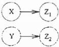
One might think that a technique based on merging variables into compound variables would work, as it did in the weather example. Such a method might be based on the following rule, which seems p la u si ble : if X and Y are sufficient both for Z1 and Z2, and Z1 and Z2 are conditionally independent given XUY, then X andy are sufficient for z = z 1 X z2. Unfortunately, this is wrong. Figure 5 shows a simple counterexample. Here, Z1 and Z2 are deterministic copies of X and Y respectively. Obviously X and Y are sufficient for both Z1 and Z2. However they are not sufficient for zl X z2. The joint distribution over zl and z2 depends on the joint distribution over X and Y, not on their marginals.

Figure 5: A simple counterexample

A more complex rule for merging variables does hold. If xl and y 1 are sufficient for zl' and x2 and y 2 are sufficient for Z2, then Xt u X2, Xt U Y 2, Y t u X2 and y 1 u y 2 are sufficient for z = Zt X z2. However' it is not clear how useful this rule is in actually identifying self-sufficient families. Applying it quickly leads to large sets in the family, and normally it will need to be repeatedly applied until there is a set containing all variables, which is useless.

4.3 Hierarchical Decomposition

A better approach would be to define ways in which a complex dynamic system can be hierarchically decom posed into separable subsystems, such that the fam ily of subsystems is self-sufficient. We can extend the notion of tree representation defined in Section 3 to capture a hierarchical system decomposition. Recall that a tree representation of a family of sets is a tree containing a leaf for each set. The location of a vari able is the lowest node in the tree such that all sets containing the variable are at or beneath the node. A complete tree representation is a tree representation

that has the added property that for every variable X, every leaf beneath the location of X contains X. Figure 6(a) shows a complete tree representation. A complete tree representation of a family of subsystems represents a hierarchical decomposition of the system into its subsystems. Variables at the leaves are con tained in a single subsystem. Variables at intermediate nodes are shared between a local group of subsystems. Variables at the root are shared among all subsystems.

Figure 6: (a) A complete tree representation. (b) Top down mode. (c) {2, 3,4} takes over one level up.

Suppose that we have a complete tree representation, and we would like the family of subsystems it repre sents to be self-sufficient. In static BNs, we saw that sufficiency depends on the way information flows from parent to child: X and Y are sufficient for Z if in formation can only flow from one of X or Y to Z at a time, although we don't know which. A similar ef fect happens in dynamic systems. There may be many different modes of operation in a system, where each mode is characterized by the actual flow of informa tion from variables at the previous time to the current state variables. At any point in time, the system will be in a particular mode, but we may not know what that mode is. In order for self-sufficiency to hold, the different possible modes of operation must all satisfy the property that each subsystem depends on the state of only one subsystem at the previous point in time.

One mode that sastifies this property is a top-down mode. In top-down operation, a variable can only be influenced by variables at the same node or its ances tors in the complete tree representation. Figure 6(b) shows a top-down information flow corresponding to the representation of Figure 6(a). Since variables at a node and its ancestors are all contained in the same subsystem, this ensures that each subsystem will only depend on its own state at the previous time. Cor relations between subsystems are induced via shared variables. Variables that are shared between subsys tems cannot be influenced by variables in individual subsystems.

However, there are other possible modes of operation in which shared variables are influenced by lower level variables. The basic rule is that if a higher level vari able X is influenced by variables within a subsystemS, then S takes over and influences all subsystems sharing X. In particular, another subsystem S' sharing X will not depend on its own previous state, but on that of S. Such a mode of operation is called a take-over mode. Taking over can happen at any level of the hierarchy. At one extreme, a catastrophic event in one subsystem can influence all other subsystems. More commonly, a subsystem will take over the level above it in the hier archy, so that it influences the neighboring subsystems. Figure 6(c) shows an example of a take-over mode in which the set { 2 , 3, 4} has taken over the level above it in the hierarchy. As a result, variables 1 and 2 now depend on variable 4, but variable 1 no longer depends on its own previous state. The root of the hierarchy, variable 3, is not taken over, and the operation in the remainder of the hierarchy is top down.

The mode of operation at a particular point in the hierarchy could be determined by variables higher up. For example, the value of variable 3 could determine whether the mode is that of Figure 6(b) or Figure 6(c). Self-sufficiency allows for some quite rich models. On the other hand, some modes of operation are ruled out by self-sufficiency. In particular, a subsystem cannot depend both on its own internal state and on that of another subsystem at the same time. This rules out some traditional notions of weak interaction between subsystems, in which the state of a subsystem is almost completely determined by its own previous state, but may be perturbed by another subsystem. Separability corresponds to a very different kind of decomposition, in which there is a switch determining what influences a subsystem.

4.4 Observations

I have shown how self-sufficient families allow us to obtain exact predictions of marginals by propagating marginals. What about monitoring, where we want to maintain the distribution over the current state at each point in time, taking into account observations obtained at each time point? Unfortunately, observa tions tend to break sufficiency. The problem is that even if we have the correct marginals over a family of subsets of variables, we do not have the joint distri bution over all the variables. If an observed variable appears in one subset but not others, it should still

condition variables in the other subsets if the variables are not independent in the joint distribution. The marginal distributions do not allow us to perform this conditioning. Therefore, the posterior marginals after conditioning on the observed variable will be wrong.

All is not lost. If an observed variable appears in all subsets in a family, then we can correctly condi tio n in each of t h e subsets to obtain correct poste rior marginals. If a system has a small number of observed variables, and we can contrive to place these variables in the roots of the hierarchical decomposi tion while maintaining self-sufficiency, we will be able to perform exact monitoring of marginals by propa gating marginals. Unfortunately I do not expect this situation to obtain all that often.

5 Conclusions and Speculations

In this paper, I have analyzed a desirable inference property - sufficiency - and shown that it is equiv alent to a representational structure - separability. The analysis extends to more complex notions of suffi ciency and the corresponding structure of conditional separability. I have shown how to exploit separabil ity and conditional separability within the context of Bayesian network inference algorithms.

For temporal probabilistic models, I have shown that some dynamic systems can be decomposed into a self sufficient family of subsystems, that allows for exact prediction of marginal probabilities without propagat ing complete joint distributions. This is satisfying, since as far as I know it is the first non-trivial result of its kind. At the same time, the fact that it does not carry over to monitoring is somewhat disappointing.

The results of this investigation were surprising to me. I began with an intuition that some type of hi erarchical decomposition would lead to the ability to propagate marginals exactly. I expected the struc ture to correspond to some sort of traditional notion of weak interaction, based on local independence or near-independence of sets of variables. It turned out that a very different kind of separability structure was needed, corresponding to simple information flow be tween different subsystems. Systems that have little or no independence, where a variable can depend on many other variables, may still exhibit separability, like in the weather model.

As a result, I believe that studying the information flow in dynamic systems may prove fruitful even when the system is not completely separable. Can sepa rability analysis be integrated with the Boyen-Koller analysis for monitoring? Can the type of information flow decomposition leading to separability be com- bined with other notions of weak interaction to provide for near-separability? If so, how can that be exploited for approximate inference?

Separability may be particularly useful in object-based models in which relationships between objects may vary over time. For example, consider a model of a building and the people in it. At any moment, a per son is only in one room, but we may no t know which. Are there languages that facilitate the definition and identification of separable models?

Finally, it would be interesting to see if notions of sep arability can be useful in decision making frameworks like factored Markov Decision Processes. Like DBNs, these have proven resistant to being exploited for ef ficient solution. It seems that more structure than a factored representation is needed to make solving an MDP tractable. Perhaps separability could provide a clue to finding such a structure.

References

[BFGK96] C. Boutilier, N. Friedman, M. Goldszrnidt, and D. Koller. Context-specific indepen dence in Bayesian networks. In UAI, 1996.

[BK98] Boyen and D. Koller. Tractable infer In

X. ence for complex stochastic processes. UAI, 1998.

[BK99] X. Boyen and D. Koller. Exploiting the architecture of dynamic systems. In AAAI, 1999.

[FKP98] N. Friedman, D. Koller, and A. Pfef fer. Structured representation of complex stochastic systems. In AAAI, 1998.

[ HB 9 4 ]

D. Heckerman and J.S. B r ee s e. A new look at causal independence. Technical report, Microsoft Research MSR-TR-94-08, 1994 ..

S.L. ;Lauritzen. Propagation of proba bilities, means and variances in mixed graphical association models. Journal of the American Statistical Association, 420):1098-1108, 1992.