Support and Plausibility Degrees in Generalized Functional Models

Paul-Andre Monney

University of Fribourg, Seminar of Statistics Beauregard 11-13

CH-1700 Fribourg, Switzerland paul-andre.monney@unifr .ch

Abstract

By discussing several examples, the theory of generalized functional models is shown to be very natural for modeling some situations of reasoning under uncertainty. A general­ ized functional model is a pair (f, P) where f is a function describing the interactions between a parameter variable, an observa­ tion variable and a random source, and P is a probability distribution for the random source. Unlike traditional functional mod­ els, generalized functional models do not re­ quire that there is only one value of the pa­ rameter variable that is compatible with an observation and a realization of the random source. As a consequence, the results of the analysis of a generalized functional model are not expressed in terms of probability distri­ butions but rather by support and plausi­ bility functions. The analysis of a general­ ized functional model is very logical and is inspired from ideas already put forward by R.A. Fisher in his theory of fiducial proba­ bility.

1 The Theories of Bayes and Fisher

Jessica is a young woman suspecting that she might be pregnant. To find out about her status she decides to go to the local pharmacy and buys a pregnancy test. The test result indicates that she is not pregnant, but she knows that such tests are not fully trustworthy. The question is then how to evaluate the chance that she is pregnant in spite of the negative test result.

Of course, one possibility is to use the Bayesian the­ ory to analyze the situation. The Bayesian model is as follows. Let 8 denote the variable indicating her true pregnancy status. The set of possible values of B is e = { -1, +1} where -1 means that she is not pregnant and +1 means that she is pregnant. Simi­ larly, Jet � denote the variable indicating a test result. The set of possible values of� is X = { -1, + 1} where

-1 represents a negative test result and + 1 a positive test result. The reliability of the test can be expressed by two numbers, namely the chance p that the test will indicate a negative result when a woman in not pregnant, and the chance p' that the test will indi­ cate a positive result when a woman is pregnant. It is reasonable to assume that both p and p ' are rather high. This information is represented by the condi­ tional probabilities

Suppose that Jessica's prior about her status is given by the probabilities

Then by Bayes theorem the posterior probability that Jessica is not pregnant is

According to the Bayesian theory, this represents Jes­ sica's degree of confidence in the fact that she is not pregnant.

Now assume that the probability of getting a correct negative result is the same as getting a correct positive result, i.e. p = p'. This means that the test reveals the true pregnancy status with probability p. This probability is an indicator of the confidence in the test result. Then by formula (3) the posterior probability that .Jessica is not pregnant is

This is the Bayesian solution to Jessica's pregnancy test problem. However, .Jessica is unable to give the prior probability of her being pregnant because she is not comfortable with the idea of giving a precise number to estimate this chance. As can be seen in for­ mula ( 4), without a prior it is impossible to find the posterior probability of her not being pregnant. The Bayesian theory requires prior probabilities to com­ pute posterior probabilities. But Jessica is still in­ terested in finding a numerical value expressing the chance of her not being pregnant considering the neg­ ative test result. How can we find such a numerical

value? In 1930, R.A. Fisher identified a class of prob­ lems in which it appeared to him that inductive prob­ ability statements could legitimately be made without prior probabilities being used. It turns out that Jes­ sica's problem when p = p ' is one of them. In this example, Fisher's reasoning would go as follows. First define the variable

The distribution of w is independent of B as the fol­ lowing development shows. First we have

But by equation (5) if B = -1 then w = -� and if e = 1 then w = �. Therefore

and similarly P(w = -1) = 1- p. Fisher called such a variable w a pivotal quantity or a pivot. Generally speaking, a pivotal quantity is a function of 8 and � whose distribution is independent of B. The obser­ vation { = -1 Jessica makes doesn't permit her to infer some information on w because both w ::::: + 1 and w = -1 are compatible with the observation (see equation (5)). So after observing�= -1 we still have P(w = 1) = p and P(w = -1) = 1 - p. These probability statements are as valid as before observ­ ing E = -1. The distribution of w can be seen as a feature of the test device: P(w = 1) = p means that the probability of getting a correct test result is p because w = 1 when e and E indicate the same preg­ nancy status. Under the assumption that w = l, the observation E = -1 logically implies that e = -1 since w = 8 · ( . Since the assumption that w = 1 is true with probability p, it follows that this probability can be transfered to its logical consequence 8 = -1, i.e. P(B = -1) = p. In a similar way, it can be derived that P(B = 1) = 1 - p. This argumentation is an instance of Fisher's fiducial theory. The probabilities P(B = 1) = 1p and P(B = -1) = p represent the so­ called fiducial distribution of B. Fisher noticed that the fiducial distribution coincides with the Bayesian pos­ terior if a uniform prior distribution is assumed for the variable B, but Jessica doesn't have any prior ( not even the uniform one) and so the statement P(B = -1) = p cannot be justified by Bayes' theorem.

There are situations where an observation does pro­ vide information about a pivotal quantity w = g(B, �)­ This information is represented by the set f1' of all w E f1 t h at are compatible with the observation. The elements in n -n' are impossible in view of the ob­ servation. This information is taken into account by conditioning the initial distribution of w on the set f1'. This idea of conditioning the distribution of the pivot is also present in Fisher's fiducial theory. In the fiducial theory, using the pivot w = g(B, ( ) and the ob­ servation� = x, every element o E f1' logically implies that 8 = t for some t E 0. If P' denotes the con­ ditional distribution of w given n'' then the fiducial probability oft is given by the probability of all o E f1' that logically imply B = t, i.e.

2 Generalized Functional Models

In this section we consider models where the spirit and the logic of Fisher's fiducial argument can be applied. However, the theory presented here is not the fiducial theory itself. Within the fiducial theory, the reasoning starts with two variables: the parameter variable 8 and the observation variable �-Then one tries to find a pivotal quantity w = g(B, 0 from which the fiducial distribution of e is determined using the observation.

In generalized functional models we start from three variables: the parameter and observation variables B and w plus a third variable w. The variable w is a random variable whose distribution P is known and assumed to be independent of B. This is a major dif­ ference with the fiducial theory because the fiducial theory requires finding a function of 8 and { whose distribution can be determined and proved to be inde­ pendent of B. In the fiducial theory, conditional dis­ tributions form the initial knowledge before the obser­ vations are made. However, in generalized functional models the initial knowledge is not given by such con­ ditional distributions, but rather by the distribution of w assumed to be independent of B, and by a function of the variables e and w to be described below.

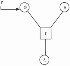
Now generalized functional models are precisely de­ fined. Let !1 denote the set of all possible values of the variable w and as usual l e t 8 and X denote the set of possible values of e and � respectively. It is assumed that there is exactly one correct but unknown value of 8. Let t' be this value. The problem is to generate knowledge about t* in the light of the available infor­ mation. The interaction between the three variables w, � and e is represented by a function

that is determined from the situation under investiga­ tion (see the examples in section 4). The value j(t, o ) specifies what would necessarily be observed if t was the correct parameter value and o was the outcome of the random variable w. It is important to remark that the function f is completely determined from the logic of the situation under investigation. Thus a gen­ eralized functional model is a pair (f, P) where f is a function as in ( 9) and P is a known probability distri­ bution on n that is independent of B.

This figure shows that f describes a relation between the variables w, 8, �and Pis a probability distribution on !!. In a generalized functional model (!, P), sup­ pose that the value of the variable � is observed to be x, i.e. � = x. For the time being, assume that this observation is completely compatible with all possible values of w, i.e.

This means that the observation x could have been generated by any value o E !!. In such a situation it is natural to consider that the distribution P of w remains the same after observing x. The same idea is present in the fiducial theory. Under the assumption that the outcome of the random variable w was a, the observation x logically implies that the correct value of () must be in the set

So the value o is an argument in favor of the hypothesis that t* is in r x ( w ) because if 0 was the outcome then the hypothesis would necessarily be true. Since o was the outcome of w with probability P(o), it follows that o supports the hypothesis that t· E f x(o) to the degree P(o). This reasoning is essentially the same as the one used to define the fiducial distribution of() when an ob­ servation is made. However, in the fiducial theory and in the functional models traditionally considered, the sets r x ( o) are always assumed to be singletons, which is not necessarily the case in this paper (see sections 3 and 4 below). This is why the functional models con­ sidered in this paper are called generalized functional models and not simply functional models. Classical, non-generalized, functional models have been studied by Fraser [3], Bunke [1], Plante [5] and Dawid, Stone [2]. See also Shafer [7].

Now consider the case where the observation x does provide some knowledge about w. This happens when the set

V:c(!!) = { a E!!: 3 t E 8 such that j(t,o) = x } (12) is different from !!. Only the elements of vx ( !! ) are possible values for the outcome of the random vari­ able w in view of the observation x. So the initial probability distribution P of w must be conditioned on Vx (!!). This defines a new probability measure P' on vx ( D ) . Under the assumption that o E vx(!!) was the outcome of w, the observation x implies that t* is in the set

Since o was the outcome of w with probability P'(o), it follows that o in Vx (!!) supports the hypothesis that t· is in fx(o) to the degree P'(o). Remark that fx(o) is not empty for all o E vx(!!).

3 Generalized Functional Models and Hints

The goal of this section is to show how the knowledge about e generated by the observations in a general­ ized functional model can be expressed with the the­ ory of hints, which is a theory strongly related to the Dempster-Shafer theory of evidence [4], [6]. From a generalized functional model (!, P), an observation x generates the set vx (!!) of values of w that are compat­ ible with x. This knowledge is used to condition the probability measure P on vx(D) and let P' denote the resulting probability measure. Using the functional re­ lation f and the observation x, each possible outcome o E Vx (!!) logically implies that t* is in the subset r X ( 0) of e. This defines the mapping

Since o is the outcome of the random variable w with probability P'(o), it follows that o supports the hy­ pothesis that t* E r x(o) to the degree P'(o). Putting things together, the observation x and the generalized functional model (!, P) define the object

which is called a hint. It represents the knowledge about ()generated by the observation x. A hint 'H(x) generates two functions called the support and plausi­ bility functions. The support function is constructed as follows. For an arbitrary subset H � 8, consider the hypothesis that t* is in H. This hypothesis is ei­ ther true or false, but to what extend is it supported by the hint 1-l(x) ? If the outcome of w is in the set

then the hypothesis t* E H is definitely true because if the outcome is an element o in Ux (H) then t* E fx(o) and f,(o) � H, which implies that t* E H. Since the outcome of w is in ux(!!) with probability P'(ux(H)), it is natural to call this probability the degree of support of the hypothesis t* E H (in the rest of the paper, such a hypothesis will simply be denoted by H). The degree of support of the hypothesis H is written sp(H), i.e.

The corresponding function sp: 2 8 -+ [0, 1 ] is called a support function.

It is also interesting to look at the degre of compati­ bility of the hypothesis H with the knowledge about e represented by the hint 'H(x). An element o E v,(O) is compatible with the hypothesis H if it is possible that o is the outcome of w and at the same time H is true. But this is the case when r x(a) n H f. 0. So

is the set of elements that are compatible with the hypothesis H. Since the probability that the outcome of w is compatible with H is P' ( Vx (H)), it is natural to define this probability as the degree of compatibility, or the degree of plausibility, of the the hypothesis H. It is written pl(H), i.e.

This can be done for all subsets H � 9 and the cor­ responding function pl : 26 -+ [0, 1] is called a plausi­ bility function. Elementary properties of support and plausibility functions are listed below:

1. sp(0) = 0, sp(B) = 1
2. pl(0) = 0, pl(B) = 1
3. For all H <; 9, pl(H) = 1 - sp(Hc), sp(H) < pl(H)
4. If H <; H', then sp(H) ::; sp(H') and pl(H) < pl(H')
5. Let H; c e, i = 1, ... , n be a collection of subsets of 9. If we define S = {I � {1, ... , n} : I ::f; 0} then

Property 5 shows that general support functions are not additive measures, e.g. sp(H) + sp(Hc) :S 1. Re­ mark also that the inequality of property 5 would be transformed into an equality if sp was replaced by a probability measure. For simplicity, the abbreviations sp(t) and pl(t) will be used instead of sp({t}) and pl({t}).

Support functions are known as belief functions in the Dempster-Shafer theory of evidence [6]. A function

is a belief function if there exists a function m : 28 -+ [0, 1] satisfying

and such that

for all H c 9. The support function sp associated with the hint H(x) is a belief function whose corre­ sponding m f u n c ti o n is given by

There is a special kind of hints called precise hints. A hint 1{ (X) iS Called preciSe When f x ( 0 ) iS a Singleton for all elements o E vx(fl). For precise hints, the cor­ responding support and plausibility functions coincide and they are probability measures, i.e. sp(H) = pl(H) for all H � e and sp is a probability measure on 8:

for all H <; e. Property (24) holds for precise hints but does not hold in general (see property 5 above).

So far we have considered the case where there is only one observation from which inferences about () is made. Now consider a second observation x' resulting from another realization of the random variable w. We con­ sider it as the outcome of the random variable w' and we assume that w and w ' are independent and iden­ tically distributed random variables before any obser­ vation is made. Let (' denote the observation variable associated with w ' . Of course the set of possible val­ ues of ( and w' are still X and fl and the function f : e X n -+ X is still valid when x' is observed. In the same way as the observation x generated the hint H(x), the observation x' generates the hint

where P" is the conditional probability of P given Vx·(fi). Then the question is: what can be i nfe re d about e given the hints H(x) and H(x') derived from the observations x and x' ?

Under the assumption that the outcome of ( w, w ' ) was (o,o'), the observations x and x' imply that t· E fx(o) and C E fx·(o') and hence t· E rx(o)nfx·(o'). There­ fore, a pair (o,o') such that fx(o) nrx·(o') = 0 is cer­ tainly not the outcome of ( w, w ' ) . So, in view of the observations x and x', the set of possible outcomes of (w,w') is

So the probability measure P' P" must be conditioned on fix,x', which leads to the new probability space (flx,x', Pc,x' ) . The probability Px,x' (a, o') expresses the chance that the outcome o f ( w, w ' ) was (o, o') after observing x and x ' . Putting things together results in the hint

where

for all ( o, o') E flx ,x ' . From this hint degrees of support and plausibility can be computed for any hypothesis H c e we are interested in. This is done in the same wa y as with the hint H(x). For example, the degree of support of H <; 8 is

where

This way to combine two hints into a new hint is called Dempster's rule of combination. As we have seen, this rule is very logical and is an essential element of the theory of hints and belief functions. Two hints having the same support function are called equivalent. If EB denotes the combination operator, i.e.

then it can be proved that EB is commutative and as­ sociative up to equivalence. This allows us to speak of the combination of more than two hints.

When there is a sequence of observations Xt, ... , Xn in a generalized functional model (f, P), the infered knowledge about () is represented by the combined hint

This hint can then be used to determine degrees of support and plausibility of hypotheses of interest in the usual way. Note that the actual computation of such degrees of support and plausibility can be facil­ itated by using special computational procedures in­ volving the so-called commonality functions (for more information on this topic, see [4] or [6]).

4 Examples

4.1 Jessica's Pregnancy Test

Jessica's pregnancy test problem can be analyzed from a functional model perspective. Indeed, from w = () · �, it follows that () · w = �, which defines the function f : e X n � X. Actually, the relations w = () . � and () · w = � are mathematically equivalent, both ex­ pressing the fact that the test device is trustworthy (i.e. w = + 1) when the observed test result (i.e. the value of �) is the same as the actual pregnancy status (i.e. the value of 8). If it is assumed that the test result is a correct indicator with probability 0.9 and a wrong indicator with probability 0.1, then it follows that P(w = +1) = 0.9 and P(w = -1) = 0.1 because w = +1 implies � = e (the test result is a correct in­ dicator) and w = -1 implies � = -e (the test result is a wrong indicator). Remark that in the functional model these two probabilities are part of the initial knowledge about the problem, they are not derived from known conditional probabilities as in the fidu­ cial theory. Since Jessica's test result is negative, i.e � = -1, it follows that V-t ( O ) =nand

which defines the hint

This is a precise hint and therefore the associated sup­ port function is a regular probability distribution given by

So the degree of support that Jessica is pregnant is 0.1 and the degree of support that she is not is 0.9. This is a reasonable result because the reliability of the test device is 0.9 and the test says that Jessica is not pregnant.

In general, if P(w = 1) = p and the test is repeated n times, let k denote the number of positive results and n -k the number of negative results. It can be shown that the hint resulting from the combination of then hints associated with then observations is again a precise hint whose support function is given by

4.2 Policy Identification (I)

In this example, the following real-world situation is considered. Peter is in room A and has a regular coin in front of him. He flips the coin and observes what shows up: either H or T. Then he decides between the following two policies: either tell Paul, who is in room B, what actually showed up on the coin (policy 1) or tell him that the coin showed heads up, regardless of what actually showed up (policy 2). Of course, Paul is unaware of the policy that Peter has chosen. Peter flips the coin n times in total and each time reports to Paul what the chosen policy dictates to tell him. Paul knows that Peter is using the same policy each time the coin is flipped. From the sequence of heads and possibly tails that he receives from Peter, Paul wants to infer information about what policy Peter is using, is it policy 1 or policy 2 ?

To answer this question, Paul builds a generalized functional model of the situation. The parameter space is 0 = { t1, t2} where t1 means, say, that Peter is using policy 1 and t2 that he is using policy 2. The observation space is X = {H, T} (the set of possible reports to Paul after one flip of the coin) and the sam­ ple Space of W is 0 = { Ot, 02} Where 01 means, say, that heads shows up when the coin is flipped and o2 means that tails shows up when the coin is flipped. Since the coin is a regular one, we have P(ol) = P(o2) = 0.5. What is the function f : e X 0 � X in this case ? Let's start with f ( t1, o1). It is clear that under policy 1, if heads shows up then Peter will report H to Paul, which means that f(t1,oi) =H. It can easily be seen that the function f is given by

First let's analyse the situation when only one value is reported to Paul. If H is reported, then the infor­ mation that can be infered on () is represented by the hint

where

It is important to remark that this hint is not a pre­ cise hint because r H ( oi) is not a singleton. Indeed, r H (at) = 0 because if H is reported and the coin shows heads up then Peter could have used either pol­ icy 1 or policy 2. On the other hand, r H ( 02 ) = { tz} because if H is reported and the coin shows tails up

then Peter is necessarily using policy 2. The hypoth­ esis that Peter is using policy 2 is supported with strength P(o2) = 0.5 by the observation H, whereas there is not support in favor of the fact that Peter is using policy 1. So the support function associated with 1i(H) is given by

Since 7-l(H) is not precise, this support function is not a regular probability measure on 8: spH(ti) + S P H (t2) < 1. The plausibility function associated with H(H) is given by

This means that the degree of compatibility of the hy­ pothesis that Peter is using policy 1 with the observa­ tion H is 0.5, whereas nothing is speaking against the hypothesis that he is using policy 2, it is fully compat­ ible with the observation H.

If Tis reported, then vr(D) = {o2} because o1 is ex­ cluded since it is impossible to observe T if the coin turned heads up. This implies that we have to con­ dition P on { 02}, which results in the deterministic probability measure P'(o2) = 1. Since rr(o2) = {ti}, which means that if Tis reported and the coin turned tails then Peter is using policy 1, it follows that the hint derived from the observation T is

Then the corresponding support function is

which means that Peter is definitely using policy 1. The hint 1i(T) is called a deterministic hint on t1 be­ cause it is certain that h is the correct value of the parameter variable e.

Now let's analyze the situation where n reports are made. Let k denote the number of heads reports and nk the number of tails reports (the order in which the heads and tails are reported is irrelevant). The hint on e that can be derived from this collection of observations is

If at least one tails is reported (i.e. nk > 0), then it can easily be proved that H(n, k) is again a determin­ istic hint on t1, which means that Peter is using policy 1. This is reasonable because if at least one tails is reported then Peter can't be using policy 2. If no tails is reported, then it can be proved that 7-l(n, n) is not precise and its support function is given by

Note that sp(ti) + s p (t 2 ) < 1 because 1-i(n, n) is not precise. The corresponding plausibility function is

So the hypothesis t1 is becoming less and less plausible as the number of heads reported increases, which is of course very reasonable.

4.3 Policy Identification (II}

In this example we consider the following real-world situation. Peter is in room A and has two coins in front of him, one red and one blue. Peter tells Paul, who is in room B, that when the red coin is flipped, the probability that heads shows up is p1 and when the blue coin is flipped, the probability that heads shows up is pz. Peter successively flips the red and blue coins and observes what shows up : either H or T for each coin. Then he decides between the following two poli­ cies: either tell Paul what showed up on the red coin (policy 1) or tell him what showed up on the blue coin (policy 2). After the policy is chosen, he informs Paul about what showed up on the coin specified by the policy. Of course, Paul is unaware of the policy that Peter is using. This experiment is repeated n times in total, thereby assuming that the policy Peter is using remains the same throughout all experiments. From the sequence of heads and tails that he receives from Peter, Paul wants to infer information about which policy Peter is using, policy 1 or policy 2 ?

To answer this question, Paul builds a generalized functional model of the situation. The parameter space is 0 = { t1, tz} where t1 means, say, that Peter is using policy 1 and t2 that he is using policy 2. The observation space is X= {H, T}. The sample space is constructed from the two random variables involved in the experiment, namely the result of flipping the red coin (random variable w ) and the result of flipping the blue coin (random variable w'). The sample space of w is 0 = {OJ 1 02} where OJ means that the red coin ShOWS heads up and o2 that it shows tails up. By analogy, we define the sample space 0' = { o�, o2} of the random variable w'. The sample space of (w, w') is then 0 X 0' and the corresponding probabilities are

What is the function f : e X 0 X 0' --+ X in this case ? Let's start with f ( t1, 01, oD. It is clear that under policy 1, if the red coin shows heads up then Peter will report H to Paul, which implies that j(t1, o1, o�) = H and f(ti,oi,o2) =H. It can easily be seen that the complete function f is given by

If H is reported, then

and the conditional distribution of P on vH(O x 0') is the probability P' given by

Also, we have

which shows that the hint

is not a precise hint. Its corresponding support func­ tion is given by

On the other hand, if T is reported, then

and the conditional distribution of P on v r(O x 0') is the probability P' given by

Also, we have

which shows that the hint

is again not a precise hint. Its corresponding support function is given by

Now let's analyse the situation where n reports are made, k of which beeing H and n -k being T (here again the order in which the heads and tails are re­ ported is irrelevant). Then the hint on () induced by the collection of observations is

It can be proved that this hint is not precise and its associated support function is given by

where

5 Prior Information in Functional Models

In a situation where the initial knowledge contains a prior probability distribution P0 on B, it is easy to include this information into a generalized functional model (f, P). Indeed, this prior information can be viewed as a precise hint on () given by

where f(t) = {t} for all () E e. The support and plausibility functions of this hint is nothing but the prior probability distribution P0. Then this hint 1-1.0 is combined with the hint 'H(x1, .. . , x n ) by Dempster's rule of combination to obtain a new hint 1-1. expressing the knowledge about () derived from all the available information about the problem under investigation:

Then, as usual, degrees of support and plausibility can be determined from H. It turns out that 'H is always a precise hint.

On the other hand, from a generalized functional model (f, P) the following conditional distributions of � can be defined:

for all t E e. Such conditional probability distri­ butions specify what is called a distribution model. These conditional distributions together with a prior probability P on () completely specifies a Bayesian model which is denoted by (Pr, P). Then it can be proved that if P0 = P, then the support function as­ sociated with 1-1. (which is a probability measure since 1-1. is precise) coincides with posterior distribution of() given XJ, . . . , Xn in the Bayesian model (Pr, P). In ad­ dition, if 'H (xi, ... , xn ) happens to be precise, then its associated support function coincides with the poste­ rior distribution of() given XI, ... , Xn in the Bayesian model (Pr, pu) where pu is the uniform distribution on e.

Finally, let's mention that it is possible to find two different generalized functional models (h, P1) and (h, P2) having the same associated distribution model Pr(� = xiB = t). This means that generalized func­ tional models have a stronger ability to distinguish be­ tween real-world situations than distribution models, which is an important good quality of generalized func­ tional models.

6 Conclusion

This paper shows that generalized functional models are very natural in some situations of reasoning un­ der uncertainty. The advantage of this type of models is that they are capable of better representing the in­ formation that is really available at the begining of the analysis. For example, there is no need to arti­ ficially create prior information on the variable of in­ terest if originally there is none. But if some is avail­ able, then it can easily be included into a generalized functional model. The analysis of generalized func­ tional models is inspired from ideas already advocated by R.A. Fisher in his theory of fiducial probability. This analysis naturally leads to the use of support and plausibility functions to express the knowledge about the variable of interest that is generated by the avail­ able information. These functions, and not necessarily probability distributions, are the appropriate tools to represent the results of the analysis of a generalized functional model.

References

1. H. Bunke. Statistical inference: fiducial and struc­ tural vs. likelihood. Math. Opemtionsforsch. u. Statist., 6:667-676, 1975.
2. A.P. Dawid and M. Stone. The functional-model basis of fiducial inference. The Annals of Statistics, 10(4):1054-1067, 1982.
3. D.A.S. Fraser. The structure of inference. Wiley, 1968.
4. J. Kohlas and P.A. Manney. A Mathematical The­ ory of Hints. An Approach to the Dempster-Shafer Theory of Evidence, volume 425 of Lecture Notes in Economics and Mathematical Systems. Springer, 1995.
5. A. Plante. On the validation of fiducial techniques. Can. J. Statist., 7:217-226, 1979.
6. G. Shafer. A Mathematical Theory of Evidence. Princeton Univ. Press, 1976.
7. G. Shafer. Belief functions and parametric models. J. R. Statist. Soc. B, 44(3):322-352, 1982.