Testing Implication of Probabilistic De p endencies

S.K.M. Wong

Department of Computer Science University of Regina Regina, Saskatchewan Canada, S4S OA2 wong@cs. uregina.ca

Abstract

Axiomatization has been widely used for test­ ing logical implications. This paper suggests a non-axiomatic method, the chase, to test if a new dependency follows from a given set of probabilistic dependencies. Although the chase computation may require exponential time in some cases, this technique is a pow­ erful tool for establishing nontrivial theoreti­ cal results. More importantly, this approach provides valuable insight into the intriguing connection between relational databases and probabilistic reasoning systems.

pendencies in a manner analogous to proofs in math­ ematical logic. In this paper, we adopt an alterna­ tive method from relational database theory [7, 11] for testing logical implication of probabilistic dependen­ cies. We use tableaux and an operation on tableaux, the chase, to test if a new dependency follows from the initial set of dependencies. Our study will focus on the generalized acyclic join dependency (GAJD) [20, 21]. Probabilistic conditional independencies are a subclass of this dependency.

1 INTRODUCTION

In probability theory, the notion of dependencies (in­ dependencies) play an important role. The knowledge of conditional independencies, in particular, is essen­ tial for developing a viable probabilistic reasoning sys­ tem [9, 12, 13].

Given a set of probabilistic dependencies, there are ad­ ditional dependencies implied by this set in the sense that any joint probability distribution that satisfies the original set must also satisfy the additional de­ pendencies. Developing a qualitative method for test­ ing logical implication of dependencies is important for many reasons. First, it enables us to derive interesting and powerful theorems that may or may not be obvi­ ous from the numerical representation of probabilities. Second, in the design of a probabilistic inference sys­ tem, we often need to know whether one dependency is implied by a given set of dependencies.

Axiomatization has been widely used for determining logical implications [2, 14, 15, 16, 17, 19]. In this ap­ proach, a finite set of complete inference rules are in­ troduced for a particular class of dependencies. These rules are used to generate symbolic proofs for new de-

The chase computation may require exponential time in some cases [11]. However, this approach provides valuable insight into the intriguing connection between relational database and probabilistic reasoning sys­ tems. On the practical side, the chase technique is a powerful tool for establishing some important theoret­ ical results. For example, based on this technique, one can show that a GAJD is equivalent to a set of proba­ bilistic conditional independencies. The chase method can also be used to study the optimization problems in probabilistic reasoning. (The results of these studies will be reported in a separate paper.)

This paper is organized as follows. In Section 2, we first establish the fact that probabilistic knowledge can be represented as a generalized relational database. In particular, we show that a decomposable joint proba­ bility distribution can be conveniently represented as a GAJD. Within this framework, one can view evi­ dential reasoning simply as processing a conjunctive query in a generalized relational database system. In Section 3, we develop the chase algorithm. We show in Section 4 how the chase technique is applied to testing dependency implications. The conclusion is presented in Section 5.

2 GENERALIZED RELATIONAL DATABASE

It has been pointed out that there exists an intrigu­ ing connection between relational database and prob-

abilistic reasoning systems [20, 21]. In this section, we first briefly describe some database concepts pertinent to our discussion. Then we introduce our extended relational data model. We show that a decomposable joint probability distribution is equivalent to a gener­ alized acyclic join dependency (GAJD) in this model, and probabilistic conditional independence is a special case of GAJD. Representation of a GAJD by a tableau will be discussed in Section 3.

2.1 RELATIONAL DATABASE CONCEPTS

Let N be a finite set of variables called attributes. We will use upper case letters A, B, C, . . . to denote a single attribute and . . . , X, Y, Z to represent a subset of attributes. Each attribute A E N takes on values from a domain VA. Consider a subset of attributes X = {A1, A2, ... ,A1} <;;;; N. Let Vx =VA, U VA2 U ... U VA, be the domain of X. AX-tuple tx is a mapping from X to Vx, i.e., tx : X --+ Vx, with the restriction that for each attribute A EX, tx[A] must be in VA. (We write t instead of t x if X is understood.) Thus t is a mapping that associates a value in Vx with each . corresponding attribute in X. IfY is a subset of X and t aX-tuple, then t [Y ] denotes theY-tuple obtained by restricting the mapping toY. Let y = t[Y]. We call y a Y-value which is also referred to as a configuration of Y. A X-relation r (or a relation r over X, or simply a relation r if X is understood) is a finite set of X-tuples or X-values. If r is a X-relation and Y is a subset of X, then by r [Y ] , the projection of relation r onto Y, we mean the set of tuples t [Y ] , where tis in r.

We define a database scheme R = { R1, Rz, ... , RN} to be a set of subsets of N. We call the R;'s re­ lation schemes. If r 1 , r2, ... , r'N are relations, where r; is a relation over R; ( 1 ::; i ::; N), then we call r = { r1, rz, ... , r'N} a database over R. The join (natu­ ral join) of the relations in r (where the join is denoted by either r1 l><l r2 l><l . . . l><l r'N or l><l r ) is the set of all tuples t with attributes R 1 U R2 U .. . U RN, such that t [ R ; ] is in r; for each i ( 1 ::; i ::; N). We say that a relation r with attributes R = R1 U R2 U ... URN obeys the join dependency l><l{ R1 U R2 U ... U RN} = l><lR, if r = l><l {r1,r2, ... ,rN}, where r; = r[R;], for 1::; i ::; N. It follows that the join dependency l><l{ R1 UR2U ... URN} holds for a relation r if and only if r contains each tu­ ple t for which there are tuples t 1 , t2, . . . , t N of r (not necessarily distinct) such that t;[R;] = t[R;] for each i (1::; i::; N).

Multivalued dependency (MVD) [6, 7, 8] is a special case of join dependency (JD) [3, 11]. We say that the MVD X -+-+ Y holds for relation r if for any t1, t2 E r with tl[X] = t2 [X], there exists a tuple t3 E r such that t3[X] = t1[X], t 3 ( Y ] = tl[Y] and t3[R- XY] =

t2[RXY]. By XY, we mean Xu Y.

2.2 AN EXTENDED RELATIONAL DATA MODEL

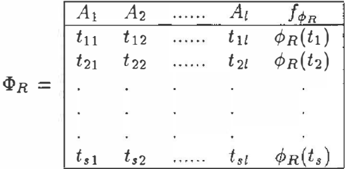
In the proposed relational data model [20, 21], each relation ll> R represents a real-valued function ¢R on a set of attributes R = { A1, A2, ... , Al} as shown in Figure 1, where t;j E VAj, i.e., t; = (t;1,t;2, .. . ,t;t) E VR is a configuration (tuple) of R. The function ¢R(t;), defines the values of the attribute fq,R in relation ll> R· The semantic interpretation of the function ¢ R would depend very much on the particular application.

In the conventional database model, for example, ¢(t) could be interpreted as the number of tuples t in a relation, if one is interested in keeping track of dupli­ cate tuples resulting from a projection. Let ll>u de­ note a universal relation with ¢(t) = 1 for all tuples of U = A1, A2, ... , At. The relation ll>R shown in Fig­ ure 1 can be interpreted as the relation obtained by projecting ll>u onto R = A 1 A2 ... A1 <;;;; U, where ¢ ( t; ) is the number of tuples with t; = t[R] in the origi­ nal relation. Clearly, it is not necessary to use such a function¢ to define a relation, if counting of duplicate tuples is not an issue. We will show that the con­ ventional relational database model is indeed a special case of the extended data model introduced here.

On the other hand, in a probabilistic model, for ex­ ample, the relation ll> R shown in Figure 1 represents a marginal probabilistic distribution. That is, the func­ tion ¢R ( t ) on R, which defines the values of the at­ tribute /q,R in relation ll>R, is a joint distribution (a marginal distribution).

o;l>R =	A1 A2 tll tl2 t21	t22	t11 t21	¢R(t1) ¢R(t2)
	i.t	t,2

We can define an inverse relation (<I>R)1 for <I>R, by setting ¢R(ti)- 1 = rPR(t,), for each t; (1 $ i $ s) with ¢R(t;) :j:. 0. The reason for introducing such an inverse relation will become clear when a specific application is considered.

Apart from the select, project and natural join opera­ tors in a standard relational system, we define here two new relational operators called marginalization and product join.

1. Marginalization

Let X be a subset of attributes of R. The op­ erator of marginalization is denoted by the sym­ bol t. The marginal ¢}:{ of cl> R is a relation on XU {!¢R}. We can construct c�>'k x from cl>R as follows:

• (a) Project the relation ci> R on the set of at­ tributes XU {!¢R}, without eliminating iden­ tical configurations (tuples).
• (b) Lett be a tuple in ci>R[R]. For every configu­ ration t x = t [ X] , replace the set of configu­ rations of XU{! ¢R} in the relation obtained from step (a) by the singleton configuration:

where iR-X = t[ R -X] and t = tx * iR-X· The symbol * denotes concatenation of two tuples.

2. Product Join

Consider two relations ci> x, Wy defined respec­ tively by functions ¢x and 'lj;y. The product join of ci> x and Wy, written ci> x x Wy, is defined as follows:

• (i) Compute the natural join, cl>x N Wy, of re­ lations ci> x and Wy.
• (ii) Add a new column labeled by the attribute !¢x·'</Jy to the relation cl>x N Wy. The val­ ues of the attribute f 4>x ·1/Jy are defined by the product ¢x(t[X]) ·'lj;y(t[Y]), where tis a configuration of XY such that t[X] = tx E cl>x[X] and t[Y] = ty E \lfy[Y].
• (iii) The resultant relation ci> x x Wy is obtained by projecting the relation obtained from step (ii) on the set of attributes XY U {f4>x ·1/Jy }.

Examples illustrating the marginalization and prod­ uct join operators are given in [21]. It should be noted that both the marginalization and product join oper­ ators introduced above can be defined more generally. For example, in step 2(ii), the values of the attribute fq,x 1/Jy can be defined as </>x(t[XJ) o 'lj;y(t[Y]), where o is a b i n ary operator (not necessarily the ordinary multiplication operator). As in this paper we focus on the study of the relationship between relational and probabilistic systems, we have deliberately chosen or­ dinary multiplication to define the product of </>x and 'lj;y. In this context, we have of course in mind the no­ tion of probabilistic conditional independence, and a marginal relation would represent a marginal distribu­ tion. It is understood that in general the choice of the product operator in step 2(ii) and 1(b) of marginaliza­ tion depends on the specific problem being modeled.

It is perhaps worth mentioning at this point that given any relation cl>R, the product join, cl>R x (cl> R )-1, is a unit relation, i.e., ¢R(t) · <Pi/(t) = 1 for all t's in ci> R[R]. In fact, inverse relations become quite useful in the discussion of the probabilistic model.

2.3 GENERALIZED ACYCLIC JOIN DEPENDENCY (GAJD)

First, let us introduce some notions of graph theory pertinent to our discussion. A hypergraph is a pair (N, R ), where N is a finite set of nodes (attributes) and R is a set of edges (hyperedges) which are arbi­ trary subsets of N [4, 18]. If the nodes are understood, we will use R to denote the hypergraph (N, R). An ordinary undirected graph (without self-loops) is, of course, a hypergraph whose every edge is of size two. We say an element R; in a hypergraph R is a twig if there exists another element Rj in R, distinct from R;, such that ( U ( R -{R;} )) n R; = R; n Rjo We call any such Rj a branch for the twig R;. A hypergraph R is a hypertree [10, 1 8 ] if its elements can be ordered, say R1, R2, o .. , RN, so that R; is a twig in {Rt, R2, 0 · · , R;}, for i = 2, . .. , N. We call any such ordering a tree (hy­ pertree ) construction ordering for R. Given a tree con­ struction ordering Rt, R2, ... , RN, we can choose, for i from 2 to N, an integer j ( i) such that 1 ::; j ( i) ::; i1 and Sj(i) is a branch for R; in { Rt, R2, ... , R;}. We call a function j(i) that satisfies this condition a branching for R and Rt,R2,·o·,RN. For exam­ ple, let N = {A1,A2, ... ,A6}· Consider a hyper­ graph R = {Rt={At,A2,A3},RF{At,A2,A4},RF { A2, A3, As}, RF{ As, A6}}. This hypergraph is a hy­ pertree, as there exists a tree construction ordering, R3, Rt, R2, R4. Furthermore, the branching function for this ordering is j(1) = 3, j(2) = 1, j(4) = 3.

Given a tree construction ordering R1, R2, 0 · · , RN for a hypertree R and a branching function j ( i) for this ordering, we can construct the following set of subsets: £ = {Rj(2) n R2, Rj(3) 11 R3, . . . , Rj(N) 11 RN }. It is important to note that this set £ is independent of the tree construction ordering, i.e., £ is the same for any tree construction ordering of a given hypertree. We call £ the mteraction set of the hyperedges in R.

Consider a relation W R over the set of attributes S = R U {fw R } = R1 U R2 U . 0 . URN U {fw R}, where \li R represents a joint probability distribution over the variables R = R1 U R2 U . . . U RN. Suppose the hypergraph R = {R1, R2, ... , RN} is a hypertree. We say that W R satisfies the generalzzed acyclic join de-

pendency (GAJD), written® R [ w R ) , if

which is a sequential monotone join expression. The monotone join operator @ is defined by: for any Ri,Rj � R,

where xis the product join operator and (w1 R ,n R 1) - 1 denotes the inverse relation w 1 R , n R 1· It should be noted that the sequence, R1, R2, . .. , RN, is a hyper­ tree construction ordering of the hypergraph R.

It should be noted that probabilistic conditional inde­ pendence is a special case of GAJD. This can be easily seen as follows. Let R = {Rt, R2}. In this case, the hypergraph R is always a hypertree. Let WR be de­ fined by a probability distribution 1/J R . Clearly, the condition,

can be equivalently expressed as:

namely, R1 and R2 are conditionally independent given Rt n R2.

2.4 REPRESENTATION OF A DECOMPOSABLE PROBABILITY DISTRIBUTION AS A GAJD

By the chain rule of probability, any joint distribution ¢(a1a2 ... a1) can be expressed as:

where a; E VA,, i.e., a; is an A;- value of attribute A; E R = {At, A2, ... , Al}. For convenience, we have written ¢R(at, a2, ... , at) as ¢(a1a2 ... at). The above identity is particularly useful in using conditional in­ dependencies to simplify the representation of a joint distribution. Consider, for example, a distribution on the set of variables {At, A2, As, A4, A5, As}:

The above joint distribution ¢(a1a2asa4a5a6) can then be simplified to:

In fact, this distribution can be depicted by a directed acyclic graph (DAG) which is known as a Bayesian network [14].

For certain applications, it is much more convenient to represent a joint distribution by a chordal (trian­ gulated) undirected graph. A determined undirected graph G depicts the following distribution:

We say that the above distribution is decomposable [14] (relative to the graph G). Note that each maximal clique in G represents a marginal distribution in the numerator of the above equation.

Consider a chordal undirected graph G representing a joint probability distribution ¢R, i.e., ¢R is decom­ posable relative to G. Let R(G) be the hypergraph whose hyperedges are precisely the maximal cliques of G. Thus, R(G) is both chordal and conformal [3, 4), namely, R ( G) is a hypertree. Let £ denote the in­ teraction set of the hyperedges in R ( G) as defined in Section 3.2.

Lemma 1. [9, 14]. If a joint probability distribu­ tion¢ is decomposable relative to a chordal undirected graph G, then ¢ can be written as a product of the marginal distributions of the maximal cliques of G di­ vided by a product of the marginal distributions of the interaction set of R ( G).

It should perhaps be noted that the computation of marginal distributions is a major problem in practi­ cal applications of Bayesian networks as it may eas­ ily become intractable [5]. Fortunately, many efficient algorithms based on the techniques of local propaga­ tion [10, 18] have been developed for computing the marginals of a factorized joint probability distribution.

Note that for convenience, ¢(at,a2,a3, . . . ) is written as ¢(a1a2as ... ) . Suppose the following conditional in­ dependencies hold:

¢(a3ia1a2) = ¢(a3ia1), ¢(a4ia1a2a3) = ¢(a4ia1a2), ¢(asla1a2a3a4) = ¢(asiaza3), ¢(asla1a2a3a4a5) = ¢(a61as).

Suppose a joint distribution ¢R is decomposable rela­ tive to a chordal graph G. Let R = {Rt, R2, .. . , RN} denote the set of hyperedges of the hypertree R( G). Let R = R1 U R2 U . . . U RN. Each hyperedge R; in R ( G ) defines a marginal distribution ¢; of rP R· Let £ = {Rj(2) n R2, R j ( 3 ) n R3, ... , Rj(N) n RN} be the intersection set of R ( G), in which we have tacitly as­ sumed that the sequence R1, R2, . . . , RN is a tree con­ struction ordering for R ( G). The joint probability dis­ tribution ¢R can be represented as a relation if>R over

the set of attributes S = R U {f.pR}, where the values of the attribute f.P R are defined by the function ¢JR. Similarly, each marginal distribution ¢JR, (1 � i � N) is represented by a relation 1l k R ' over S; = R; U {f .p,}, where the values of the attribute f.P R are defined by the function rp R;. '

By Lemma 1 and the definition of product join, the relation 1l R over S can be expressed as:

Since the sequence R1, R2, · . · , RN is a tree construction ordering for R ( G ) , we have for 1 � j ( i) � i 1 and i=2,3, ... , N:

where Rj(i) is a branch of the twig R; in the hyper­ tree. Thus Equation 2 can be written as a sequential monotone join expression as defined in Section 2.3:

This means that the relation 1l R satisfies the G AJD 0R[1lR]-

Theorem 1 A decomposable joint probability distri­ butwn is equivalent to a generahzed acyclic join de­ pendency.

3 MARGINALIZE-PRODUCT-JOIN MAPPINGS, TABLEAUX, AND THE CHASE

As mentioned in the introduction, the main ob j ec­ tive of this paper is to suggest a procedure, called the chase, for testing logical implications of proba­ bilistic dependencies (independencies), the generalized acyclic join dependencies in particular. This method provides an alternative approach to using axiomatiza­ tion [14, 17, 19] for inferring new dependencies from a given set of dependencies.

3.1 MARGINALIZE-PRODUCT-JOIN MAPPINGS

Consider a decomposable joint probability distribution ¢JR on the set of variables R = { At , A2, . .. , Am}, and a hypertree R = { R t , R2, ... , RN} with R = Rt U R2 U ... U RN. The probability distribution cf; R can be represented as a relation 1l R (see Section 2.4) over the set of attributes S = R U {f .PR}, where the values of the attribute fq,R are defined by the function ¢R·

Likewise, each marginal distribution¢; of rp on R;(l � i � N) is represented by a relation 1lk R , overS; = R;U {f.p,}. The marginalize-product-join mapping, written mR(1lR), is a function on relations overS defined by:

i.e., mR(1lR) is a sequential monotone join expression as defined in Section 2.3. Saying that a relation 1lR (r e pr e s e ntin g a probability distribution ¢R) satisfies t h e GAJD, 0R[1lR], is the same as saying mR(1lR) = 1lR.

Very often, we are not interested in all possible rela­ tions on S. We are primarily interested in some subset, say P. As P may be an infinite set, it cannot be de­ scribed by enumeration. Instead, it can be described by a set of constraints ( s u ch as G AJDs). Let C denote a set of constraints, and let P = SATs(C) denote the set of relations that satisfy all the constraints in C. We can now precisely define the notion of logical im­ plication as follows. Let c denote a single constraint. We say that C logically implies c, written C f= c, if SAT(C) � SAT(c). ( Note that we drop the sub­ script S in SATs if no confusion arises.) In subse­ quent sections, we will develop a procedure to test if a given set of constraints C logically implies a GAJD, say ®R[1lR], namely, we want to test if C f= ®R[1lR] holds.

3.2 TABLEAUX AS MAPPINGS

Similar to relational databases [1, 11], this sec­ tion presents a tabular method for representing marginalize-product-join mappings. A tableau is sim­ ilar to a relation 1l R in the extended data model, ex­ cept, in places of values, a tableau is defined by a set of variables. Consider for example, the following tableau T with S = R U {f.p R } ={At, A2, A3, A4} U {f.pR } :

	At A2 A3 A4
at bl	!¢R a3 b2 Pt = rPR(at,bt,a3,b2)
T=	b3 a2 a3 b 4 P2= t/JR(b 3, a2, a3,b4)
a1 b 5	a3 a4 P3 = ¢R(at,b5,a3,a4)

The set S of attributes labels the columns in the tableau; S is referred to as the scheme of the tableau. The p's are the variables of the attribute f oP R . The sub­ scripted a's are called distinguished variables, and the subscripted b's are called nondistinguished variables. Each variable may appear in only one column. Fur­ thermore, only one distinguished variable may appear in each column. By convention, the distinguished vari­ able a; will be the one that appears in the column of

the attribute A;. We assume in this paper that every distinguished variable appears at least once.

Let T be a tableau and let

denote the set of its variables. A valuation J for T is a mapping from V to Vs = VA, x VA2 x ... x VA1 x VA1+1 such that J(v) is in VA, if v is in the column of A;, where S = {A1, A2, ... , A 1, f q,R}, VA,+· = Vf<�R , and VA; is the domain of A;. We extend valuations to apply to rows (tuples) ofT in the obvious manner: if w is the row< Vt,Vz, . . . ,V(+l >in T, then J(w) is the row< J(vt), J(v2), ... , 8(vl+t) >,where J(vi+t) = ¢R(J(w[R])). Applying J to the entire tableau, we have:

We can use tableaux to define mappings between re­ lations over the same scheme. Consider a relation <I> R over S= RU {fq, R } = {At,A2, . . . ,At,!¢ R }. Relation cl>R is defined by a joint probability distribution ¢R on R. Let wd =< a1, a2, ... , at > be the tuple of all distinguished variables. (The tuple w d is not necessar­ ily in T). Let {p1, P2, ... , pk} be the set of variables corresponding to the attribute fq,R. Given <l>R, we can define a relation T( <I> R) over S as follows:

where the values of the function ¢R(J(wd)) may depend on J(pt), J(p2), ... , J(p�;), where J(p;) ¢R(8(w;[R])).

It is always possible to find a tableau T and an ap­ propriate function ¢ for representing a marginalize­ product-join mapping mR defined by:

where R = { R 1 , R2 , ... ,RN} and R = R1 U Rz U . . . U R N = { A1, A2, ... , At}. The relations ct>1 R , are marginals of relation ci> R over S = R U {fr/> R }. Re­ call that <I> R represents a decomposable joint prob­ ability distribution ¢R· This means that the corre­ sponding hypergraph R is a hypertree. In defining the mapping mR, we have tacitly assumed that the se­ quence, R1, R2, ... , RN, is a tree construction order­ ing for the hypertree R, and£ = {RJ(2) n R 2 , RJ(S) n Rs, .. . 'RJ(N) n RN} is its intersection set.

The tableau for mR, TR, is defined as follows. The scheme for TR is S = R U {fq,R }. TR has N rows, w1, w2, ... , WN. Row w; has the distinguished vari­ able a1 in the A;-column exactly when Aj E R;. The

Figure 2: The tableau TR for mR with R {A1A2, A2As, A3A4}.

variable of the attribute f<t> R in row w; is defined by p; = ¢ R ( w ; [ R]). The remaining nondistinguished vari­ ables in w; are unique and they appear in no other rows ofTR.

To complete the definition for the mapping TR, we need to choose suitable values for the function ¢R in the individual rows, < J(al), J(a2), J(a3), J(a4), '!bR(8(wd)) >, such that TR(cl>R) = mR (cl>R ) for any relation <I> R over scheme S. Recall that J (p;) = ¢R(J(w;)). For this purpose, we define 1/!R(J(wd)) as follows:

Note that if o(TR) � cl>R, by substituting the val­ ues ¢R(8(wd[R])) defined by Equation 4 into Equa­ tion 3, it immediately follows that TR satisfies the con­ dition TR(<l>R) = mR(<I>R)· That is, the marginalize­ product-join mapping ffiR and the tableau TR define the same function between relations over scheme S.

Note that the tableau T1, containing only the row w =< wd,¢R(wd) > with ¢R(wd) = ¢>R(wd), is the identity mapping on all relations <I>R over the same scheme .

3.3 THE CHASE

\Ve now describe a computation method, the chase, for testing implication of dependencies (independen­ cies). We will focus primarily on logical implications of GAJDs.

Let P = SA T ( C) be the set of relations <I> R defined by a set C of constraints. We say tableaux T1 and T2 are equivalent on P, written T1 '=P T2, if T1(<I>R ) == T2(<I>R) for all <l> R in P.

We first consider methods for modifying tableaux

while preserving equivalence. A transformation rule for C is a method for changing a tableau T to a tableau T' with T =:p T'. When P is the set of all relations, the set of all possible transformation rules is very lim­ ited. However, when the set of admissible relations is restricted, more rules are available. In this paper, we assume C is a set of GAJDs, and consider only one k i n d of transformation rules, the ]-rules.

A J-ntle corresponding to a GAJD, ® Q [ <I> R ] , is de­ fined as follows: Let the sequence Q1, Q 2, .. . , Qq , be a tree construction ordering for the hypergraph Q = {Q1,Q2, ... , Qq}, and let Cq = {Q1(2l n Q2, Q j(S) n Qs, ... ' Qj(q) n Qq} be its intersection s e t . Consider a tableau T over the scheme S = Ql U Q2U . . . QqU{f,pq} = Q U{f,pq} = RU{fq,R} = { A1, A2, . . . , At, fq, R }. Not e that Q = R. The variable Pi of the attribute !¢R for row w; in T is equal to Pi = q) R ( w ;[ R]). Here we view tableau T as a relation overS. We say that rows Wk1, Wk2, . .. , wk " of T (not necessarily distinct ) are joinable on Q if there exists a row w not in T that agrees with wk; on Qi, i.e . , w[Qi] = wk.[Qi], 1 :5 i :5 q. The variable </> R ( w[R]) in row w is defined by:

Add this row w to T t o form tableau T'.

Equation 5 can be equivalently expressed as:

It should be noted that QJ(i) n Q; = Wj ( i ) n w;, 2 < i :5 q.

Example 2. Consider the tableau TR given in Figure 2. The J-rule for the GAJD, ®{A1A2, A2AsA4}[<l>R ], can be applied to the first row Wt =< a1, a2, b1, b2, ¢R(a1,a2 , b1, b2) > and the second row w2 =< bs, a2, as,b4,¢R(bs,a2,a3,b4) > of TR to generate the row ws =< a1, a2 , as, b1, ¢R(al, a2 , as, b4) > ,where

Figure 3: The result of applying the J-rule for the GAJD, ®{A1A2, A2AsA4}[<I>R), to the tableau TR in Figure 2.

T,' R	A1 Az As A4
	a1 a2 [¢R b, b2 1/JR(al,a2, b1, b2)
	bs a2 as b4 tPR(bs, a2 , as, b4)
	bs b 6 as a4 <P R(bs, b6, as,a4)
	a, a2 a3 b4 ¢R(al, a2, a3, b4)

Tableau T� in Figure 3 is the result of this applica­ tion. Note that we cannot construct the row w = < a1, a2, a3, a4, ¢R(al, a2, as, a4) > since no J-rule exists which applies to attribute A3. 0

Clearly, when the set P of relations over S is defined by a set C of GAJDs, i.e., P = SAT(C), the cor­ responding J-rules can be used to generate for each tableau another tableau. It can be shown that the J-rules associated with a se t C of GAJDs are a Fi­ nite Church-Rosser ( FCR ) system [11]. That is, the resultant tableau r· is unique, independent of the or­ der in which the rules were applied. The tableau T* called the chase of T under C, written chasec (T), is obtained from T by repeated applications of the rules in C until no new row is being generated.

Let To, T1, T2, ... , Tn d e no t e a generating sequence for T in the chase such that To = T, T; is obtained from T; -1 by an application of a rule in c I and Tn = r·. I t is not difficult to see from Equation 6 that T; -1 =:p T;, 1 � i � n. This means that T =:p T*.

4 TESTING IMPLICATION OF DEPENDENCIES

In this section, we demonstrate that the chase is a re­ markable tool for reasoning about dependencies. In particular, we show how it can be used for testing log­ ical implications of probabilistic dependencies ( inde­ pendencies ) . It can also be used to derive nontrivial theoretical results.

We desire a means to test when all the relations <l>R in P described by a set of constraints C ( i.e., P = SAT(C)), satisfy a particular GAJD, say ®R[<I>R] · That is, we want to test if C F= ®R[<l>R] or T R ( <l>R ) = <I> R holds for al l <ll R 's in P. When this holds, the tableau TR for the GAJD, ®R[<I>R], is equivalent to the identity mapping on P. Testing for this condition amounts to showing whether or not TR. = chase c (TR) contains the row< a1, az, ... , at, ¢ R (w d ) > .

Suppose TR . does contain the row w = < wd, ¢R(wd) > , where Wd = < a1,a2 , ... ,at > and

I R I = l. By assumption, R is a hypertree. Let RJ, R2, ... , RN be a hypertree construction ordering for R, i.e., R; is a twig of {RJ, Rz, ... , R;}, 2 :S i :S N. Since the chase procedure is a FCR system, we may assume that the row w was obtained by applying n :S N- 1 distinct }-rules, JJ, h, . . . , Jn, in C sequentially according to the ordering, RN, RN-1, ... , RJ. For convenience, we label the rows, WN,WN-J, ... ,WJ, of TR corresponding to this ordering. Assume that rule JJ corresponds to the GAJD, say 0Q[<I>R], where Q = {RN, RN-J, ... , Rq+I, Q9}, I Q I = N -q + l , and R=RNURN-JU ... UR9+1UQ9. Applying ruleh to the rows, WN,WN-J, ... ,wq+J,Wq ofTR, we obtain from Equation 5 the row w� = < w'[R], ¢ R(w'[R]) >, where

and

Next, we apply rule }z for the GAJD, say Q?JS[<l>R], to the rows, w�, Wq-J, . .. , w,, where IS I= q -s+ 1, and so on. Finally we obtain:

where WN, WN-J, ... , WJ are the original rows of TR corresponding to the relational schemes RN, RN -J, ... , RJ, respectively. Since, by the con­ struction of TR, w;[R;] contains the distinguished ak in the Ak-column exactly when Ak E R;, we have w;[R;] = wd[R;], 1 :S i :S N. Thus, Equation 7 can be written as:

This means that ¢R is a decomposable probability dis­ tribution. Thus, TR. is indeed the identity mapping on P. Since TR =:p Ti, the condition TR ( <I> R) = <I> R is satisfied by all the relations <I> R in P. Similarly, we can show that the converse is true. That is, if C im­ plies the G A J D , ®R[<I>R], TR. must contain the row w = < a1,a2, . . . ,a,,¢R(wd) >,where ¢R(wd) is de­ fined by Equation 8.

It is important to note that the test for whether TR_ contains the row< a1, a2, ... , a1, ¢R(w d ) >can simply

Figure 4: The result of applying the J-rule ® { A t AzA J , AJA4} to the third and fourth rows of tableau T.ft in Figure 3.

T il­ R-	A1 Az A3 A4
	OJ a2 bJ f<t>R bz ¢R ( a J, a2 , b J , b 2 )
	bJ az OJ b4 ¢R (b3,az,aJ,b4)
	bs bs OJ a4 tPR(bs, b6, OJ, a 4 )
	OJ a2 a s b4 ¢R(ai, a2, a3, b4)
	OJ az a s a4 ¢R(al, az, OJ, a4)

be done by checking whether there exists the row w in TR . such that w[R] =< OJ, a2, . .. , a1 >.

The above results are summarized in the following the­ orem.

Theorem 2 Let C and {®R[<I>R]} be sets of GAJDs over the scheme S = R U {f¢R}. Let TR be the tableau corresponding to the GAJD, ®R[<l>R], and let TR_ = chasec(TR) be the result of the chase, where R = { R1, Rz, ... , RN} and R = R1 U R2 U .. . U RN. Then C F ®R[ <I> R] iff there exists a row w in Ti, such that w[R] = wd =<OJ, az, ... , a1 >, where I R I= d.

Example 3. Let TR be the tableau correspond­ ing to the G A J D , ®R = ®{A1A2, AzA3, AJA4}, as shown in Figure 2, and let C = {®{A1A2, AzA3A4}, 0{A1A2As,A3A4}} be a set of constraints. (For sim­ plicity, ®R[<I>R] is written as ®R.) As in Exam­ ple 2, we can apply the J-rule for ®{A1A2,A2A3A4} to the first and second rows of TR to produce the row w3 =< al,a2,a3,b4,¢R(a!,a2,aJ,b4) > in Figure 3. Similarly, the }-rule®{ A1A2AJ, A3A4} can be applied to the third and fourth rows of T.ft in Figure 3 to gener­ ate the row W4 =< at,az,aJ,a4,¢ R(a1,a2,a3,a4) >. Tableau TR_ in Figure 4 is the result of this application.

Note that the expression ¢R(aJ, a2, OJ, a 4 ) in Figure 4 can be expressed as:

Since TR_ contains the row w =< a1,a2,a3,a4, ¢R(a1, a2, OJ, a4 ) >, by Theorem 2, one can therefore conclude that

5 CONCLUSION

We have shown in this paper that the chase technique provides an alternative method for testing logical im­ plication of probabilistic dependencies. Although the chase computation may need exponential time in the worst case, our p r e l i m i n ary investigations indicate that this technique is a powerful tool in the study of d e ­ pendencies and o pt i m i z ati o n problems in probabilis­ tic reas on i n g . More importantly, perhaps, the pr e sen t st u dy further demonstrates the close relationship be­ tw een relational and p ro b a bil i stic k n owle d ge systems.

References

1. A . V . Aho, Y. Sagiv and J.D. Ullman, "Efficient optimization of a class of relational expressions," ACM Transactions on Database Systems, vol. 4, n o . 4, pp. 435-454, 1979.
2. [2) C. Beeri, R. Fagin and J.H. Howard, "A complete axiomatization for functional and multivalued de­ pendencies," Proc. ACM SIG MOD Sy mp o si u m on Management of Data, pp. 47-61, 1977.
3. C. Beeri, R. Fagin, D. Maier and M. Yannakakis, "On the desirability of acyclic database schemes ," .Journal of the Association for Computing Ma­ chinery, v o l . 30, no. 3, pp. 479-513, 1983.
4. C. Berge, Graphs and Hypergraphs. North Hol­ land, 1973.
5. G.F. Cooper, "The c o mputa t io n a l c o m ple x it y of pr o ba b i l i st i c inference using Bayesian belief net­ works," Artificial Intelligence, vol. 42, no. 2-3, pp. 393-402, 1990.
6. C. Delobel, " N o rmal i za t i o n and hierarchical de­ pendencies in the relational data model," A CM Transactions on Database Systems, vol. 3, no. 3, pp. 201-222, 1978.
7. R. Fagin, A.O. Mendelzon and J.D. Ullman, "A sim p lifie d universal relation assumption and its properties," ACM Transactions on Database Sys­ tems, vol. 7, no. 3, pp. 343-360, 1982.
8. [ 8] R. Fagin, "Multivalued dependencies and a new normal form for r elat i o n al databases," ACM Transactions on Database Systems, vol. 2, no. 3, pp. 262-278, 1977.
9. P. Hajek, T. Havranek and R. Jirousek, Uncertain Information Processing in Expert Systems. CRC Press, 1992.
10. F.V. Jensen, "Junction trees -a new character­ ization of de co mp o sab l e hy p e rgr ap hs , " Research Report, JUDEX, Aalborg, Denmark, 1988.
11. D. Maier, The Theory of Relational Databases. Computer Science Press, 1983.
12. R.E. Neapolitan, Probabilistic Reasoning in Ex­ pert Systems. John Wiley & sons, Inc., 1990.
13. J. Pearl, "Fusion, pr o pagat i on and structuring in belief n e tw o r ks," Artificial Intelligence, vol. 29, no. 3, pp. 241-288, 1986.
14. J. Pearl, Probabilistic Reasoning in Intelligent Systems. M o r g an Kaufmann, 1988.
15. J. Pearl and A. Paz, "GRAPHOIDS: a graph­ based logic for reasoning about relevance rela­ t i o ns, " Technical Report 850038 (R-53-L), Cog­ nitive Systems Laboratory, UCLA, 1988.
16. Y. Sagiv and F. Walecka, "Subset dependencies and a complete result for a subclass of em b e d ­ ded multivalued dependencies," Journal of ACM, vol. 20, no. 1, pp. 103-117, 1982.
17. M. Studeny, Kybernetika, vol. 25, no. 1-3, pp. 7279, 199 0 .
18. G. Shafer, "An axiomatic study of c om puta ti o n in hypertrees," School of Business W ork i ng Paper Series, (No. 232), University of Kansas, Lawrence, 1991.
19. S.K.M. W on g , Z.W. Wang, "On ax i oma tiz a ti o n of probabilistic conditional independence," Proc. Tenth Conference on Uncertainty in Artificial In­ t el l i g enc e , 591-597, 1994.
20. S.K.M. Wong, Y. Xiang and X. Nie, "Representation of b a ye s i an networks as relational databases," Proc. Fifth International Conference Information Pr o ce ss i ng and Management of Un­ certainty in Knowledge-Based Systems, 159-165, 1994.
21. S.K.M. Wong, C.J. Butz and Y. Xiang, "A method f o r i m p l ementing a p r ob a b ilis t i c model as a relational database," Proc. Eleventh Con­ ference on Uncertainty in Artificial Intelligence, 556-564, 1995.